HAL Id: in2p3-00346202
http://hal.in2p3.fr/in2p3-00346202
Submitted on 11 Dec 2008
HAL is a multi-disciplinary open access
archive for the deposit and dissemination of sci-entific research documents, whether they are pub-lished or not. The documents may come from teaching and research institutions in France or abroad, or from public or private research centers.
L’archive ouverte pluridisciplinaire HAL, est destinée au dépôt et à la diffusion de documents scientifiques de niveau recherche, publiés ou non, émanant des établissements d’enseignement et de recherche français ou étrangers, des laboratoires publics ou privés.
Model Using GATE Monte Carlo Simulations on the
Grid
Joe Aoun, Vincent Breton, L. Desbat, B. Bzeznik, M. Leabadand, J.
Dimastromatteo
To cite this version:
Joe Aoun, Vincent Breton, L. Desbat, B. Bzeznik, M. Leabadand, et al.. Validation of the Small Animal Biospace Gamma Imager Model Using GATE Monte Carlo Simulations on the Grid. Medical imaging on grids: achievements and perspectives, MICCAI-Grid Workshop, Sep 2008, New York, United States. �in2p3-00346202�
MICCAI-Grid Workshop – Olabarriaga, Lingrand and Montagnat (Eds.), Sept. 6, 2008, New York (NY). 75
Validation of the Small Animal Biospace
Gamma Imager Model Using GATE Monte
Carlo Simulations on the Grid
Joe Aoun1, 2, Vincent Breton2, Laurent Desbat1, Bruno Bzeznik3, Mehdi Leabad4 and Julien Dimastromatteo5
1Grenoble Joseph Fourier University, TIMC-IMAG 2Clermont Ferrand Blaise Pascal University, LPC 3Grenoble Joseph Fourier University, CIMENT 4Biospace LAB, Paris 5
Grenoble Joseph Fourier University, INSERM U877
Abstract
Monte Carlo simulations are nowadays widely used in the field of nuclear medicine. They are valuable for accurately reproducing experimental data, but at the expense of a long computing time. An efficient solution for shorter elapsed time was recently proposed: grid computing. The aim of this work is to validate a Monte Carlo simulation of the Biospace small animal γ Imager and to confirm the usefulness of grid computing for such a study. Simulated data obtained by the validated model of the gamma camera will enable to investigate new algorithms such as scatter and attenuation correction, and reconstruction methods. Good matches between measured and simulated data were achieved and a crunching factor as high as 70 was achieved on a
campus grid.
Contents
1 Introduction 75
2 Materials and Methods 76
3 Results and discussions 80
4 Conclusions and perspectives 84
1 Introduction
Preclinical small animal researches have become a major focus in nuclear medicine [1]. New therapeutic and diagnostic studies are first investigated and validated on mice or rats before their application to
patients. In consequence, we can find many dedicated small field of view scanners for SPECT (Single Photon Emission Tomography) [2, 3] and PET (Positron Emission Tomography) [4] which have been designed in the last decade for these purposes. SPECT images have a very poor quality because generally used models do not incorporate all physical interactions such as scattering (30% of photons in SPECT images are scattered). Monte Carlo Simulations (MCS) have greatly contributed to these developments thanks to their accuracy and utility in the field of nuclear medicine. The use of the MCS has limitations in computing time. Different strategies have been suggested to reduce the computing time such as the acceleration techniques [5]. Another solution to speed up MCS is to combine Monte Carlo and non-Monte Carlo modelling [5]. A third option that has recently been explored is the deployment of computing grids, also known as the parallelization of the MCS [6]. The parallelization consists in sub-dividing a long simulation into short ones. Each MCS uses a Random Number Stream (RNS) to produce the physical interactions in question. The distribution of MCS on multiple computing resources requires that the generated streams are independent. In this work, we report the validation of the Biospace dedicated to small field of view SPECT scanner using the GATE MC simulation toolkit on the CIMENT Grid, a grid deployed on the university campuses in Grenoble.
The paper is organized as follows:
Chapter 2 presents the materials and methods used in this study: we introduce CiGri (CIMENT Grid), the GATE MCS toolkit, the gamma camera we studied and the methods we used to deploy the simulations on the grid and to validate the simulated results compared to experimental measurements. Chapter 3 proposes an analysis of the results of simulation as well as an overall view of the grid performances. Chapter 4 presents a conclusion and perspectives.
2 Materials and Methods
2.1 CiGri grid
CiGri (CIMENT Grid) is a lightweight grid which exploits the unused resources of the CIMENT clusters on the university campuses in Grenoble (France) [7]. It manages by using the OAR resource management system [8], the execution of a large set of parametric tasks (typically more than 100K) by submitting individual jobs to each cluster batch scheduler. One of the rules is that CiGri jobs shall not disturb the local users. CiGri jobs are treated as a zero priority jobs. Thus, a CiGri job is executed only if there is an idle cluster resource. Furthermore, if a local user requests a resource on which a CiGri job is running, then the job will be killed and automatically resubmitted later probably on another cluster. This approach is based on the concept of “best-effort” tasks. CiGri software is composed of several independent modules interacting with an SQL database. Each module is in charge of a specific task: scheduling jobs, submitting jobs, cluster synchronizing, monitoring jobs, collecting results, logging errors and killing jobs. The CiGri infrastructure is accessible through a User Interface (UI). The accessibility was simplified by adopting the same services and configurations on all interconnected clusters, that’s why CiGri is called a lightweight grid. In order to launch a job, a JDL file (Job Description Language) and a multi-parameter file are requested. Output files are first collected automatically by CiGri from the different clusters, then gathered in a compressed file and finally put in an output directory on the UI, so that the user can easily retrieve them. Users have the possibility to monitor and to control their set of jobs through a web interface. CiGri middleware is a free software under GPL licence (http://cigri.imag.fr/).
Aoun et al. Validation of the Small Animal Biospace Gamma Imager Model. 77
2.2 Monte Carlo simulation toolkit
GATE (Geant4 Application for Tomographic Emission) [9] is a new Monte Carlo simulation toolkit based on the general-purpose simulation package Geant4. It was developed in order to model treatment and diagnosis examinations such as radiotherapy, SPECT and PET in the field of nuclear medicine. GATE is an open source code which uses approximately 200 C++ classes from Geant4. User does not have to program in C++ thanks to an extended version of Geant4 scripting version. Thus, the user can easily build a simulation (macro) by using a script language. Many researchers have been using GATE for its flexibility and its accurate modelling of different detector designs and very complex geometries. The major drawback of GATE is the computation time especially when simulating realistic configurations such as voxelized emission and attenuation maps. Several solutions were proposed to accelerate some of the GATE simulations: (i) setting thresholds for the production of secondary electrons, x-rays and delta-rays, (ii) limiting the emission angle to a certain range, (iii) replacing the disintegration scheme by a source of monoenergetic gammas, (iv) parametrizing replicas for the collimator hole arrays (SPECT), (v) compressing voxelized phantom, (vi) techniques such as variance reduction, bootstrapping and jackknifing, (vii) splitting the simulation on a cluster, and recently on the grid [10].
Total GATE availability (max) GATE availability (average) Clusters CPUs Clusters CPUs Clusters CPUs
Day 11 886 7 430 7 125
Nights and Weekends 11 866 7 555 7 215
Table 1 Number of clusters and CPUs available to use GATE on CiGri.
Nowadays, the ‘gridified’ version of GATE is adopted by a growing number of users. The success of this method is related to the fact that the user is able to generate a large number of events using voxelized geometries and to obtain results in a reasonable time. To distribute a long sub-divided simulation on multiple processors, one should also sub-divide the associated long RNS into short ones. However, these short RNS have to be independent because any intra or inter-sequence correlation could lead to inaccurate results. The parallelization of the RNS was accomplished by using the sequence splitting method (also known as the random spacing method). The pseudo random numbers generator (PRNG) James Random (period 2144) implemented by default in GATE was replaced by the Mersenne Twister PRNG due to his
huge period (219937) [11]. The work described in this paper was done by using GATE 3.1.1 built upon
Geant4.8.1. Table 1 shows the number of clusters/CPUs on which GATE was installed. The GATE macro contains a unique random number status and an output filename. These two parameters are renamed according to their appropriate value during the distribution process. Output files were analyzed with the ROOT object oriented data analysis framework.
2.3 The γ Imager: system configuration
The γ Imager is a high resolution planar scintigraphic camera which associates a 4 mm thick NaI(Tl) crystal and a PSPMT Hamamatsu R3292 which leads to a circular 100 mm diameter field of view. While most high resolution cameras use a pixilated crystal, the scintillation crystal of the γ Imager has a continuous 120 mm diameter with a 100 mm circular diameter active area. An aluminium protection layer, 0.8 mm thick, is placed in front of the crystal. The 5 Inch diameter PSPMT is equipped with a bialkali photocathode, 11 multiplication dynodes, 1 reflective dynode and a multiwire anode with 28 (X) + 28 (Y) wires. The readout of the 56 anode signals enables to calculate the spatial position (X, Y) and the energy for each event. A removable low-energy high-resolution parallel hole collimator with 35 mm
thickness is used. The flat-to-flat distance of the hexagonal holes is 1.3 mm and the septum thickness in all directions is 0.2 mm. The whole detection head is surrounded with a 15 mm thick lead shielding. The γ Imager consists of two detector heads, only one head was used in this study.
Figure 1 (a) The Biospace small animal camera modelled with GATE, (b) contribution of the scattered
photons in each component of the simulation where the source is placed at 2 cm from the collimator.
2.4 Simulation of the Biospace gamma camera
The geometry of the γ Imager was accurately described in GATE. Figure 1 (a) shows the model of the detector head. The dimensions and the material of each part of the real camera were modelled as realistically as possible. The detector head simulation was thus composed of the lead collimator, a 1.2 mm air gap space, the aluminium protection, the NaI(Tl) crystal and the lead shielding of the whole head. As the plate scintillation crystal is 4 mm thick, about 38% of the 140 keV incident photons pass through the crystal without interacting. Thus, a significant number of photons will not be detected if we do not take into account the back-compartment. A 10 µm thick gold layer is placed behind the crystal, followed by a 0.39 mm Epoxy layer which separates it from the 1 mm light guide made of quartz. Another 0.15 thick Epoxy layer is positioned behind the light guide followed by the PSPMT, modelled as a 2 mm borosilicate glass entrance window and a 110 mm nickel backpart. The back-compartment of the detector was ended by a 15 mm rear lead shielding. Figure 1 (b) illustrates the relative scattering contribution of each layer in the model (source at 2 cm from the collimator), by counting the scattered events in each particular part divided by the total number of scatter events. During the acquisitions, a solution containing
99mTc, a photon emitter at 140 keV was put in a glass capillary of 1.4 mm inner diameter and 1.8 mm
outer diameter and 6 mm length. The capillary was held by a Pyrex Ruler (150 mm x 40 mm x 3 mm). The Ruler and the capillary were also simulated.
2.5 Validation of the small animal camera
The validation of the small animal SPECT camera is based on the comparison of four parameters measured experimentally with the corresponding simulation data ; Energy Spectra, Spatial Resolution (FWHM), Sensitivity and Image of a capillary phantom. The three first parameters represent three basic features of a gamma camera, while the image of an inhomogeneous phantom allows a visual comparison between experimental and simulated data.
Experimental set-up
In this study, 16 planar acquisitions were made altogether. The radioactive background was first measured during 30 minutes without any activity and was subtracted from all the other measurements after
Relative scattering contribution
0% 5% 10% 15% 20%25% 30% 35% 40%45% Ruler Capilla ry Collim ator Al p rotec tion Cryst al Gold laye r Epox y 1 Ligh t gu ide Epo xy 2 PM T w indo w PM T (b) lead shielding Al protection crystal light guide PSPMT (a) Ruler
Aoun et al. Validation of the Small Animal Biospace Gamma Imager Model. 79
normalizing it to the same acquisition duration. Then, 14 acquisitions were performed using a liquid source of 99mTc (140 keV) which was put in a thin capillary (1.4 mm inner diameter and 6 mm long)
which was considered as a point source. Total activity was 70 µCi (2.59 MBq). The capillary was first placed in the air at 2 cm, 7 cm, 10 cm and 16.5 cm from the detector’s surface. Then, the capillary at 16.5 cm was positioned above a cylindrical beaker (10.5 cm inner diameter and 15.6 cm long) which was put on the collimator. The beaker was used three times: empty, filled with 400 ml (46.2 mm height) and filled with 1000 ml (115.5 mm height) of water. All the seven configurations were performed in a first set of measurements with the source at the center of the camera Field Of View (FOV), and a second set was performed with the source 2 cm off-centered. The sixteenth configuration was performed so as to evaluate the image of the capillary phantom. The phantom consisted of four parallel capillaries (1.4 mm inner diameter and 31.5 mm long), with a capillary-to-capillary distance of 5 mm. The capillaries were filled with 99mTc solutions of different activities (from the least (right) to the most (left) radioactive) (cf. Figure
5 (a) and (b)): 81 µCi, 129 µCi, 220 µCi and 611 µCi. The phantom was 15 mm far from the scintillation camera. Events were recorded in an energy window between 40 and 186 keV for a duration of 5 minutes for each acquisition. The size of the projections was 256 x 256 pixels (pixel size ~ 0.39 mm).
GATE simulations
The fifteen configurations mentioned above were accurately reproduced using GATE. Monoenergetic gamma rays (140 keV) were emitted in 4 π steradians. The physical processes involving photon interactions (photoelectric effect, Compton scattering and Rayleigh scattering) were modelled using the low-energy electromagnetic package of GEANT4, while gamma-conversion was disabled. The energy resolution Full Width Half Maximum (FWHMe) of the camera was modelled by the convolution of the output data using a Gaussian distribution with user-defined mean and FWHM as stated by the manufacturer (11.5% FWHMe at 140 keV). The intrinsic spatial resolution FWHMi was also modelled in the same way (2.2 mm FWHMi at 140 keV).
Parallelization of the simulations
Many models of the camera have been tested in order to obtain the most realistic detector. A big simulation of one billion events was generated for each configuration. The simulation was split into 1000 small simulations, 1 million emitted events each, and was then distributed on CiGri. The 1000 small output files were collected from the grid, merged into one file (on a local CPU) and finally analysed using ROOT. Simulating 1 million events takes 10 minutes on a local CPU (Pentium IV, 3.2 GHz, 1 Go RAM) and requires ~ 30 million random numbers. Thus, a global sequence of more than 30 billion PRN was used for each simulation (which is small for the used Mersenne Twister).
Comparison parameters
Experimental and simulated data were compared basing them on the following quantities:
• Energy Spectra. The energy spectra of events recorded in the whole FOV (40-186 keV), was sketched for five configurations: (i) in air: source placed 2 and 10 cm from the collimator, (ii) in water: source placed at 16.5 cm from the collimator above the empty beaker which then is filled with 4.62 cm and 11.55 cm of water.
• Spatial Resolution. The FWHM of the point spread function (PSF) was calculated for the 14 configurations by drawing a 6 pixels thick profile (~ 2.345 mm) through the point source. Events were detected in the photopic window (126-154 keV) to reduce the noise effects.
• Sensitivity. The system sensitivity, defined as the number of detected events divided by the number of emitted events, was evaluated for the 7 configurations where the source is placed in the center of the FOV. Data were acquired in 3 energy windows: (i) photopic window 126-154 keV, (ii) Compton window 92-125 keV and (iii) total Field Of View (FOV) window 40-186 keV. • Image of a capillary phantom. The image of the capillary phantom was acquired in the whole FOV in the energy window 40-186 keV. A 6 pixels thick profile was also drawn through the 4 line sources seen on the image.
3 Results and discussions
3.1 Energy Spectra
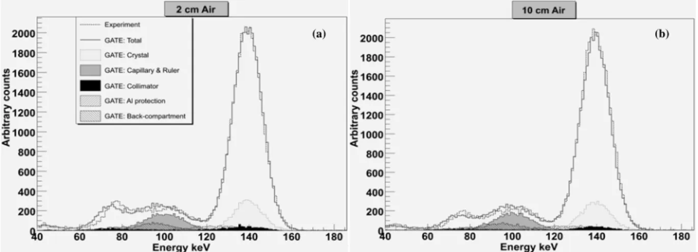
Figure 2 shows the experimental and simulated energy spectra of the 99mTc point source placed in the Air
at 2 and 10 cm from the collimator: contributions of the simulated photons scattered within different components of the detector head and within the capillary and the ruler are also plotted. The experimental and simulated energy spectra were normalized to the same number of counts detected at 140 keV. As illustrated in figure 1 (b), including a back-compartment model was essential as well as the simulation of the capillary and the ruler to obtain a good agreement between measured and simulated spectra between 80 and 120 keV. The contribution of the scattered photons within the capillary and the ruler is clearly higher in figure 2 (a) (source at 2 cm) than in figure 2 (b) (source at 10 cm) especially between 70 and 80 keV. The smaller the ruler-collimator distance, the more the detected back-scattered photons in the ruler.
Figure 2 Experimental and simulated energy spectra for a 99mTc source positioned in Air at (a) 2 cm and
(b) 10 cm from the camera.
Good agreements between experimental and simulated energy spectra can be noticed especially in the photopic and Compton window. Differences could be observed in figure 2 (a) between 60 and 100 keV. These differences are relatively the same between 90 and 100 keV in figure 2 (b) but decrease between 60 and 90 keV where the ruler has the biggest impact. Thus, the difference between 60 and 90 keV could come from the imperfect estimated shape and material of the ruler. For the other difference between 90 and 100 keV, the ruler and the back-compartment have the most important influence according to the figures. It couldn’t derive from the ruler because this difference is relatively the same in figure 2 (a) and (b). Otherwise, the number of scattered photons would increase for the source at 2 cm from the
Aoun et al. Validation of the Small Animal Biospace Gamma Imager Model. 81
collimator. Thus, the difference between 90 and 100 keV could be the consequence of the unawareness of a layer which was not modelled behind the crystal. Energy spectra obtained for the 99mTc point source at
16.5 cm from the collimator, with 0, 4.62 (400 ml) and 11.55 cm (1000 ml) water thickness are shown in figure 3. The scattered photons contributions were also drawn. The scattered photons within the phantom have increased, as expected, proportionally to the water thickness. Good agreements between experimental and simulated energy spectra could be observed for the two configurations with the empty beaker which then is filled with 4.62 cm thick of water. The same differences with the source in Air between 60 and 100 keV were maintained in figures 3 (a) and (b), which confirms that a back-compartment component was not modelled. Significant fluctuations were displayed in figures 3 (b) and (c) because of the low detected events in the corresponding images. This could explain the difference at the top of the photopic in figure 3 (c). The disagreement in figure 3 (c) between 70 and 80 keV and between 110 and 120 keV could be the result of the impurity of the real water used in the measurements.
Figure 3 Experimental and simulated energy spectra for a 99mTc source positioned at 16.5 cm from the
collimator above a beaker filled with (a) 0 cm, (b) 4.62 cm and (c) 11.55 cm of water.
3.2 Spatial Resolution
Centered Source Off-centered Source Distance source-collimator (water thickness) Experimental FWHM (mm) Simulated FWHM (mm) Difference (%) Experimental FWHM (mm) Simulated FWHM (mm) Difference (%) 2 cm 3.34 3.22 3.64 3.58 3.20 10.5 7 cm 4.53 4.54 1.89 4.75 4.53 4.49 10 cm 5.32 5.40 1.47 5.61 5.39 3.95 16.5 cm 7.25 7.34 1.30 7.64 7.37 3.49 16.5 cm (0 cm water) 7.27 7.39 1.63 7.63 7.38 3.32 16.5 cm (4.62 cm water) 7.26 7.32 0.91 7.62 7.26 4.69 16.5 cm (11.55 cm water) 7.58 7.65 0.91 7.83 7.61 2.85
Table 2 Comparison between experimental and simulated spatial resolution for the centered and
off-centered sources placed at: 2, 7, 10 cm and 16.5 in air; 16.5 cm with three water thickness 0, 4.62 and 11.55 cm.
Table 2 shows the experimental and simulated FWHM of the PSF respectively for the centered and off-centered sources positioned in the Air at 2, 7, 10 and 16.5 cm from the collimator. Experimental and simulated FWHM of the PSF for the centered and off-centered sources placed above the phantom (0, 4.62 and 11.55 cm Water thickness) at 16.5 cm from the collimator are also shown. Experimental FWHM for a centered source were well reproduced by the simulations. The disagreements between experimental and simulated FWHM for an off-centered source is lower than 5%, except the source at 2 cm. The 5% differences might be due to the imperfect modelling of the PSPMT non-uniform response in GATE. The approximate modelling of the ruler was also noticed as the disagreements of the FWHM for the source centered and off-centered at 2 cm is clearly higher than the other configurations. An excellent agreement between experiment and simulated FWHM can be observed for the centered sources in water and a disagreement within 5% is obtained for the off-centered sources.
3.3 Sensitivity
The Biospace small animal camera sensitivity values obtained in Air in three energy windows (total FOV 40-186 keV, photopic window 126-154 keV and Compton window 92-125 keV) with GATE compared to the measured values are plotted in Figure 4 (a) for the 4 source-collimator distances 2, 7, 10 and 16.5 cm. Relative differences between experimental and calculated values were respectively: (i) 40-186 keV: 6.8%, 4.6%, 4.1% and 5.7%; (ii) 126-154 keV: 7.9%, 6%, 5.9% and 7.2%; (iii) 92-125 keV: 8.1%, 4%, 1.4% and 5.9%. The results of the system sensitivity with the phantom (empty, 400 ml and 1000 ml) derived from the experiment measurements and the simulations are drawn in figure 4 (b) for the source placed at 16.5 cm from the collimator where events were detected in three energy windows (Total FOV 40-186 keV, photopic window 126-154 keV and Compton window 92-125 keV). Relative differences between experimental and simulated values for the different water thickness (0, 4.62 and 11.55 cm) were: (i) 40-186 keV: 1.5%, 3.8% and 3.1%; (ii) 126-154 keV: 3.2%, 4.4% and 1.9%; (iii) 92-125 keV: 0.3%, 0.5% and 5.6%. The simulation was unable to reproduce the system sensitivity very accurately for the seven configurations described above. This difference could result from the inhomogeneous materials of the different components of the detector which only the constructor accurately knows.
Figure 4 Comparison between experimental and simulated system sensitivities in three energy windows
for the centered source placed at: 2, 7, 10 cm and 16.5 in air; 16.5 cm with three water thickness 0, 4.62 and 11.55 cm.
3.4 Image of a capillary phantom
Figure 5 shows a visual comparison between experimental (a) and the simulated (b) images of the capillary phantom as well as the horizontally drawn profiles (6 pixels thick ~ 2.345 mm) through these images (figure 5 (c)). The comparison of the two images and profiles shows a good agreement. However,
Source in Water 0,0E+00 1,0E-05 2,0E-05 3,0E-05 4,0E-05 5,0E-05 6,0E-05 0 4,62 11,55
Water thickness in the beaker (cm)
Se ns itivity (c ps /B q)
Experiment 40-186 keV GATE 40-186 keV Experiment 126-154 keV GATE 126-154 keV Experiment 92-125 keV GATE 92-125 keV
Source in Air 0,0E+00 1,0E-05 2,0E-05 3,0E-05 4,0E-05 5,0E-05 6,0E-05 7,0E-05 2 7 10 16,5
Distance from collimator (cm)
Se ns itivity (c ps /B q)
Experiment 40-186 keV GATE 40-186 keV Experiment 126-154 keV GATE 126-154 keV Experiment 92-125 keV GATE 92-125 keV
Aoun et al. Validation of the Small Animal Biospace Gamma Imager Model. 83
the simulation was unable to perfectly reproduce the local distortion which could account for the 5% differences between the experimental and the simulated FWHM for an off-centered source.
Figure 5 Comparison between experimental (a) and simulated (b) image of a four capillaries phantom
filled with different 99mTc concentrations and horizontal profiles through the middle of these images (c).
3.5 Calculation time
Table 3 contains the computation time of a long simulation (1000 jobs) on a local CPU (Pentium IV, 3.2 GHz, 1 Go RAM) and on CiGri: during the day, during nights and weekends and an estimated average of the CPUs availability. CiGri has reduced the duration of a simulation compared to 1 CPU computation by a factor of respectively 42, 67 and 56. Resubmitted jobs rate on CiGri, defined as the number of resubmitted jobs divided by the number of executed jobs, is also represented in the box at the right of table 3. 16.9% of the jobs were killed and then were resubmitted by CiGri during the day which is as expected higher than the 10.2% resubmission rate during the nights and weekends. The estimated average of the resubmitted jobs is 13.4%. Each long simulation corresponds to one configuration. The material composition and the thickness of many components of the detector weren't exactly known (PSPMT, Gold layer…). In consequence, about 200 simulations were carried out in order to optimise the model of the Biospace camera. All these simulations would have taken 4 years of computation time on a local CPU, but on CiGri it took only 25 days (table 3). In the ideal case, where no job is killed, the 200 simulations would have taken about 22 days on CiGri. Thus, the 200 simulations would not have been feasible on a local CPU. Reducing the number of simulations would have altered the quality of the results. So the deployment of the Grid was crucial in this study to get accurate results.
1 simulation (1000 jobs) 200 simulations Gain Resubmission percentage (%) Local CPU 167 h 1392 days (~ 4 years) 1 0 CiGri – day 4 h 37 days 42 16.9 CiGri – nights and weekends 2.5 h 21 days 67 10.2 CiGri – estimated average 3 h 25 days 56 13.4
Table 3 Comparison between computing time of 1 and 200 simulations on a local CPU and on the CiGri
Grid with the percentage of the resubmitted jobs (in the box at the right).
4 Conclusions and perspectives
Nuclear medical imaging needs a better physical model to improve the quality of the reconstructed images. Our study has brought into light that the Monte Carlo simulations toolkit GATE was able to accurately model the Biospace small field of view γ Imager. The camera model can thus be used for future researches such as developing new attenuation and diffusion correction algorithms. This paper has also proved the interest of grids in order to obtain accurate results within reasonable elapsed time. CIMENT GRID was an essential tool to carry this study to a successful conclusion. One of our coming studies will be the development of an iterative reconstruction algorithm in which long GATE simulations should be carried out at each iteration. For such studies, a higher scale of computation power is needed. The EGEE (Enabling Grid for E-sciencE) [12] Grid with a next multi-core processor generation should be able to meet our requests.
References
[1] A. Del Guerra and N. Belcari. State-of-the-art of PET, SPECT and CT for small animal imaging. Nucl. Instr. and Meth., A 583 pp 119-124, 2007.
[2] D. Lazaro et al. Validation of the GATE Monte Carlo simulation platform for modelling a CsI(Tl)
scintillation camera dedicated to small-animal imaging. Phys. Med. Biol., 49 pp 271-285, 2004.
[3] F. J. Beekman and B. Vastenhouw. Design and simulation of a high-resolution stationary SPECT
system for small animals. Phys. Med. Biol., 49 pp 4579-4592, 2004.
[4] C. Merheb et al. Full modelling of the MOSAIC animal PET system based on the GATE Monte Carlo
simulation code. Phys. Med. Biol., 52 pp 563-576, 2007.
[5] I. Buvat and D. Lazaro. Monte Carlo simulations in emission tomography and GATE: An overview. Nucl. Instr. and Meth., A 569 pp 323-329, 2006.
[6] V. Breton, R. Medina and J. Montagnat. DataGrid, Prototype of a Biomedical Grid. Meth. Inf. Med., 42(2) pp 143-147, 2003.
[7] Ciment and CiGri project: https://ciment.imag.fr/cigri
[8] OAR: http://oar.imag.fr/
[9] S. Jan et al. GATE: a simulation toolkit for PET and SPECT. Phys. Med. Biol., 49 pp 4543-4561, 2004.
[10] L. Maigne et al. Parallelization of Monte Carlo simulations and submission to a grid environment. Parallel Process. Lett., 2004.
[11] R. Reuillon, D. R. C. Hill, Z. El Bitar and V. Breton. Rigorous Distribution of Stochastic Simulations
Using the DistMe Toolkit. IEEE Trans. Nucl. Sci., 55(1) pp 595-603, 2008.