HAL Id: hal-01445239
https://hal.archives-ouvertes.fr/hal-01445239
Submitted on 24 Jan 2017
HAL is a multi-disciplinary open access
archive for the deposit and dissemination of
sci-entific research documents, whether they are
pub-lished or not. The documents may come from
teaching and research institutions in France or
abroad, or from public or private research centers.
L’archive ouverte pluridisciplinaire HAL, est
destinée au dépôt et à la diffusion de documents
scientifiques de niveau recherche, publiés ou non,
émanant des établissements d’enseignement et de
recherche français ou étrangers, des laboratoires
publics ou privés.
Recommendation for product configuration: an
experimental evaluation
Hélène Fargier, Pierre-François Gimenez, Jérôme Mengin
To cite this version:
Hélène Fargier, Pierre-François Gimenez, Jérôme Mengin. Recommendation for product configuration:
an experimental evaluation. 18th International Configuration Workshop (CWS 2016) within CP 2016 :
22nd International Conference on Principles and Practice of Constraint Programming, Sep 2016,
Toulouse, France. pp. 9-16. �hal-01445239�
O
pen
A
rchive
T
OULOUSE
A
rchive
O
uverte (
OATAO
)
OATAO is an open access repository that collects the work of Toulouse researchers and
makes it freely available over the web where possible.
This is an author-deposited version published in :
http://oatao.univ-toulouse.fr/
Eprints ID : 17217
The contribution was presented at CWS 2016 :
http://cp2016.a4cp.org/program/workshops/ws-config.html
To cite this version :
Fargier, Hélène and Gimenez, Pierre-François and Mengin,
Jérôme Recommendation for product configuration: an experimental evaluation.
(2016) In: 18 th International Configuration Workshop Proce18th International
Configuration Workshop ( CWS 2016) within CP 2016 : 22nd International
Conference on Principles and Practice of Constraint Programming, 5 September
2016 - 6 September 2016 (Toulouse, France).
Any correspondence concerning this service should be sent to the repository
administrator:
[email protected]
Recommendation for product configuration: an
experimental evaluation
Hélène Fargier
1and Pierre-François Gimenez
2and Jérôme Mengin
3Abstract. The present work deals with the the recommendation of values in interactive configuration, with no prior knowledge about the user, but given a list of products previously configured and bought by other users ("sale histories"). The basic idea is to recommend, for a given variable at a given step of the configuration process, a value that has been chosen by other users in a similar context, where the context is defined by the variables that have already been decided, and the values that the current user has chosen for these variables. From this point, two directions have been explored. The first one is to select a set of similar configurations in the sale history (typically, the k closest ones, using a distance measure) and to compute the best recommendation from this set - this is the line proposed by [9]. The second one, that we propose here, is to learn a Bayesian network from the entire sample as model of the users’ preferences, and to use it to recommend a pertinent value.
1
Introduction
In on-line sale contexts, one of the main limiting factors is the diffi-culty for the user to find product(s) that satisfy her preferences, and in an orthogonal way, the difficulty for the supplier to guide potential customers. This difficulty increases with the size of the e-catalog, which is typically large when the considered products are config-urable. Such products are indeed defined by a finite set of compo-nents, options, or more generally by a set of variables (or "features"), the values of which have to be chosen by the user. The search space is thus highly combinatorial. It is generally explored following a step-by-step configuration session: at each step, the user freely selects a variable that has not been assigned yet, and chooses a value. Our is-sue is to provide such problems with a recommendation facility, by recommending, among the allowed values for the current variable, one which is most likely to suit the user.
The problem of providing the user with an item that fulfills her preferences has been widely studied, leading to the content-based and the collaborative filtering approaches, and every variation in be-tween [1, 22, 17]. However, these solutions can’t deal with config-urable products, e.g. cars, computers, kitchens, etc. The first reason is that the number of possible products is huge – exponential in the number of configuration variables. For instance, in the car configu-ration problem described in [4] the definition of "Traffic" delivery vans involves about 150 variables, and an e-catalog of 1027feasible
versions. The second reason is that the recommendation task consid-ered in interactive configuration problem is quite different from the one addressed in classical product recommendation: the system is
1IRIT, CNRS, University of Toulouse, France, email: [email protected] 2IRIT, CNRS, University of Toulouse, France, email: [email protected] 3IRIT, CNRS, University of Toulouse, France, email: [email protected]
not asked to recommend a product (a car) but a value for the variable selected by the user4. Finally, the third reason is that we cannot
as-sume any prior knowledge about the user, nor about its buying habits - complex configurable products, like cars, are not bought so often by one individual. So we have no information about similarity between users (upon which collaborative filtering approaches are based) nor on the preferences of the current user (upon which content-based fil-tering approaches are based).
The present work deals with the the recommendation of values in interactive configuration, with no prior knowledge about the user, but given a list of products previously configured and bought by other users ("sale histories"). The basic idea is to recommend, for a given variable at a given step of the configuration process, a value that has been chosen by other users in a similar context, where the context is defined by the variables that have already been decided, and the values that the current user has chosen for these variables. From this point, two directions can be explored. The first one is to select a set of similar configurations in the sale history (typically, the k closest ones, using a distance measure) and to compute the best recommen-dation from this set - this is the line proposed by [9]. The second one, yet not explored is to learn a from the entire sample a model of the users’ preferences, e.g. a Bayesian net, and to use it to propose a pertinent value.
The paper is structured as follows: the basic notations are pre-sented in Section 2. The next two sections present the two families of approaches that we have explored: Bayesian nets in Section 3 and k-closest neighbors in Section 4. They are experimentally compared and discussed in Section 5.
2
Background and notations
A configuration problem is defined by a set X of n discrete variables, each variable X taking its value in a finite domain X. A complete configuration is thus a tuple o ∈QX∈XX; we denote by X the set
of all of them.
If W is a tuple of variables, W denotes the set of partial configu-rationsQX∈WX; we will often denote such a partial configuration by the corresponding lower case letter w. Also, if W and V are two sets of variables, and if w ∈ w, then w[V ] is the projection of w onto V ∩ W . Furthermore, if w ∈ W , w is said to be compatible with v if w[V ∩ W ] = v[V ∩ W ]; in this case we write w ∼ v. Finally, in the case where w and v are compatible, we denote by w.v the tuple
4Note that we are not concerned here with the choice of the variable – this choice is under the control of the user, not under the one of the recom-mender system. It is worthwhile noticing that the fact that the variables are considered and assigned in a free order forbids the use of techniques based on decision trees.
that extends w with values of v for variables in V \ W (equivalently, wv extends v with values of w for variables in W \ V ).
Not all combinations represent feasible products, because of some possible feasibility or marketing constraints; let P be the subset of X that represent feasible products. In practice, the set P is still a huge set.
In interactive configuration problems, the user builds the product she is interested in through a variable by variable interaction. At each step, let Assigned be the set of variables for which she has already chosen values, u be the tuple values assigned to these variables and UnAssigned the set of free variables ; then the user freely selects the next variable to be assigned (we denoted Next this variable). The system then has to:
• Compute the set of admissible values for Next: it is the set of values v ∈ Next such that there is at least one feasible product o ∈ P with this combination of values, that is o[Next] = v and o[Assigned] = u. The computation of this set has been studied elsewhere [3, 15, 16, 6].
• Propose a recommended value for Next, chosen among the ad-missible values.
The computation of a pertinent recommendation is the topic of the present work.
The recommendation of feature values, when any, is often limited to the proposition of a default value, generally the one advised by the seller in a static way or through a set of rules. Other approaches are based on similarity measures and propose to determine the k-nearest neighbor configuration that are similar to the current set of user re-quirements. These type of approaches support the idea that the user sets her most important requirements and let the system complete the configuration but seldom takes place in a process of interactive configuration (the reader shall consult [13] for a survey about recom-mendation technologies for configurable product).
In the context considered by this paper, sales histories are avail-able, on which the system can rely to base its recommendation. For-mally, a sale history is a (multi) set H ⊆ X of complete configura-tions that correspond to products that have been bought by past users (thus they are feasible, i.e. belong to P ). In the sequel, for a partial configuration u, #(u) will denote the number of configurations in H that extend u.
3
Recommendation with Bayesian networks
Users have different preferences, depending on the taste and the environment of the user, which make them prefer different products -hence a large variety of products in the histories. We do not have any information about their taste, nor do we use any information about their environment. Instead, it can be assumed that there is a ground probability distribution p over the set of complete configurations (i.e. the space of all feasible products), indicating how likely it is that each object is the one that the current user prefers. This probability may depend on her personality, and on her current environment, but it can be assumed that the sales history gives a good approximation of that probability distribution: the configured products eventually bought by the past users are the one they prefer.
Therefore, if Next is the next variable to be assigned a value, and if u is the vector of values that have been chosen for the variables already decided, we propose to estimate, for each possible value v for Next, the marginal conditional probability p(Next = v | Assigned = u): it is the marginal probability that Next has value v in the most preferred product of the current user, given the choices
that she made so far; hence we can recommend the most probable value (among the admissible ones):
argmax
v∈Next
p(Next = v | Assigned = u).
The idea of our work is that the sale history is a sample of X according to the unknown distribution p, that we can use to estimate probabilities. A first, naive method to compute p(v | u) would be to count the proportion of v within the sold products that verify u. Even if this idea works for small u’s, after a few steps the number of products that verify u would be too low and the computations would not be reliable enough (and even impossible when no product in the history verifies u). Hence the idea of learning, off-line, a Bayesian network from the data set and to use it, on-line, during the step-by-step configuration session: the user defines a partial configuration u by assigning some variables and chooses a variable Next ; the recommendation task consists in computing the marginal p(Next | Assigned = u) and recommending the user with the value of Next that maximizes this probability.
3.1
Bayesian networks
A Bayesian network (BN) [21] over set of variables X is defined by a directed acyclic graph (DAG) over a X , and a set of local conditional probability tables (CPT), one for each variable of X . If N denotes a Bayesian network, for X ∈ X we denote by PaN(X) the set of
parents of X in the graph; the local probability table associated to X specifies the probability pN(X = x | u) for every x ∈ X and every
u ∈ PaN(x); if U denotes the parents of X, we denote the table
associated to X by ΘN(X | U ).
A Bayesian network N uniquely defines a probability distribution pN over X : the probability of a complete configuration o ∈ X is
pN(o) = Y X∈X ΘN(o[X] | o[PaN(X)]) = Y X∈X ΘN(X, o).
Example 1. Consider following Bayesian network:
A C E
F D
B
The probability of a configuration abcdef can be computed as: Θ(a)Θ(c | a)Θ(e | c)Θ(f )Θ(d | cf )Θ(b | ad) and Θ(D, abdcf) is defined to be Θ(D | cf).
In the sequel, we will often omit the subscript N when there is no ambiguity.
3.2
Learning a Bayesian network
The learning of Bayesian networks from data proceeds in two steps: finding the structure of the network, i.e. of the DAG underlying the Bayesian network and then its parameters, i.e. the conditional prob-abilities table. Both aim at maximizing likelihood estimates, i.e. the probability of observing the given set.
Since learning the most probable a posteriori Bayesian network from data is an NP-hard problem [7], heuristic strategies had to be found. There are two main families of approaches in structure learn-ing: the score-based ones and the constraint-based ones.
The formers search for a network that maximizes a score pointing out to what extend the network fits the data [8]. The score may be a Bayesian function, such as Bayesian Dirichlet scores (analysed in [12]), or come from information theory, such as the Bayesian Infor-mation Criterion [23] or the Akaike InforInfor-mation Criterion [2].
The latter approach looks for conditional independences, through independence tests, assuming the faithfulness of the network to learn. An early example is the Inductive Causation algorithm of Pearl [27] ; a more recent one is PC [25].
Finally, hybrid method exist, such as MMHC [26], that learns the undirected structure of the network with a constraint-based approach (named MMPC) and then orients the edge of the DAG with a score-based method. Another example is Sparse Candidate (SC) [14].
3.3
Computing marginals
The computation of the posterior marginal probability p(Next | Assigned) is a classical task of Bayesian inference. In gen-eral, it is broken down into computations of two separate prior marginals, since, by definition p(Next | Assigned) = p(Next ∧ Assigned)/p(Assigned).
Recall that, for a given configuration o, p(o) is defined to be the product of local, conditional probabilities that correspond to o in the CPT’s of the network. Then, given a variable X ⊆ X and a partial configuration x ∈ X, the marginal probability p(x) is the sum of the probabilities of the complete configurations that extend x:
p(x) = X w ∈ X w[X] = x = X w ∈ X w[X] = x Y Y ∈ X Θ(w[Y ] | w[P aN(Y )]).
Computing such prior marginals is known to be an NP-hard prob-lem when p is represented by a Bayesian network [10]– the size of the formula can grow exponentially fast with the number of vari-ables. Exact inference algorithms, such as variable elimination [28], value elimination [5], jointree algorithms [19], cutset conditioning [20], recursive conditioning [11], work by breaking down this sum-product formula, into sub-sums and sub-sum-products. These algorithms have a worst-case time complexity exponential with respect to the treewidth of the network. Variable elimination and jointree methods [19] are costly in space while recursive conditioning allows an any-space inference and can be polynomial in any-space. Even if they target a NP-hard task, the algorithms are efficient enough on real world benches to allow an on-line use.
3.4
Recommendation using Naive Bayesian
Networks
In a Naive Bayesian network, one central variable (the one on which inference is to be made) is targeted and the others are assumed in-dependent from each other conditionally to this variable of interest. A naive Bayesian network is therefore a Bayesian network the struc-ture of which is a tree, and where the variable of interest (in our case, Next) is the parent of every other variables (in our case, the vari-ables in Assigned). For any value v of Next and any assignment u of Assigned, we know that P (v|u) is proportional to P (vu); under the strong assumptions of the naive Bayesian network:
P (vu) = P (v) Y
X∈Assigned
P (u[X] | v)
So we will recommend the value v that maximizes
P (v|u) ∝ P (v) Y
X∈Assigned
P (u[X] | v)
Since the variable we are recommending a value for depends on the configuration process, we would need a naive Bayesian network for every variable: to recommend a value for Next, we would use the naive Bayesian network for which Next is the variable of inter-est. The computation of the networks is preprocessed: (all) the prior distributions P (X) and (all) the conditional tables P (Y |X) (i.e., po-tentially all the naive Bayesian networks) are computed off line, be-fore the configuration process, from the sample:
P (X = x) = #(x)
|H| for each X ∈ X
P (Y = y|X = x) = #(x.y) + 1
#(x) + |Y |for each pair X, Y ∈ X The (pre)computation of n prior tables and n2conditional
proba-bility tables are thus sufficient to make a prediction for any variable at any moment.
The strong assumptions of naive Bayesian networks is generally inconsistent: when we want to recommend a value for Next, we as-sume that all the variables in Assigned are conditionally independent given Next. In spite of this naive and strong assumption, they are ef-ficient enough for some applications. Among their qualities, they are easy to learn and easily scalable, requiring a number of parameters quadratic in the number of variables.
4
k
-nearest neighbor
In [9], three algorithms are proposed that are based on the selection of a neighborhood: rather than computing the preference from the entire sample, the system should focus on sold configurations that are similar to the present one - i.e. use the k nearest neighbors. All the methods proposed in [9] are based on the Hamming distance; namely, given an assignment u of Assigned, and a complete configuration w, d(u, w) counts the number of variables in Assigned on which the two configurations disagree:
d(u, w) = | {x ∈ Assigned | u(x] 6= w[x]} |
At each step, these methods first selects the set N(k, u) of the k-nearest neighbors of the current partial configuration u, and compute the recommendation on this basis.
4.1
Weighted Majority Voter
The simplest algorithm is the Weighted Majority Voter, which pre-dicts the value of Next on the basis of a weighted majority vote of the k nearest neighbors. The weight of a configuration w in N(k, u) is set equal to the degree of similarity between this configuration and the current one, u, i.e. the number of variables that are given the same value by both:
weight(u, w) = | {X ∈ Assigned | u[X] = w[X]} | The recommended value for Next is chosen among the ones that are authorized by the constraints by maximizing:
vote(v) = X w ∈ N (k, u) w[Next] = v
4.2
Most Popular Choice
Most Popular Choice predicts the most popular (actually, the most probable) extension of the current configuration, u, from the knowl-edge of the closed neighbors and recommends the value supported by this configuration. It holds that, for any full configuration uw that extends u, P (uw) = P (u|w).P (w). [9] make the assumption that the variables that have not been assigned are mutually independent, and that the ones that are assigned are independent from one another given w. Hence we have:
P (uw) = ΠX∈X \AssignedP (w[X]) . ΠX∈AssignedP (u[X]|w)
The probabilities are estimated from the k nearest neighbors of u: • for X ∈ X \ Assigned and x ∈ X :
P (x) = 1 k|{w
′
∈ N (k, u), w[X] = x}|;
• for X ∈ Assigned and x ∈ X , let N (k, u, w) be the set of neigh-bors of u that agree with w on Assigned: N(k, u, w) = {w′ ∈
N (k, u), w′[Assigned] = w[Assigned]}, then P (x | w) is the fraction of N(k, u, w) that has value x, with a kind of m-estimate correction since N(k, u, w) may be empty:
P (x|w) = |{w
′
∈ N (k, u, w)|w′[X] = x}| + 1 |N (k, u, w)| + k
The value recommended for variable Next is the one prescribed by the w that maximizes P (uw). The drawback of this method is that nothing guarantees that the value computed is compatible with u according to the constraint.
4.3
Naive Bayes Voter
The Naive Bayes Voter is similar to the Naive Bayes method pro-posed in Section 3.4, with the difference that it uses the k nearest neighbors to build a naive Bayes network. Since these neighbors de-pends on the current configuration, is not possible to preprocess the computation of the probability table - this approach may be much slower than the classical naive Bayes.
N ext
X1 X2 . . . Xk
Figure 1. The naive Bayesian network built by Naïve Bayes Voter. Next is the variable of interest.
The recommended value for Next is chosen among the ones that are authorized by the constraints by maximizing P (v|u) ∝ p(v)QX∈Assignedp(u[X] | v), where:
• p(v) =1
k|{w ∈ N (k, u)|w[Next] = v}|
• for every X ∈ Assigned and every v ∈ Next, let N (k, u, v) be the set of neighbors of u that have value v for Next, then
p(u[X] | v) = |{w ∈ N (k, u, v)|w[X] = u[X]}| + 1 |N (k, u, v)| + k
5
Experiments
The approaches proposed in this paper have been tested on a case study of three sales histories provided by Renault, a French automo-bile manufacturer5. These data sets, named “small”, “medium” and
“big”, are genuine sales histories - each of them corresponds to a configurable car, and each example in the set corresponds to a con-figuration of this car which has been sold:
– dataset “small” has 48 variables and 27088 examples. – dataset “medium” has 44 variables and 14786 examples. – dataset “big” has 87 variables and 17724 examples. Most of the variables are binary, but not all of them.
We used the R package bnlearn to learn the Bayesian networks [24] - more precisely, we used Hill Climbing (HC) to learn the two datasets of about 50 variables (small and medium) and MMHC to learn the big dataset of about 90 variables. The average number of parents of a node in the obtained BN is about 1.17, 1.02 and 0.98 - for small, medium and big, respectively. As to Bayesian inference, we used the jointree algorithm provided by the library Jayes [18]. We implemented the Naive Bayes approach and the algorithms based on the k nearest neighbors (k is set to 20 in the experiments reported here; other values of k do not improve the results).
5.1
Experimental protocol
We used a two-folds cross-validation: each dataset has been cut by half, an algorithm learns with one half (which constitute the sale his-tory) and is tested with the other (which can be view as a set of on-line configuration sessions).
The protocol is described in Algorithm 1. Each test is a simu-lation of a configuration session, i.e. a sequence of variable-value assignments. In real life, a genuine variable ordering was used by the user for her configuration session and the different sessions gen-erally obey different variable orderings. Unfortunately, the histories provided by Renault describe sales histories only, i.e. sold products, and not the sequence of configuration in each session. That is why we generate a session session for each product P in the test set by randomly ordering its variable-value assignments. Then, for each variable-value assignment (X, x) in this sequence, the recommender is asked for a recommendation for X, say r: r may be equal to x; or not, if r more probable than x according the inference process ; then X is set to x. We consider a recommendation as correct if the recommended value is the one of X in the product P (i.e. if r = x). Any other value is be considered as incorrect.
The recommendation algorithm is evaluated by (i) the time needed for computing the recommendations and (ii) its success rate, obtained by counting the number of correct and incorrect recommendations.
5.2
Oracle
In order to easily interpret the results of the cross-validation, we pro-pose to compute the highest success rate attainable for the test set. If we where using an algorithm that already knows the testing set, it would use the probability distribution estimated from this testing set. Therefore it would recommend for the variable Next, given the assigned values u, the most probable value of X in the subset of products, in the test set, that respect u. More precisely, for any x in the domain of Next, it would estimate p(x|u) as #(ux)/#(u). Notice that #(u) is never equal to zero, since the test set contains
5 available at http://www.irit.fr/~Helene.Fargier/BR4CP/ benches.html
Algorithm 1: Protocol for evaluating value recommendation in interactive configuration
Input: The training set Htr and the testing set Htest Output: The success rate
main :
1 learning of Htr 2 success← 0 3 error← 0 4 Assigned← ∅ 5 for eachP ∈ Htest do
6 session← randomly order the variable-value assignments
in P
7 Assigned← ∅
8 for each(Next, x) ∈ session do
9 r ← recommended value for Next given Assigned 10 ifr = x then increment success by 1
11 else increment error by 1
12 Assigned← Assigned ∪ {(Next, x)} 13 return success/(success + error )
at least one product consistent with u: the one corresponding to the current session. It is an algorithm overfitted to the testing set.
We call this algorithm “Oracle”. Its success rate is higher than the one of any other strategy. Its success rate isn’t 100% since there is an intrinsic variability in the users (otherwise only one product would be sold . . . ). The success rate of the “Oracle” is generally not attainable by the other algorithms, because the “Oracle” has access to the testing set, what is obviously not the case of the algorithms we evaluate.
5.3
Results
The experiment have been made on a computer with a quad-core processor i5-3570 at 3.4Ghz, using a single core. All algorithms are written in Java, and the Java Virtual Machine used was OpenJDK.
Success rate
Figures 2, 3 and 4 give the success rate of the pure BN-based ap-proach (BN and Naive Bayes) on the one hand, and of the methods based on k closest neighbors on the other hand, on our configuration instances. The experiment is completed with the application of the configuration protocol on classical Bayesian networks benchmarks [24]6. The oracle is given as an ideal line.
It appears that on the configuration instances, the pure naive based approach, which makes very strong independence assumptions, has a low success rate (this error rate is bad also on classical BN bench-marks). This is not surprising, since the variables are not independent from one another, at least because of the constraints. The indepen-dence assumptions at work in the methods based on the k closest neighbors are in a sense less drastic, since the distance used to select the neighborhood implicitly captures some dependencies.
On configuration problems, 3 methods are have very good results: Classical Bayes Net, Naive Bayes Voter and Most Popular Choice. Their success rate is very good (only a few points from the Oracle). The gap with the Oracle gets larger when the number of assigned
6On these benchmarks, the protocol remains the same but has another inter-pretation: the assignment of a variable corresponds to the conditioning of the knowledge base by an observation; the "recommendation" then corre-sponds to the inference of the most probable value for a variable of interest
variables increases: the Oracle’s performance becomes less and less attainable. Indeed, the prediction of the Oracle relies on the testing sample, that includes the product of the ongoing configuration. When few variables are instantiated, the Oracle uses a rather big subsample to make its estimation. When a lot of variables are instantiated, the Oracle uses a small subsample, so small that sometimes it contains only the ongoing configuration. In this case, the Oracle can’t make a bad recommendation. This can be interpreted as overfitting, since the Oracle is tested on the sample it learned. This phenomena is es-pecially visible with the dataset “big”, because it has more variables that “small” or “medium”.
Classical Bayes is the more accurate method on BN instances we tested (hailfinder, alarm, child, insurance, see e.g. Figure 5 for the in-surancebench), which is not surprising either, because the network learnt precisely captures the indepedencies (the sample is perfectly faithful to the BN). But the Naive Bayes Voter and Most Popular Choice do not perform so bad on these instances, from which it can be concluded that these approaches capture a great part of the depen-dencies, even not explicitly.
CPU time
The CPU time (see Figures 2, 3 and 4) clearly breaks the set of algo-rithms in two groups: the ones that learn, off-line, the dependencies from the entire data set and the ones that compute a new neighbor-hood at each step.
The former group of method are one order of magnitude quicker than the latters on the small and medium instances (and some times two: Weighted Majority voter, which has good performances in terms of prediction, is much slower). This is explained by the time needed to extract the k best neighbors before computing the recommenda-tion. On the other hand, this time is not too sensitive to the size of the problem - it remains low on the big instance.
One can check that on this data set, which corresponds to a real world application, the CPU times of all the method tested are com-patible with an on line use, with less than 10 ms in any case. Un-surprisingly, the approximation by a naive Bayesian net is the one that run the fastest (less than 0.05 ms in any case). The time need by Classical Bayesian Nets is in the same order of magnitude, less than 0.1 ms, for the small and medium data set. It stays under 0.25 ms for the big data set.
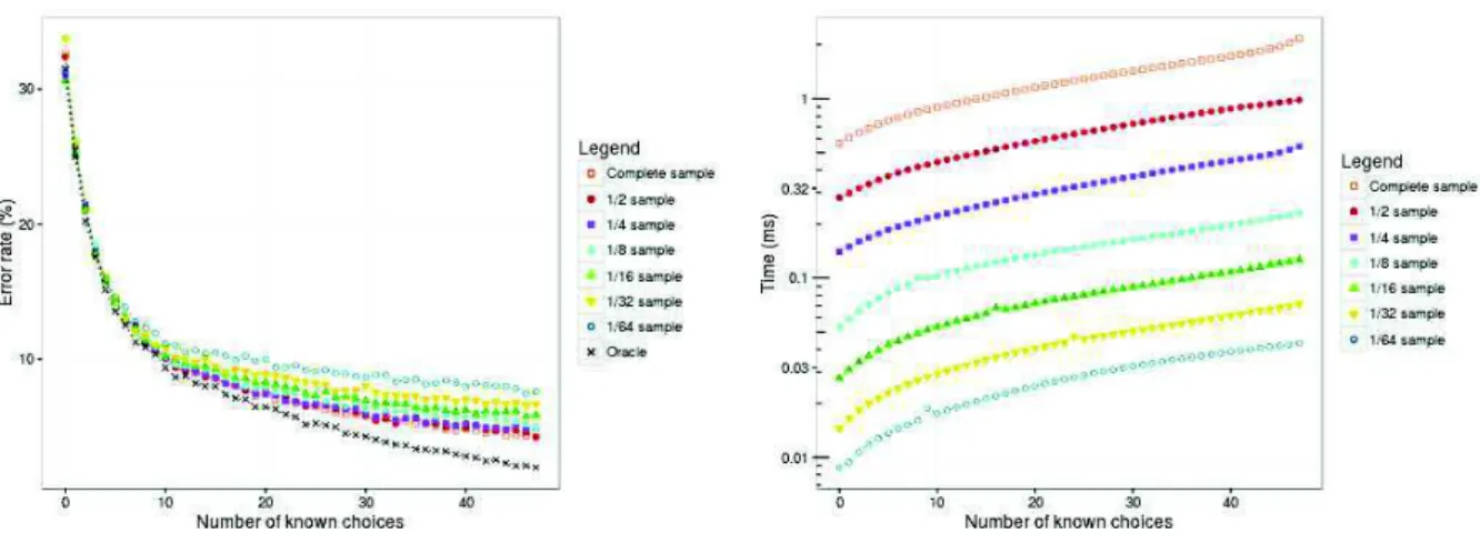
Influence of the sample’s size
The drawback of the methods based on a neighborhood is that their performances seem to depend on the size of the original sample: the greater, the better the prediction but the higher the time needed to make it. To confirm this, we performed another experiment, varying the size of the sample (from the full sample to a sample containing only 1
64 th
of the original one).
This of course leads to an improvement of the performances in terms of CPU and space, but also to a a strong degradation of the accuracy. As a matter of fact, on the small data set, the handling by Most Popular Choice of a sample of 1
32 of the original one needs
twice less time, but the error rate stay over a 9% line (instead of an average of 4%). Naive Bayes Voter and Classical Bayesian Networks are more resistant: for Naive Bayes Voter the time for handling a sample of 1
32 of the original one is divided by 3, with an error rate
Figure 2. Average error rate and time on dataset “small”
Figure 3. Average error rate and time on dataset “medium”
Figure 5. Average error rate and time on dataset “insurance”
Figure 6. Average error rate and time of Most Popular Choice on dataset “small”, varying the size of the sample
6
Conclusion
This paper has proposed the use of Bayesian nets as a new approach to the problem of value recommendation in interactive product con-figuration.
Our experiments on real world datasets show that Bayesian Nets are compatible with an on-line context. Classical Bayesian Nets have a success rate close to the best possible one. The naive Bayes ap-proximation is average (about 10 % of error, i.e. twice the minimal error) but very quick. The other approaches proposed by the literature (Naive Bayes Voter and Most Popular Voter) have a success rate sim-ilar to the one of Classical Bayesian Nets, and a CPU time that is in-dependent on the size of the instance (1 to 5 ms) - but strongly depend on the size of the sample. They are outperformed by Bayesian net on configuration instances on reasonable size and of course on classical Bayesian benches. We shall thus conclude in favor of the approach based on Bayesian net learning for problems with a large sample but a limited memory resource keeping in mind that naive Bayes shall be an alternative on situations involving very big instances and a very limited memory resource. When it is possible to explicitly memorize the sample, the high accuracy of methods based on a a subsample of close neighbors constitute a simple and accurate solution.
References
[1] Gediminas Adomavicius and Alexander Tuzhilin, ‘Toward the next generation of recommender systems: A survey of the state-of-the-art and possible extensions’, IEEE Trans. Knowl. Data Eng., 17(6), 734– 749, (2005).
[2] Hirotugu Akaike, ‘A new look at the statistical model identification’,
IEEE transactions on automatic control, 19(6), 716–723, (1974).
[3] Jérôme Amilhastre, Hélène Fargier, and Pierre Marquis, ‘Consistency restoration and explanations in dynamic csps application to configura-tion’, Artificial Intelligence, 135(1-2), 199–234, (2002).
[4] Jean-Marc Astesana, Laurent Cosserat, and Hélène Fargier, ‘Constraint-based vehicle configuration: A case study’, in 22nd
IEEE International Conference on Tools with Artificial Intelligence, ICTAI 2010, pp. 68–75, Arras, France, (2010).
[5] Fahiem Bacchus, Shannon Dalmao, and Toniann Pitassi, ‘Value elim-ination: Bayesian inference via backtracking search’, in Proceedings
of the Nineteenth conference on Uncertainty in Artificial Intelligence (UAI’02), pp. 20–28, (2002).
[6] Christian Bessiere, Hélène Fargier, and Christophe Lecoutre, ‘Global inverse consistency for interactive constraint satisfaction’, in Principles
and Practice of Constraint Programming - 19th International Confer-ence, CP 2013, Uppsala, Sweden, September 16-20, 2013. Proceedings, pp. 159–174, (2013).
[7] David Maxwell Chickering, ‘Learning bayesian networks is np-complete’, in Proceedings of the Fifth International Workshop on
Ar-tificial Intelligence and Statistics, AISTATS, pp. 121–130, Key West,
Florida, US, (1995).
[8] Gregory F Cooper and Edward Herskovits, ‘A bayesian method for the induction of probabilistic networks from data’, Machine learning, 9(4), 309–347, (1992).
[9] Rickard Coster, Andreas Gustavsson, Tomas Olsson, Åsa Rudström, and Asa Rudström, ‘Enhancing web-based configuration with recom-mendations and cluster-based help’, in In Proceedings of the AH’2002
Workshop on Recommendation and Personalization in eCommerce, pp.
30–40, (2002).
[10] Paul Dagum and Michael Luby, ‘Approximating probabilistic inference in bayesian belief networks is np-hard’, Artificial Intelligence, 60(1), 141–153, (1993).
[11] Adnan Darwiche, ‘Recursive conditioning’, Artificial Intelligence, 126(1-2), 5–41, (2001).
[12] Cassio Polpo de Campos and Qiang Ji, ‘Properties of bayesian dirich-let scores to learn bayesian network structures’, in Proceedings of the
Twenty-Fourth AAAI Conference on Artificial Intelligence, AAAI 2010,
Atlanta, Georgia, USA, (2010).
[13] Andreas A. Falkner, Alexander Felfernig, and Albert Haag, ‘Rec-ommendation technologies for configurable products’, AI Magazine, 32(3), 99–108, (2011).
[14] Nir Friedman, Iftach Nachman, and Dana Peér, ‘Learning bayesian network structure from massive datasets: the «sparse candidate «algo-rithm’, in Proceedings of the Fifteenth conference on Uncertainty in
Artificial Intelligence (UAI’99, pp. 206–215. Morgan Kaufmann
Pub-lishers Inc., (1999).
[15] Tarik Hadzic and Henrik Reif Andersen, ‘Interactive reconfiguration in power supply restoration’, in Principles and Practice of Constraint
Pro-gramming - CP 2005, 11th International Conference, CP 2005, Sitges, Spain, October 1-5, 2005, Proceedings, pp. 767–771, (2005).
[16] Tarik Hadzic, Andrzej Wasowski, and Henrik Reif Andersen, ‘Tech-niques for efficient interactive configuration of distribution networks’, in IJCAI 2007, Proceedings of the 20th International Joint Conference
on Artificial Intelligence, Hyderabad, India, January 6-12, 2007, pp.
100–105, (2007).
[17] Dietmar Jannach, Markus Zanker, Alexander Felfernig, and Gerhard Friedrich, Recommender Systems - An Introduction, Cambridge Uni-versity Press, 2010.
[18] Michael Kutschke, ‘Jayes - bayesian network library under eclipse pub-lic pub-license’, (2013).
[19] Steffen L Lauritzen and David J Spiegelhalter, ‘Local computations with probabilities on graphical structures and their application to expert systems’, Journal of the Royal Statistical Society. Series B
(Method-ological), 157–224, (1988).
[20] Judea Pearl, ‘A constraint-propagation approach to probabilistic rea-soning’, in UAI ’85: Proceedings of the First Annual Conference on
Uncertainty in Artificial Intelligence, Los Angeles, CA, USA, July 10-12, 1985, pp. 357–370, (1985).
[21] Judea Pearl, Probabilistic reasoning in intelligent systems - networks of
plausible inference, Morgan Kaufmann, 1989.
[22] Recommender Systems Handbook, eds., Francesco Ricci, Lior Rokach, Bracha Shapira, and Paul B. Kantor, Springer, 2011.
[23] Gideon Schwarz, ‘Estimating the dimension of a model’, The Annals of
Statistics, 6(2), 461–464, (1978).
[24] Marco Scutari, ‘Learning bayesian networks with the bnlearn R pack-age’, Journal of Statistical Software, 35(3), 1–22, (2010).
[25] Peter Spirtes, Clark N Glymour, and Richard Scheines, Causation,
pre-diction, and search, MIT press, 2000.
[26] Ioannis Tsamardinos, Laura E. Brown, and Constantin F. Aliferis, ‘The max-min hill-climbing bayesian network structure learning algorithm’,
Machine Learning, 65(1), 31–78, (2006).
[27] Thomas Verma and Judea Pearl, ‘Equivalence and synthesis of causal models’, in Proceedings of the Sixth Annual Conference on Uncertainty
in Artificial Intelligence (UAI ’90:, pp. 255–270, (1990).
[28] Nevin L Zhang and David Poole, ‘A simple approach to bayesian net-work computations’, in Proceedings of the Tenth Canadian Conference