HAL Id: hal-00488338
https://hal.archives-ouvertes.fr/hal-00488338
Submitted on 1 Jun 2010
HAL is a multi-disciplinary open access
archive for the deposit and dissemination of
sci-entific research documents, whether they are
pub-lished or not. The documents may come from
teaching and research institutions in France or
abroad, or from public or private research centers.
L’archive ouverte pluridisciplinaire HAL, est
destinée au dépôt et à la diffusion de documents
scientifiques de niveau recherche, publiés ou non,
émanant des établissements d’enseignement et de
recherche français ou étrangers, des laboratoires
publics ou privés.
Unsupervised Layer-Wise Model Selection in Deep
Neural Networks
Ludovic Arnold, Hélène Paugam-Moisy, Michèle Sebag
To cite this version:
Ludovic Arnold, Hélène Paugam-Moisy, Michèle Sebag. Unsupervised Layer-Wise Model Selection in
Deep Neural Networks. 19th European Conference on Artificial Intelligence (ECAI’10), Aug 2010,
Lisbon, Portugal. �10.3233/978-1-60750-606-5-915�. �hal-00488338�
Unsupervised Layer-Wise Model Selection in Deep
Neural Networks
Arnold Ludovic
1and Paugam-Moisy H´el`ene
2and Sebag Mich`ele
3Abstract. Deep Neural Networks (DNN) propose a new and ef-ficient ML architecture based on the layer-wise building of several representation layers. A critical issue for DNNs remains model se-lection, e.g. selecting the number of neurons in each DNN layer. The hyper-parameter search space exponentially increases with the number of layers, making the popular grid search-based approach used for finding good hyper-parameter values intractable. The ques-tion investigated in this paper is whether the unsupervised, layer-wise methodology used to train a DNN can be extended to model selec-tion as well. The proposed approach, considering an unsupervised criterion, empirically examines whether model selection is a modu-lar optimization problem, and can be tackled in a layer-wise manner. Preliminary results on the MNIST data set suggest the answer is pos-itive. Further, some unexpected results regarding the optimal size of layers depending on the training process, are reported and discussed.
1
INTRODUCTION
The general question of model selection− including the selection of hyper-parameter values for a Machine Learning (ML) algorithm − remains at the core of the Statistics and Machine Learning studies [7]. From a practitioner viewpoint, the best practice relies on variants of the cross-validation procedure [6]: one should select the model and hyper-parameter setting yielding the best performance on average. From a theoretical viewpoint, although some intrinsic limitations of cross-validation have been pointed out in the ML literature, these ap-pear to be negligible [2] comparatively to methodological errors [9]. From a computational viewpoint, one generally proceeds by explor-ing the hyper-parameter space usexplor-ing a grid search, possibly usexplor-ing racing-based approaches in order to decrease the overall computa-tional cost [17]. Overall, theoreticians and practitioners would likely join and agree that the fewer hyper-parameters, the better.
A new ML field, Deep Networks [3, 11] however seems to go against such a parameter-light trend. The main claim behind Deep Networks can be schematized as: several levels of representations, stacked on top of each other, are required to represent complex con-cepts in a tractable way; a single-level representation, though in prin-ciple able to do the job, will not make it in practice. While the greater expressiveness and compactness obtained through the composition of representations had been known for decades, deep architectures were discarded as they could not be trained in an efficient way. The training bottleneck of deep architectures was overcome through an original, sequential approach [3, 11] aimed at the greedy optimiza-tion of a seemingly irrelevant criterion : while the goal of a Deep
1Universit´e Paris Sud 11 – CNRS, LIMSI, [email protected] 2Universit´e de Lyon, TAO – INRIA Saclay,
3TAO – INRIA Saclay, CNRS, LRI, [email protected]
Network is to achieve supervised learning, each layer is pre-trained using unsupervised learning criteria (more in section 2).
The issue of DNN hyper-parameter selection however remains critical, as the number of hyper-parameters (e.g. for each layer: num-ber of neurons and learning rate) linearly increases with the numnum-ber of layers, exponentially increasing the cost of a grid search.
This paper investigates whether the “Unsupervised learning first!” principle at the root of DNNs can be applied to hyper-parameter se-lection too. Accordingly, an unsupervised criterion based on the Re-construction Error is proposed. The underlying question is whether hyper-parameter selection is a modular optimization problem, mean-ing that the optimal overall parameter settmean-ing can be obtained by i/ finding the optimal setting for layer 1; ii/ iteratively finding the op-timal setting for layer i+ 1, conditionally to the hyper-parameter values for layers1 . . . i.
The experimental validation of the approach for Restricted Boltz-mann Machines (trained with Mean Field Contrastive Divergence [21] on the MNIST dataset) suggests a positive answer to the mod-ularity question (section 4). Furthermore, some unexpected findings, concerning the optimal size of the representation w.r.t the number of gradient updates of the training procedure, are reported and dis-cussed, raising new questions for further study.
2
DEEP NEURAL NETWORKS
For the sake of completeness, this section introduces Deep Neural Networks, focusing on the Restricted Boltzmann Machine and Auto-Associator approaches. The interested reader is referred to [11, 1, 13] for a comprehensive presentation.
2.1
Restricted Boltzmann Machine (RBM)
While a Boltzmann Machine is a completely connected network made of a bag of visible and hidden units, Restricted Boltzmann Ma-chines (RBMs) only involve connections between visible units on the one hand and hidden units on the other hand (Fig. 1).
Let us denote v = v1, . . . , vq (respectively h = h1, . . . , hr)
the set of visible (resp. hidden) units. For notational simplicity, it is assumed that both the visible and the hidden layers involve a bias unit always set to 1. An RBM is described from its set of weights W∈ IRq×r, where wijstands for the weight on the connection be-tween viand hj. All units are boolean. Each visible unit viencodes
the i-th domain attribute, while each hidden unit hjencodes a
hy-pothesis. Formally, the so-called energy of an RBM state(v, h) is defined as:
Figure 1. Left: Architecture of a Boltzmann Machine. Right: A Restricted Boltzmann Machine.
An RBM can be interpreted as a constraint satisfaction network, where the weight wijreflects the correlation between viand hj(if
wij>0 a lower energy is obtained for vi= hjeverything else
be-ing equal). As such, an RBM induces a joint probability measure on the space of RBM states:
PW(v, h) =
e−Energy(v,h)
Z (2)
where Z denotes as usual the normalization factor. Simple calcula-tions show that visible (resp. hidden) units are independent condi-tionally to the hidden (resp. visible) units, and the conditional prob-abilities can be expressed as follows, where sgm(t) = 1
1+e−t: PW(hi|v) = sgm( X j wijvj) 1 ≤ i ≤ q (3) PW(vj|h) = sgm( X i wijhi) 1 ≤ j ≤ r (4)
An RBM thus defines a probabilistic generative model: Considering a uniform distribution on the visible units, a probability distribution on the hidden units is derived (Eq. (3)), which enables in turn to derive a probability distribution on the visible units (Eq. (4)) and this process can be iterated after the so-called Gibbs sampling (Monte-Carlo Markov Chain), converging toward PW. Let us consider the
probability distribution PD, defined from the empirical data D by
taking a uniform sample v in D, and sampling h after PW(h|v).
Intuitively, the RBM model best fitting the data is such that PW =
PD(a sample v is equally likely generated after PWor by uniformly
sampling D).
Accordingly, an RBM is trained by minimizing the Kullback Leibler divergence KL(PD||PW), or a tractable approximation
thereof, the Contrastive Divergence [10]. Contrastive divergence can itself be approximated using a Mean Field approach [21], yielding a deterministic and faster learning procedure, albeit with higher risk of overfitting.
2.2
Stacked RBMs
After the Deep Network principles [11], stacked RBMs (SRBMs) are built in a layer-wise manner (Fig. 2). The first layer h is built from the training set and the visible units v as explained above, and the i-th layer RBM is built using i-the same approach, wii-th i-the hidden units hi−1in the i− 1-th layer being used as the new RBM’s visible layer. The rationale for iterating the RBM construction is that trained hidden units hi are not independent; rather, they are independent
conditionally to v. A more refined generative model can thus in prin-ciple be defined by capturing the correlations between the hidden
Figure 2. A Deep Architecture: Stacked RBMs
units h, via a second RBM layer. More generally, the i-th layer in a stacked RBM aims at modelling the correlations between the hid-den units in the previous layer. Letting W1, . . . Wℓdenote the RBM
parameters for layers1 . . . ℓ, with h0= v, comes the equation:
P(v) = X h1...hℓ PW 1(v|h 1 )PW 2(h 1 |h2) . . . PWℓ(h ℓ ) (5)
Let fW (respectively gW) denote the forward propagation of an
input to the hidden layer according to PW(h|v) (resp. the
back-ward propagation from the hidden layer from the input according to PW(v|h)). Considering a ℓ-layer RBM with weights W1, . . . Wℓ
(Fig. 2), Fℓand Gℓare respectively defined as the forward
propaga-tion of the input to the ℓ-th layer, and the backward propagapropaga-tion from the ℓ-th layer to the input:
Fℓ= fWℓ◦ · · · ◦ fW1 Gℓ= gW1◦ · · · ◦ gWℓ (6)
2.3
Stacked Auto-Associators
Deep Neural Networks can also be built by stacking auto-associators [13]. An auto-associator is a 1-hidden layer neural network aimed at reproducing its input; formally, it uses back propagation to minimize the Reconstruction error defined as
X
x∈D
||x − Φ(x)||2
where Φ is the function corresponding to forward propagation through the network.
Stacking Auto-Associators proceeds by setting the i-th DNN layer to the hidden layer of the Auto-Associator built from the(i − 1)-th DNN layer.
3
UNSUPERVISED MODEL SELECTION
The model selection approach is inspired from the DNN unsuper-vised layer-wise methodology. After discussing the position of the problem, this section describes an unsupervised criterion supporting the model selection task. The presented approach focuses on finding the optimal number of neurons in each layer of a stacked RBM. The choice of a SRBM architecture is motivated by their good empirical results and their strong theoretical background [11, 13, 14]. 2
3.1
Position of the problem
The goal is to optimize the size niof the i-th layerLiconditionally
to the size of the layers1 . . . i − 1; in this manner, model selection is brought to a sequence of ℓ scalar optimization problems, as opposed to a single optimization problem inINℓ
.
A first question regards the type of optimization criterion to be used. After [3], it is better that supervised learning criteria only be considered at a late stage when learning a deep architecture. Exten-sive empirical evidence suggests that unsupervised learning actually regularizes the supervised optimization problem [8]. The proposed model selection approach will accordingly be based on an unsuper-vised criterion.
Another question raised by a layer-wise approach regards its con-sistency, aka the modularity of the model selection problem. For-mally, the question is whether the global optimum of the considered criterion is found with a layer-wise sequential optimization approach. Lastly and most importantly, the question is whether the layer-wise unsupervised optimization approach eventually enforces good per-formances w.r.t. supervised learning.
3.2
Reconstruction Error
A most natural unsupervised criterion relevant to RBMs is the log-likelihood of test data under the model. This criterion would how-ever require computing the normalization factor in Eq. (2), which is intractable in the general case. An alternative is to consider the
Re-construction Errorinspired from the auto-associator approach (sec-tion 2.3). Formally, the Reconstruc(sec-tion Error of an RBM is computed by clamping v to some data sample x, computing the (real-valued) hidden unit configuration after P(h|v), backpropagating this hid-den configuration onto the visible units, and computing the square Euclidean distance between x and the visible unit configuration ob-tained. For the sake of computational tractability, the Mean Field ap-proximation is used.
With same notations as in section 2.2, let W∗θdenote the weights
of the RBM trained from the dataset D using the hyper-parameters θ; then the associated Reconstruction Error is defined as:
L(D, θ) =def L(D, W ∗ θ) = X x∈D ||x − gW∗ θ◦ fWθ∗(x)|| 2 (7)
The Reconstruction Error corresponding to the whole ℓ-layer RBM can be directly defined as:
L(D, W1, . . . Wℓ) =
X
x∈D
||x − Gℓ◦ Fℓ(x)||2 (8)
For reference, examples of reconstructed digits from the MNIST dataset are given in Fig.3.
Figure 3. Examples of reconstructed digits from the MNIST dataset with an RBM trained on 60,000 examples for 1 epoch. Left: Original image.
Middle: Reconstruction with a 300 hidden units RBM. Right: Reconstruction with a 10 hidden units RBM.
3.3
Optimum selection
How to use the reconstruction error to select the optimal number of neurons in each DNN layer raises the parsimony vs accuracy tradeoff. After [15], the reconstruction error should decrease with the number of neurons, which suggests the use of a regularization term. Another possibility is to wait until the reconstruction error does not decrease any more (plateau).
4
EXPERIMENTAL VALIDATION
This section reports on the experimental validation of the proposed unsupervised layer-wise approach for hyper-parameter selection in stacked RBMs and discusses possible extensions.
4.1
Goals of experiments
The goal of the experiments is to answer the following questions: Feasibility: Does the considered unsupervised criterion clearly and steadily support some selection of the optimal number of neurons ? Stability: Does the proposed procedure offer some stability w.r.t. the experimental setting (number of samples, number of epochs) ? Efficiency: How does the model selected in an unsupervised layer-wise manner affect the supervised classification accuracy ?
Consistency: Does the model globally optimized over ℓ layers coin-cide with the layer-wise optimization of the size of each layer ? Generality: A last question concerns the extension of the proposed approach to RBMs trained with plain Contrastive Divergence, and Auto-Associators.
4.2
Experimental setting
The experiments consider the MNIST dataset including 60, 000 28 × 28 images representing digits from 0 to 9 in grey level, inten-sively used in the DNN literature4[11, 13]. The unsupervised learn-ing stage considers1, 000, 10, 000 or 60, 000 examples. A disjoint test set including 1,000 examples is used to assess the (supervised or unsupervised) generalization performance.
For the sake of computational tractability, the experimental val-idation was limited to a 2-layer RBM setting. The above experi-ment goals were investigated in this restricted experiexperi-mental setting, based on a grid-search systematic exploration of the first and second layer size. The overall computational effort is 300 days CPU time on a 1.8GHz Opteron processor. Using multiple cores, several models were trained in parallel making the total training time about 15 days.
4.3
Feasibility and stability
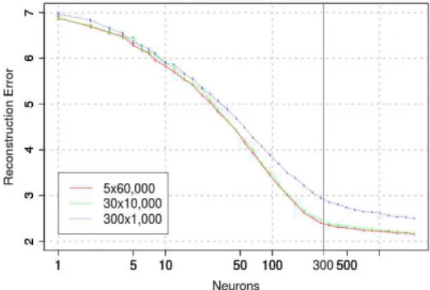
The Reconstruction Error on the MNIST test set for the first RBM is reported vs the number of neurons (in log scale) in Fig.4. As ex-pected, the Reconstruction Error is a monotonically decreasing func-tion of the number of neurons. The feasibility of the approach how-ever is empirically established as the Reconstruction Error displays a plateau when the number of neurons increases5. After these results,
4Mean Field Contrastive Divergence is used in the unsupervised phase, and
backpropagation with momentum is used in the supervised phase. The al-gorithm is available upon request.
5Experiments conducted on the cifar-10 dataset likewise show a decreasing
reconstruction error as the number of neurons increases. Due to the higher complexity of the cifar-10 dataset comparatively to MNIST, the plateau however was not reached for the largest considered networks (up to 12,000 neurons).
the Reconstruction Error criterion suggests a clear and stable hyper-parameter selection of n1≥ n∗1 = 300 neurons.
Figure 4. Reconstruction Error for different numbers of epochs and sizes of the training set (with the same overall number of gradient updates) in the
first layer of a SRBM.
Following the proposed layer-wise approach (section 3.1), we now optimize the size of the second layer, conditionally to the selected size of the first layer. Setting the size of the first layer to n1= 300,
the selection of the optimal number of neurons in the second layer after the Reconstruction Error criterion (Fig. 5), was conducted in the same way as above. Once again, the experimental results show a plateau for the Reconstruction Error criterion after a certain threshold value. The optimal number of neurons on the second layer condition-ally to n1= 300 is obtained for n2≥ n∗2= 200.
Figure 5. Reconstruction Error vs number of neurons in the second-layer of a SRBM, with n1= 300neurons on the first layer.
The stability of the criterion with respect to experimental settings is illustrated on Fig. 4, which shows the Reconstruction Error for three different sizes of the training set and same number of gradient updates. This confirms that the optimal layer size does not depend on the size of the training set, conditionally to the number of gradient updates; this point will be discussed further in section 4.6.
4.4
Efficiency and consistency
The efficiency of the presented approach must eventually be assessed with the classification accuracy. In the previous experiments, RBMs with different hidden layer sizes were trained and evaluated against the Reconstruction Error criterion only. In order to assess their clas-sification performance, a last layer with 10 output neurons is built
on the top of the first RBM-layer (with weights uniformly initialized in[−1, 1]), and a backpropagation algorithm with early stopping is applied on the whole network [3]. Fig. 6 depicts the classification ac-curacy versus the number of neurons in the hidden layer. As shown in Fig. 7, the classification accuracy increases as the Reconstruction Error decreases. Overall, the unsupervised criterion used for model selection yields same performance as that of the best 1-hidden layer neural networks in the literature (1.9%) [3].
Figure 6. Classification accuracy vs number of neurons for different dataset sizes and numbers of epochs.
Figure 7. Classification accuracy vs Reconstruction Error (the higher and the rightmost the better).
A last question regards the consistency of the modular approach, that is, whether simultaneously optimizing several layers yields the same result as sequentially optimizing each layer conditionally to the optimal setting for the previous layers. The global Reconstruction Er-ror on a 2-layer RBM is depicted in Fig. 8, where the first (resp. sec-ond) axis stands for the number of neurons in the first (resp. secsec-ond) layer.
As could have been expected, the Reconstruction Error decreases as the number of units increases; and it is shown to plateau after a suf-ficient number of units in each layer. Furthermore, one cannot com-pensate for the insufficient number of units in layer 1 by increasing the number of neurons in layer 2. This behavior is unexpected in the perspective of the mainstream statistical learning theory [20], where the VC-dimension of the model space increases with the number of weights in the network, whatever the distribution of the neurons on the different layers, as confirmed empirically in the multi-layer per-ceptron framework [18].
The Reconstruction Error isolines are approximately rectangular-shaped: for a given number of units n1on the first layer, there exists a
Figure 8. Overall Reconstruction Error in a 2-layer RBM vs the number of units in first layer (horizontal axis) and second layer (vertical axis). The
white cross shows the optimal configuration found with the layer-wise procedure (300,200).
best Reconstruction Error reached for n2greater to a minimal value,
referred to as n∗2(n1). Likewise, the best Reconstruction Error for a
given number of units n2on the second layer, is reached whenever
the number of hidden units on the first layer is sufficient. Overall, the optimal Reconstruction Error w.r.t. the simultaneous optimization of n1and n2, given in Fig. 8, leads to the same optimal setting as the
layer-wise procedure in Fig.4 and Fig.5 ((n1, n2)∗= (n∗1, n∗2(n∗1)),
which empirically confirms the modularity of the optimization prob-lem.
4.5
Generality
Complementary experiments show that the presented approach hardly applies when considering Contrastive Divergence (instead of Mean Field); on the one hand, the Reconstruction Error very slowly decreases as the number of neurons increases, making the plateau de-tection computationally expensive. Furthermore, the Reconstruction Error displays a high variance between runs due to the stochastic na-ture of the learning procedure.
In the meanwhile, the same approach was investigated in the Auto-Associator (AA) framework, which naturally considers the struction Error as training criterion. Fig. 9 shows the AA Recon-struction Error on the MNIST dataset vs the number of neurons. In-terestingly, the optimal layer size is larger than in the RBM case; interpreting this fact is left for further work.
Figure 9. Reconstruction Error vs number of neurons for an Auto-Associator.
4.6
Model selection and training process
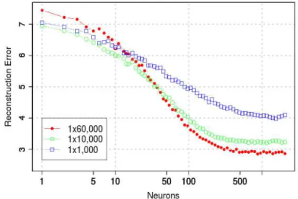
Intermediate experiments, aimed at reducing the computational cost and memory resources involved in the experiment campaign, led to consider datasets with sizes 60,000, 10,000 and 1,000 (Fig. 10) trained for 1 epoch. Quite interestingly, for the Reconstruction Error criterion, the optimal number of hidden units decreases with smaller datasets.
Figure 10. Reconstruction Error vs the number of hidden units in a 1-layer RMB, depending on the size of the training set.
A second experiment was launched to see if the above results could be attributed to the increased diversity of the bigger datasets, or to the increased number of gradient updates (granted that 1 epoch was used for every dataset in Fig. 10).
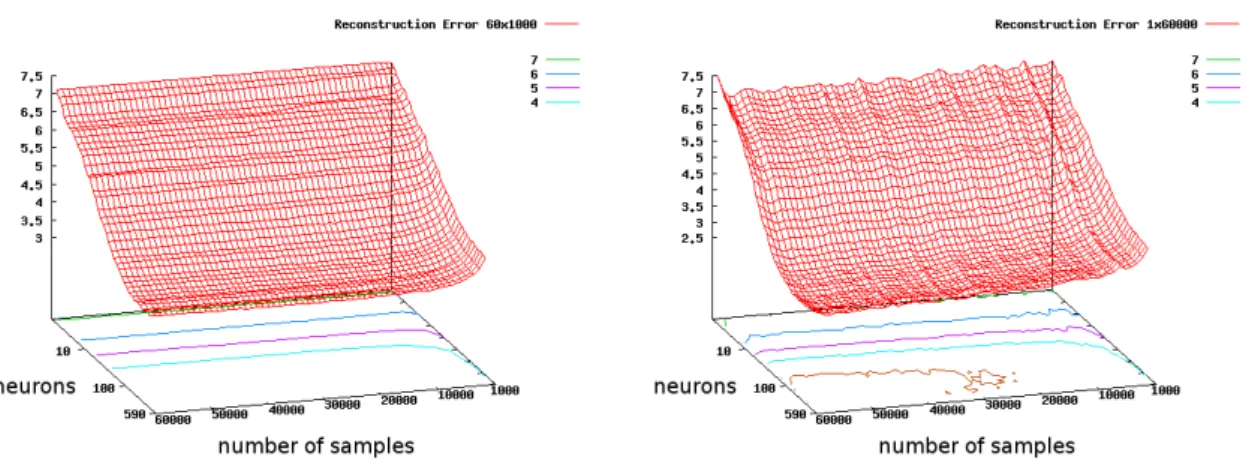
For two datasets of 1,000 and 60,000 samples, the Reconstruction Error is evaluated at multiple points in the training process, each sep-arated by 1,000 gradient updates. The results (Fig.11) show the Re-construction Error w.r.t. the number of neurons for the two datasets as the training progresses from right to left. The Reconstruction Er-ror isolines clearly show the decreasing number of neurons needed with the increasing number of gradient updates.
A tentative interpretation for this fact goes as follows. Firstly, the above results state that the optimal model size can decrease as train-ing goes on. Secondly, a main claim at the core of DNNs [4, 12] is that they capture a more abstract and powerful description of the data domain than shallow networks. Therefore it is conjectured that the network gradually becomes more able to construct key features as training goes on. Further work will aim at investigating experi-mentally this conjecture, by examining the features generated in the deep layers depending on the input distribution, as done by [16].
5
Conclusion and Perspectives
The contribution of the paper is twofold. Firstly, an unsupervised layer-wise approach has been proposed to achieve model selection in Deep Networks. The selection of hidden layer sizes is a critical issue potentially hindering the large scale deployment of DNN. A frugal unsupervised criterion, the Reconstruction Error, has been proposed. A proof of principle for the feasibility and stability of Reconstruc-tion Error-based Model SelecReconstruc-tion has been experimentally given on the MNIST dataset, based on an extensive experiment campaign. The merits of the approach have also been demonstrated from a super-vised viewpoint, considering the predictive accuracy in classification for the supervised DNN learned after the unsupervised layer-wise parameter setting.
Figure 11. Reconstruction Error for RBM trained on 60x1,000 (Left) and 1x60,000 examples (Right) as a function of the number of neurons and gradient updates.
After these results, the model selection tasks related to the differ-ent layers can be tackled in a modular way, iteratively optimizing each layer conditionally to the previous ones. This result is unex-pected in the perspective of standard Neural Nets, where the com-plexity of the model is dominated by the mere size of the weight vec-tor. Quite the contrary, it seems that deep networks actually depend on the sequential acquisition of different “skills”, or representational primitives. If some skills have not been acquired at some stage, these can hardly be compensated at a later stage.
Lastly, the dependency between the model selection task and the training effort has been investigated. Experimental results suggest that more intensive training efforts lead to a more parsimonious model. Further work will investigate in more depth these findings, specifically examining the properties of abstraction of the hidden lay-ers in an Information Theoretical play-erspective and taking inspiration from [16]. Along the same lines, the choice of the examples (curricu-lum learning [5]) used to train the RBM, will be investigated w.r.t. the unsupervised quality of the hidden units: The challenge would be to define an intrinsic, unsupervised, measure to order the examples and construct a curriculum.
ACKNOWLEDGEMENTS
This work was supported by the French ANR as part of the ASAP project under grant ANR 09 EMER 001 04. The authors gratefully acknowledge the support of the PASCAL2 Network of Excellence (IST-2007-216886).
REFERENCES
[1] D.H. Ackley, G.E. Hinton, and T.J. Sejnowski, ‘A learning algorithm for boltzmann machines’, Cognitive Science, 9(1), 147–169, (1985). [2] Y. Bengio and Y. Grandvalet, ‘No unbiased estimator of the variance
of k-fold cross-validation’, Journal of Machine Learning Research, 5, 1089–1105, (2004).
[3] Y. Bengio, P. Lamblin, V. Popovici, and H. Larochelle, ‘Greedy layer-wise training of deep networks’, in Proc. of NIPS’07, eds., B. Sch¨olkopf, J. Platt, and T. Hoffman, 153–160, MIT Press, Cam-bridge, MA, (2007).
[4] Y. Bengio and Y. LeCun, ‘Scaling learning algorithms towards ai’, in
Large-Scale Kernel Machines, MIT Press, (2007).
[5] Yoshua Bengio, Jerome Louradour, Ronan Collobert, and Jason We-ston, ‘Curriculum learning’, in Proc. of ICML’09, (2009).
[6] T.G. Dietterich, ‘Approximate statistical tests for comparing supervised classification learning algorithms’, Neural Computation, (1998).
[7] B. Efron and R. Tibshirani, An introduction to the bootstrap, volume 57 of Monographs on Statistic and Applied Probability, Chapman & Hall, 1993.
[8] Dumitru Erhan, Pierre-Antoine Manzagol, Yoshua Bengio, Samy Ben-gio, and Pascal Vincent, ‘The difficulty of training deep architectures and the effect of unsupervised pre-training’, in Proc. of AISTATS’09, (2009).
[9] T. Hastie, R. Tibshirani, and J. H. Friedman, The Elements of Statistical
Learning: Data Mining, Inference, and Prediction, Springer Series in Statistics, 2001.
[10] G.E. Hinton., ‘Training products of experts by minimizing contrastive divergence’, Neural Computation, 14, 1771–1800, (2002).
[11] G.E. Hinton, S. Osindero, and Yee-Whye Teh, ‘A fast learning algo-rithm for deep belief nets’, Neural Conputation, 18, 1527–1554, (2006). [12] G.E. Hinton and R. Salakhutdinov., ‘Reducing the dimensionality of data with neural networks’, Science, 313(5786), 504–507, (July 2006). [13] H. Larochelle, Y. Bengio, J. Louradour, and P. Lamblin, ‘Explor-ing strategies for train‘Explor-ing deep neural networks’, Journal of Machine
Learning Research, 10, 1–40, (2009).
[14] H. Larochelle, D. Erhan, A. Courville, J. Bergstra, and Y. Bengio, ‘An empirical evaluation of deep architectures on problems with many fac-tors of variation’, in Proc. of ICML’07, pp. 473–480, New York, NY, USA, (2007). ACM.
[15] Nicolas Le Roux and Yoshua Bengio, ‘Representational power of re-stricted boltzmann machines and deep belief networks’, Neural
Com-putation, 20(6), 1631–1649, (2008).
[16] Honglak Lee, Roger Grosse, Rajesh Ranganath, and Andrew Y. Ng, ‘Convolutional deep belief networks for scalable unsupervised learning of hierarchical representations’, in Proc. of ICML’09, p. 77, (2009). [17] V. Mnih, Cs. Szepesvari, and J.-Y. Audibert, ‘Empirical Bernstein
stop-ping’, in Proc. of ICML’08, (2008).
[18] H. Paugam-Moisy, ‘Parallel neural computing based on network dupli-cating’, in Parallel Algorithms for Digital Image Processing, Computer
Vision and Neural Networks, ed., I. Pitas, 305–340, John Wiley, (1993). [19] Robert Tibshirani, Guenther Walther, and Trevor Hastie, ‘Estimating the number of clusters in a dataset via the gap statistic’, Journal of the
Royal Statistical Society B, 63, 411–423, (2000). [20] V. N. Vapnik, Statistical Learning Theory, Wiley, 1998.
[21] M. Welling and G.E. Hinton, ‘A new learning algorithm for mean field boltzmann machines’, in Proc. of the International Conference on
Arti-ficial Neural Networks (ICANN), (2002).