Computational structure analysis of multicomponent oxides

(1)

Computational Structure Analysis of Multicomponent Oxides

by

Yoyo Hinuma

Submitted to the Department of Materials Science and Engineering in partial fulfillment of the requirements for the degree of Doctor of Philosophy in Materials Science and Engineering

at the

MASSACHUSETTS INSTITUTE OF TECHNOLOGY June 2008

Author . . .

Department of Materials Science and Engineering

April 10, 2008

Certified by . . .

Gerbrand Ceder

R. P. Simmons Professor of Materials Science and Engineering

Thesis Supervisor

Accepted by . . .

Samuel Miller Allen

POSCO Professor of Physical Metallurgy

(2)

(3)

Computational Structure Analysis of Multicomponent Oxides

by

Yoyo Hinuma

Submitted to the Department of Materials Science and Engineering on April 10 in partial fulfillment of the requirements for the degree of

Doctor of Philosophy in Materials Science and Engineering

Abstract

First principles density functional theory (DFT) energy calculations combined with the cluster expansion and Monte Carlo techniques are used to understand the cation ordering patterns of multicomponent oxides. Specifically, the lithium ion battery cation material LiNi0.5Mn0.5O2 and the thermoelectric material P2-NaxCoO2 (0.5 ≤ x ≤ 1) are investigated

in the course of this research. It is found that at low temperature the thermodynamically stable state of LiNi0.5Mn0.5O2 has almost no Li/Ni disorder between the Li-rich and

transition metal-rich (TM) layer, making it most suitable for battery applications. Heating the material above ~600oC causes an irreversible transformation, which yields a phase with 10~12% Li/Ni disorder and partial disorder of cations in the TM layer. Phase diagrams for the NaxCoO2 system were derived from the results of calculations making

use of both the Generalized Gradient Approximation (GGA) to DFT and GGA with Hubbard U correction (GGA+U). This enabled us to study how hole localization, or delocalization, on Co affects the ground states and order-disorder transition temperatures of the system. Comparison of ground states, c lattice parameter and Na1/Na2 ratio with experimental observations suggest that results from the GGA, in which the holes are delocalized, matches the experimental results better for 0.5 ≤ x ≤ 0.8. We also present several methodological improvements to the cluster expansions. An approach to limit phase space and methods to deal with multicomponent charge balance constrained open systems while including both weak, long-range electrostatic interactions and strong, short-range interactions in a single cluster expansion.

Thesis Supervisor: Gerbrand Ceder

(4)

Acknowledgments

First of all, I would like to thank my advisor Prof. Gerbrand Ceder for funding, research advice and all the other nice things. I also thank my thesis committee, Prof. Yang Shao-Horn and Prof. Yet-Ming Chiang for helping me improve this thesis, and to Dr. Robert Doe for proofreading the thesis document.

My computational work was greatly helped by cluster expansion and Monte Carlo code by Dr. Anton van der Ven and Dr. Tim Mueller. Dr. Ying Shirley Meng helped me with scientific discussion and improvement of my paper writing and survival skills. I also appreciate my past and present lab mates and other people at MIT who made my life here a great experience.

Finally, I would like to thank my daughter Sumika for being a nice kid while daddy was working on his thesis, and my wife Junko for supporting and encouraging me.

(5)

(We) can’t reach (the goal) unless (we) mistake correctly… Wait! If (we) correctly mistake, (we) can reach (the goal)!

(6)

Chapter 1 Introduction

Altering the properties of materials always requires a change in the local environment of the atoms within the material. For example, doping creates some atomic environments that include the dopant as neighbors, while annealing enables more frequent atomic diffusion that results in new, energetically favorable atomic environments at the annealing temperature. Quenching differs from slow cooling because atomic environments favored in high temperature are more likely to remain after cooling. These examples illustrate how many different local structures can be obtained during the experimental process, some being more energetically favorable than others.

It should be possible to make materials with ideal properties if the optimum atomic environments and corresponding processing conditions are known. The primary problem is that an understanding of the atomic environments cannot be easily obtained or measured except in the simplest systems; thus atomic scale engineering is not commonly utilized as a means of property improvement or control. Currently, a variety of experimental methods such as X-ray diffraction (XRD), nuclear magnetic resonance (NMR), transmission electron microscopy (TEM) and X-ray absorption fine structure spectroscopy (XAFS) are utilized to probe different length scales, yielding some idea of the environments. Computational methods such as first principles density functional theory (DFT) are being utilized to conduct total energy calculations with full structural

(9)

relaxation from an arbitrary initial configuration. However due to computational restrictions the unit cell size is limited, in turn limiting the description of long range order in a system.

Some systems with structural disorder may be very difficult to understand using experimental techniques. Lithium transition metal oxides such as LiNi0.5Mn0.5O2 or

LiNi1/3Co1/3Mn1/3O2 are one example: XRD or electron diffraction cannot distinguish the

transition metals in these materials because they have a similar number of electrons. However, structural disorder can be precisely controlled in computation, where arbitrary unit cells can be used as input.

In this thesis, a computational “atomic engineering” approach is used to gain insight into the optimal material (phase) for a specific use of a system in consideration. Figure 1-1 shows a schematic flow chart of this approach. First, energies (EFP) of various

atomic configurations (σ) are obtained using first principles methods. Next, the cluster expansion formalism is used to fit the first principles energies to a simple polynomial of occupation variables on sites within a lattice model. It is also possible to understand the relevant interactions between atoms of the system in consideration from the cluster expansion. Afterward, Monte Carlo simulation is conducted to quickly sample energies of large unit cells using relatively accurate energies (ECE) from the cluster expansion

(10)

temperature (T) - composition (x) space. Finally, physical intuition of the system is used to gain insight into processing conditions or composition ranges for possible property improvements. This method should allow us to overcome the unit cell size restriction in DFT while retaining a useful degree of accuracy.

Figure 1-1. Schematic flow chart of properties optimization based on an atomic engineering approach.

This work is composed of explicit application of computational atomic engineering in two systems relevant from both engineering and science viewpoints: in the

(11)

NaxCoO2. This is also the first work to address cluster expansion in restricted phase space

(penalized cluster expansion). Specifically, some atomic configurations were not allowed in each system studied because of too high energy results from the repulsion or overlap of atoms. This restriction was resolved by introducing a penalty to discourage sampling in restricted phase space during the Monte Carlo simulations.

The outline of this thesis is as follows: Chapter 2 covers the general methodology of phase diagram generation while the atomic engineering approach is applied to LiNi0.5Mn0.5O2 and NaxCoO2 in Chapter 3 and Chapter 4 respectively. The

methodological details specific to each system (semi-canonical binary-ternary coupled penalized cluster expansion for LiNi0.5Mn0.5O2, and charge constrained grand canonical

binary or binary-binary coupled penalized cluster expansion for NaxCoO2) are described

in Chapters 3 and 4. The main objective of Chapters 3 and 4 is to understand the relevant physics and obtain a phase diagram showing the thermodynamically stable phases for each of these systems. Finally, Chapter 5 includes concluding remarks, and ideas regarding the direction of future work are presented in Chapter 6.

(12)

Chapter 2 Computational phase diagram generation

2.1 Overview

A temperature-composition (T-x) phase diagram is a key component in the atomic engineering approach because it is used to show what phases, or structures, are thermodynamically stable at a given temperature and composition. First principles calculations (Density Functional Theory: DFT) is a very powerful method of obtaining accurate ground state energies. However, one drawback previously mentioned is computing power limiting the size of the unit cell to roughly ~102 atoms, while another detriment is the inability of DFT to predict accurate energy at finite temperature. Cluster expansion (1) is one possible method of gaining insight into partially disordered states at finite temperatures. Its use has been demonstrated in alloy systems (1-9) as well as Li-vacancy ordering studies in lithium transition metal oxide systems (10-13). In general, the process of cluster expansion involves fitting DFT energies to a simple polynomial (cluster expansion) in order to quickly obtain energies of large cells on the order of ~105 atoms. Additionally, finite temperature behavior can be investigated by combining Monte Carlo simulations with cluster expansion.

It is necessary to conduct the following steps, summarized as a schematic flow chart in Figure 2-1, in order to generate a phase diagram:

(13)

1) First, parameterize the degrees of freedom and obtain the configurational information regarding the structures, then coarse grain out vibrational, electronic and magnetic information (14). The exception to this rule occurs when a single element must be configured with different valences (e.g. ordering of Co3+ and Co4+) or different magnetic spin (e.g. ordering of Ni2+ with up-spin and down-spin). Although the element is the same, if this is an issue that cannot be neglected, then these have to be treated as different species.

2) Decide which structures (ordering patterns) will be considered in fitting the cluster expansion.

3) Obtain first principles energies for each of the structures. The lattice parameters and atomic coordinates will be relaxed in the first principles calculations.

4) Construct a cluster expansion.

5) Complete Monte Carlo simulations with the Metropolis algorithm.

6) If the cluster expansion does not seem to be a good model of the system, then iterate again from step 1.

7) Obtain phase transition temperatures from the simulated energy and/or heat capacity as a function of temperature. As described in detail later, this step may require free energy integration.

8) If grand canonical calculations are conducted, then stable phases for a given temperature may be obtained by observing discontinuities in composition as a function of chemical potential.

(14)

Figure 2-1. Schematic flow chart of phase diagram generation.

The key assumption is that configurational entropy causes the most significant energetic difference between various phases, while the contribution to free energy from other sources of entropy (e.g. vibrational, magnetic and electronic) is insignificant between phases and can be ignored (coarse grained out) (14). However, it should be noted that the fully relaxed energy for a given configuration is used as the energy for a configuration of species in ideal sites on the lattice model. It is possible to extend this formalism to incorporate other entropy sources. For instance, the formalism where vibrational entropy is also taken into consideration is shown in Garbulsky and Ceder (15).

(15)

Details of the cluster expansion construction, Monte Carlo simulation and free energy integration are discussed in the following section 2.2.

2.2 Cluster expansion 2.2.1 Formalism (1)

We consider a lattice model system with N sites where m species can occupy each site. There are mN possible configurations (σ), and we assume the energy (Eσ)is known for each σ. An mN-dimensional vector (φ(σ)) is defined where the components are all possible combinations of one out of (1, σi, σi2 … σim-1) multiplied over all i. Here, i is the

label of a site, and σi is the occupation variable of site i. For example, if N = 2 and m = 3,

i can be either 1 or 2, and one definition of φ(σ) is

φ(σ) = (1, σ1, σ2, σ12, σ1σ2, σ22, σ12σ2,σ1σ22, σ12σ22). (2.1)

Occupation variables can take m different values depending on what species is occupying the site i (one example for values of the occupation variables are integers 0, 1, 2 … m−1). An mN-dimensional vector (V) exists such that Eσ is obtained by

Eσ = V•φ(σ). (2.2) Going back to the N = 2 and m = 3 example, if the occupation variables for site i are defined as σi = 0 if species A is occupying site i, 1 if species B is occupying and 2 if

(16)

φ(AA) = (1, 0, 0, 0, 0, 0, 0, 0, 0)

φ(AB) = (1, 0, 1, 0, 0, 1, 0, 0, 0)

φ(BC) = (1, 1, 2, 1, 2, 4, 2, 4, 4). (2.3) For

V = (V00, V10, V01,V20,V11,V02,V21,V12,V22) (2.4)

examples of relations obtained by combining equation 2.2 with equations 2.3 and 2.4 are:

EAA = V00

EAB = V00 + V01+ V02

EBC = V00 + V10 + 2V01 +V20 + 2V11 + 4V02 + 2V21 + 4V12 +4V22 (2.5)

It is possible to uniquely calculate the explicit value of V by solving the full set of equations such as those in equation 2.5. It is important to note that values of V do not have any meaning unless the corresponding occupation variables are specified.

In the case of a coupled system with two sublattices, where there is an additional sublattice with N’ sites and m’ species, m’N’ possible configurations (τ) exist. Defining j as the sites and τj as the occupation variables on the additional sublattice as, φ(σ,τ) is

defined as a mNm’N’-dimensional vector where the components are all possible combinations of products of (1, σi, σi2 … σim-1) over all i and (1, τj, τj 2 …τj m’-1) over all i.

Eστ is obtained by

(17)

It is possible to expand this formalism to systems with three or more sublattices in a similar way.

Now we attempt to simplify the cluster expansion using symmetry of the lattice. For simplicity, we can assume a system with one sublattice and m = 2, which is the case for a binary system. This enables equation 2.2 to be rearranged based on the total number of σi in each term: L + + + + =

∑

ijk ijk i j k ij ij i j i i i V V V V E ₀ σ σ σ σ σ σ (2.7)

where i, j, k indicate different sites. As seen in the previous example, when m > 2, terms

with squares and higher powers of σi will appear (equation 2.1) (16). Also note that in a

coupled system some terms include products of both σi and τj (17). When sites are

symmetrically equivalent, for example if the sites are on a simple hexagonal lattice, equation 2.7 can be greatly simplified. If all the sites are symmetrically equivalent, Vi no

longer depends on the site i, thus the index can be dropped. The set of coefficients V,

named effective cluster interactions (ECI), may be regarded as a function of the relevant cluster, or configuration of sites. Similarly, the number of independent coefficients for pair clusters (clusters involving two sites) or triplet clusters (clusters with three sites) may be drastically reduced.

(18)

2.2.2 Cluster expansion approximation for energy prediction

The cluster expansion formalism in section 2.2.1 is exact, and in principle the cluster expansion (e.g. equation 2.7) has to be summed over all pairs, triplets, quadruplets, and larger clusters of sites. However, in practice the cluster expansion can be used to approximate the energy of a complicated system with very few coefficients. The ECI can be regarded as the effect of interactions in the cluster on the total energy. Therefore irrelevant clusters, such as those that include long-distance pairs, or contain too many sites, can be removed from the cluster expansion (ECI set to zero).

The main difficulty in making a good cluster expansion approximation is choosing which clusters to include in the cluster expansion and in choosing which structures to include when fitting (training) the cluster expansion. Relevant clusters are selected on the basis of how well they minimize the weighted cross-validation (CV) score. This is a means of describing how good the cluster expansion is at predicting the energy of a structure not included in the fit (18). A large number of structures close to the convex

hull, or the line connecting the minimum energy possible in a given composition, should be calculated since it is crucial to obtain the correct ground states, and an accurate energy scale of the low energy excitations, to compile an accurate phase diagram. These low energy structures should also be weighed heavily when obtaining the CV score. Some structures with large excitation energies are also necessary to “pin” at high energy

(19)

structures in the cluster expansion so the local environments of high energy structures do not form in the Monte Carlo simulations. These high energy structures may be weighed lightly since it is not necessary to accurately predict the energy of these structures as compared to structures with lower energy.

It is crucial to have some insight into the physics of the system when determining the form of the cluster expansion. For example, if there are noticeably strong interactions, the ECI for clusters that represent such interactions should have larger magnitude. In general, larger clusters should have ECI of less magnitude than the ECI for smaller clusters, as well as a small ECI for clusters near the truncation cutoff. There are some cases, such as NaxCoO2 discussed in Chapter 4, where there are long-range electrostatic

interactions that cannot be truncated to a short distance, necessitating a large number of pair clusters. To capture the physics of these systems, the energy from “background” ECIs representing the electrostatic interactions is removed prior to fitting the DFT energies to the cluster expansion, and then added back to the fitted cluster expansion.

When parts of the phase space are inaccessible or accurate energies are hard to obtain (e.g. if the simultaneous occupancy of nearest-neighbor pair is prohibited), it is possible to remove affected clusters thus removing any resulting linear dependencies in the fitting. Then, a penalty on the cluster expansion is added to increase the energy of the system in the restricted phase space. The penalized cluster expansion is applied to the

(20)

LiNi0.5Mn0.5O2 system and NaxCoO2 system in Chapters 3 and 4 respectively, and there

the actual forms of the cluster expansions are shown.

2.3 Monte Carlo simulation

Monte Carlo simulation is an efficient method to understand finite temperature behavior. The most common algorithm is the Metropolis algorithm (19) where

perturbations to the system are accepted or denied according to the following criteria: 1) If Hold ≥ Hnew, then accept the perturbation

2) If Hold < Hnew and exp rand

( )

0,1

kT H H_new _old <       −

− , then accept the perturbation

3) Else, deny the perturbation.

Here, Hold and Hnew are the Hamiltonian values of the original (old) and perturbed (new)

systems, k is a coefficient (Boltzmann constant), T is the temperature and rand (0,1) is a

random number between 0 and 1 (0 and 1 exclusive) that is generated every time a perturbation is considered.

The perturbation is always accepted when it lowers the Hamiltonian (energy) and is sometimes accepted when the perturbation increases the energy; the likelihood exponentially decreasing with increase in energy. When implementing this method, it is crucial to not allow 0 as the random number to prevent any perturbation from being

(21)

If a grand canonical Monte Carlo simulation is being conducted, the Hamiltonian is the thermodynamic potential defined as

N E−µ =

Ω . (2.8) Here, E is the energy, and µ is the chemical potential for the relevant composition N.

Although a variety of perturbations are allowed to be used (e.g. simultaneously changing multiple occupation variables that conserve charge balance), the simplest perturbation is changing the occupation variable of one site. Such grand canonical simulation is the preferred method when composition is allowed to change because no two-phase regions appear in a temperature-chemical potential (T-µ) phase diagram. Two-phase regions do appear in the T-x phase diagram because discontinuity of composition is allowed at

first-order phase transition boundaries.

Monte Carlo simulations are typically conducted with either fixed temperature or fixed chemical potential to scan T-µ phase space. The correlation length and correlation time of the system diverges close to phase transitions (20). Finite size effects are

observed near transitions because the correlation length is limited to the Monte Carlo cell dimensions. For example, the magnitude of peaks in the thermodynamic potential fluctuation (e.g. heat capacity) changes with system size. First order transitions, such as some order-disorder transitions, are detected when E or the slope of Ω is discontinuous. The heat capacity cannot be defined at the transition point, however a peak is often observed. Second-order transitions, such as some order-order transitions, have continuous

(22)

E at the transition point and are characterized by the peak in the fluctuation that changes

with the system size.

Free energy integration is needed when the phase transition temperature cannot be simply be obtained from the energy and/or heat capacity calculated during Monte Carlo simulations. One example occurs when there is a significant hysterisis between grand canonical heating and cooling runs at the same chemical potential, as seen in the next section.

2.4 Free energy integration

In thermodynamics, the free energy of a system with one compositional degree of freedom F (T, N) is defined as

Q kT

F =− ln (2.9) where k is the Boltzmann constant. The partition function

(

)

∑

− = σ σ βE Q exp (2.10)

is summed over all configurations (σ). Here, β is equal to (kT)1.

The Legendre transformation is used to obtain the free energy

( )

T µ =F−µN

Φ , (2.11) for Ω. Φ is given by:

(23)

Z kT ln

− =

Φ (2.12) using the (grand canonical) partition function:

( )

_∑

(

)

_∑

(

)

σ σ σ σ σ Ω β − = µ − β − = µ β, exp E N exp Z . (2.13)

Free energy integration can be conducted when the free energy (Φ0) is known for

a given temperature (T0) and chemical potential (µ0). The free energy F (Φ) is equivalent

to the energy E (Ω) when there are no excitations (T = 0 or entropy S = 0), and these points are useful as primary reference points. The following integration methods can be used to obtain the free energy for other points:

1) Along a fixed temperature trajectory,

(

)

(

)

(

)

(

E N

)

N N E N kT Z kT T T − = µ − β − µ − β − β − =       µ ∂ ∂ − =       µ ∂ Φ ∂

∑

σ σ σ σ σ σ σ exp exp ln (2.14)

where N is the grand canonical thermodynamical average of N. Integrating equation 2.14 leads to:

(

µ

)

=Φ

(

µ

)

−

(

µ

)

µ Φ

_∫

µ µ N T d T T 0 , , , ₀ ₀ ₀ 0 . (2.15)

2) Along a fixed chemical potential trajectory,

( )

(

)

(

−βΩ

)

= Ω Ω β − Φ =       β ∂ ∂ − =       β ∂ β Φ ∂

∑

σ σ σ σ σ µ µ exp exp ln Z (2.16)

(24)

(

)

Φ

(

µ

)

₊ _Ω

₍

_µ

₎

_β = µ Φ

∫

T d kT T kT T T T0 0 0 0 0 0 , _, , . (2.17)

These integrations are typically conducted numerically by trapezoidal summation, represented as:

( )

( ) ( ) (

₁

)

1 1 2 0 ₌ − − _⋅ ₋ + =

∑

∫

i i k i i i x x x x x f x f dx x f k . (2.18)

Figure 2-2 depicts two representative phase diagrams with the free energy integration trajectories shown as bold lines in the T-µ phase diagram in Figure 2-2a. The phase transition point is where F (for canonical calculations) or Φ (for grand canonical calculations) of the low temperature phase and high temperature phase equal. For the low temperature phase, method 2 is used to obtain Φ by integrating Ω of a fixed chemical potential heating simulation from a low enough temperature (equation 2.17). For the high temperature phase, method 1 is used to obtain a reference free energy at Thigh with a fixed

temperature calculation (equation 2.15). Afterward, method 2 can be utilized to integrate

Ω of a fixed chemical potential cooling simulation (equation 2.17). Figure 2-2b shows the trajectories in T-x space, and how the discontinuity in concentration at the phase transition point leads to a two-phase region.

(25)

Figure 2-2. Schematic phase diagram in (a) temperature-chemical potential space and (b) temperature-composition space. Free energy integration trajectories are shown with arrows.

Figure 2-3 shows an actual simulation result demonstrating phase transition temperature determination from free energy integration in NaxCoO2. The grand canonical

energy (Ω) as a function of temperature obtained from Monte Carlo simulation are shown in Figure 2-3a. The phase transition temperature is between 430K (transition observed from cooling simulation) and 480K (transition observed from heating simulation), but cannot be obtained with higher precision unless there is other information. In contrast, the phase temperature is determined accurately as 450K from the free energy (Φ) as a function of temperature in Figure 2-3b because the free energies of cooling and heating simulations intersect at this point.

(26)

Figure 2-3. Demonstration of phase transition temperature from free energy integration. (a) Grand canonical energy (Ω) from Monte Carlo simulation. (b) Free energy (Φ) obtained from the energies in (a).

(27)

2.5 References

1. J. M. Sanchez, F. Ducastelle, D. Gratias, Physica A: Statistical and Theoretical

Physics 128, 334 (1984).

2. D. de Fontaine, in Solid State Physics - Advances in Research and Applications. (1994), vol. 47, pp. 33-176.

3. G. Ceder, A. Van der Ven, C. Marianetti, D. Morgan, Modelling and Simulation in

Materials Science and Engineering 8, 311 (May, 2000).

4. M. Asta, S. M. Foiles, A. A. Quong, Physical Review B 57, 11265 (May 1, 1998). 5. C. Wolverton, Philosophical Magazine Letters 79, 683 (Sep, 1999).

6. V. Ozolins, B. Sadigh, M. Asta, Journal of Physics-Condensed Matter 17, 2197 (Apr 6, 2005).

7. M. Asta, V. Ozolins, C. Woodward, Jom-Journal of the Minerals Metals &

Materials Society 53, 16 (Sep, 2001).

8. C. Wolverton, D. Defontaine, Physical Review B 49, 8627 (Apr 1, 1994). 9. M. Asta, C. Wolverton, D. Defontaine, H. Dreysse, Physical Review B 44, 4907

(Sep 1, 1991).

10. A. Van der Ven, M. K. Aydinol, G. Ceder, G. Kresse, J. Hafner, Physical Review B

58, 2975 (1998).

11. C. Wolverton, A. Zunger, Physical Review Letters 81, 606 (Jul 20, 1998).

12. C. Wolverton, A. Zunger, Journal of the Electrochemical Society 145, 2424 (Jul,

1998).

13. M. de Dompablo, A. Van der Ven, G. Ceder, Physical Review B 66, 64112 (Aug 1, 2002).

14. G. Ceder, Computational Materials Science 1, 144 (1993).

15. G. D. Garbulsky, G. Ceder, Physical Review B 53, 8993 (Apr 1, 1996).

16. G. Ceder, G. D. Garbulsky, D. Avis, K. Fukuda, Physical Review B 49, 1 (Jan 1, 1994).

17. P. D. Tepesch, G. D. Garbulsky, G. Ceder, Physical Review Letters 74, 2272 (Mar 20, 1995).

18. A. van de Walle, G. Ceder, Journal of Phase Equilibria 23, 348 (Aug, 2002). 19. N. Metropolis, A. W. Rosenbluth, M. N. Rosenbluth, A. H. Teller, E.Teller,

Journal of Chemical Physics 21, 1987 (1953).

20. N. E. J. Newman, G. T. Barkema, Monte Carlo Methods in Statistical Physics (Clarendon Press, Oxford, 1999), pp. 83-85.

(28)

Chapter 3 The lithium battery material Li

x

Ni

0.5

Mn

0.5

O

2

3.1 Introduction to lithium ion batteries

Batteries are charge storage devices in which electrical energy can be extracted from a chemical reaction known as discharging. In the case of a secondary, or rechargeable, battery the reaction chemistry is reversible and the charge can also be restored (charged). When a battery is charged or discharged electrons move from one electrode to the other through an external circuit in order to store or release energy. The two electrodes, referred to as the cathode and anode, are electronically separated by a separator (e.g. polypropylene sheets) in the battery. Electron transfer through the external circuit of the cell is compensated by ionic transfer through the electrolyte between the electrodes.

Figure 3-1 shows the dependency of energy density on the various battery chemistries. Among these, lithium ion (Li-ion) batteries exhibit the highest theoretical energy density (1). For this reason, Li-ion batteries are an attractive choice for applications where space and weight constraints are stringent, such as in portable electronics and space applications. In Li-ion batteries, this charge transfer is done by Li+ diffusion. The first commercialized rechargeable Li-ion battery was released by Sony in June 1991. The cell chemistry consisted of graphite anode combined with a high

(29)

temperature phase of lithium cobalt oxide (HT-LiCoO2, or simply LiCoO2) as the cathode

(2).

Figure 3-1. Comparison of the different battery technologies in terms of volumetric and gravimetric energy density (1).

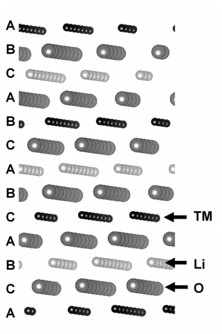
HT-LiCoO2 has a layered O3 structure (3) as shown in Figure 3-2. If all the

cations consist of the same element, then this is equivalent to the rocksalt structure. However, LiCoO2 consists of alternating Li and transition metal layers that form along

(30)

Figure 3-2. Lithium transition metal oxide (LiTMO2) in the O3 structure. In LiCoO2, all

transition metals are Co.

The most important feature of the O3 lithium transition metal oxide family is that the Li layer acts as a two-dimensional Li+_{diffusion channel, allowing Li}+_{to be}

(31)

inserted and removed with relative ease. The activation barrier to Li+ diffusion within this channel is reported to be about 200meV, or about 8kBT at room temperature from first

principles calculations (4).

One major drawback of LiCoO2 is that the usable capacity is ~150mAh/g,

roughly half of its theoretical capacity. This is because discharge above this threshold, or overdelithiation, causes a sudden decrease in the c lattice parameter (5, 6) due to a phase transition from the O3 phase to the H1-3 phase (6, 7). Upon further discharge, there is another phase transition to the O1 phase (6, 7). There are also safety issues with LiCoO2,

since Li0.4CoO2 has been shown to release oxygen upon heating to ~200oC (8). This

oxygen can combust the organic electrolyte and lead to a rapid battery fire.

During the search for next-generation Li-ion battery cathode materials, Co was replaced by other transition metals including Ni or Mn. When compared with LiCoO2,

LiNiO2 shows less thermal stability as a cathode material (8). The thermodynamically

stable phase of LiMnO2 is not the O3 rocksalt structure, and Li+ removal causes

irreversible structural transformation, forming a less electrochemically active phase (9). To circumvent problems like these, a combination of transition metals has been used to substitute Co. Two promising materials that have exhibited significantly better stability are LiNi1/3Co1/3Mn1/3O2 and LiNi0.5Mn0.5O2. LiNi1/3Co1/3Mn1/3O2 has capacity of

(32)

versus Li+/Li (10). LiNi0.5Mn0.5O2 also has higher reversible capacity of about 200mAh/g

by charging to 4.5V (11-14).

3.2 Characteristics of LiNi0.5Mn0.5O2

LiNi0.5Mn0.5O2 (11-16) is an interesting material for both its engineering and

scientific aspects. As mentioned in the previous section, the theoretical capacity of LiNi0.5Mn0.5O2 is about 280 mAh/g, of which 200 mAh/g can now routinely be achieved

at low rates such as C/20 (11-14, 16). Moreover, since LiNi0.5Mn0.5O2 does not contain

the rather expensive cobalt, a reduction of cost for Li batteries may be realized with this material. Other properties of the material, such as thermal stability and safety, have also been demonstrated to be better than LiCoO2 (11, 13).

Though the rate capability of the material has generally been shown to be poor, recent efforts indicate that it may be possible to overcome this issue by structural modifications (16), keeping this an attractive electrode material. Much of the desirable properties are derived from the synergetic combination of Mn4+ and Ni2+. Mn4+ is one of the most stable octahedral ions, maintaining the structural integrity when Li is extracted, while Ni2+ can be fully oxidized to Ni4+, thereby compensating for the fact that Mn4+ cannot be oxidized further (17-19).

(33)

On average, the cation positions of LiNi0.5Mn0.5O2 are characterized as the

O3-type layered structure (20) similar to LiCoO2, however elucidating the details of the

cation ordering has been difficult (12, 21-27). In addition, there is a significant correlation between structure and electrochemical performance, which becomes clear when comparing different synthesis conditions. For instance a small amount of Ni in the Li layers is always observed in materials synthesized at temperatures around 900~1000oC with conventional solid state processes. In general, there is about 8~11% of this type of Li/Ni disorder (11, 13, 21, 23, 24, 28-32). Some literature suggests that Li/Ni disorder will increase slightly as annealing temperature is decreased (13, 28).

Li/Ni disorder has negative effects on deintercalation of Li+ (16) because Ni atoms positioned in the Li layer reduce the region of space in which Li+ diffuses, resulting in an increased Li+ diffusion activation barrier and reduced rate capability (16). As a result, there is an incentive to find methods to move these Ni into the TM layer and to investigate whether Ni is mobile during delithiation. Earlier XAFS results from a study by Arachi et al (21) suggest migration of Ni into tetrahedral sites, though the details of the mechanism are not known. Van der Ven and Ceder (25) succeeded in developing a reasonable first principles model of the delithiation voltage, however, in their model, a perfect “flower” ordering was assumed for transition metals, and no transition metal movement was allowed during delithiation (25).

(34)

The valence states of Ni and Mn are observed to be +2 and +4 respectively in both first principles computation (32) and X-ray absorption spectroscopy (33, 34). Thus, electrostatic interactions are likely to have a strong effect on the ordering of Ni and Mn in the Transition Metal-rich layer (TM layer). Four different structural models of the TM layer in LiNi0.5Mn0.5O2 have been proposed by various theoretical and experimental

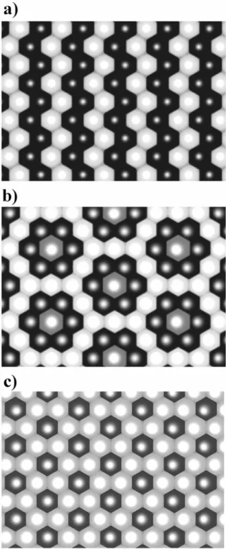
investigations: 1) The zigzag structure (30) in which Mn and Ni are ordered in zigzag lines without any significant amount of Li present in the TM layer (Figure 3-3a); 2) the

flower structure with a 2√3 × 2√3 unit cell, which consists of concentric hexagons of Mn and Ni around a central Li (Figure 3-3b) (25); 3) the partially disordered honeycomb structure with √3 × √3 unit cell (23) in which the symmetry is broken between a Mn-rich and a Li-rich sublattice (Figure 3-3c) (35); and 4) a disordered model without any particular ordering between Mn and Ni (28). The honeycomb model seems to agree best with the available experimental evidence. Experiment suggests that two types of sites, denoted α and β, compose the TM layer (23). The α sites are generally occupied by either Li or Ni, while the β sites are preferred by Ni or Mn. The α sites are always the nearest neighbors to a β site. The flower structure is commensurate with the honeycomb model, but it displays a higher degree of long-range order, and can be considered a special case of the honeycomb model. Understanding cationic arrangement in this material is important as the electrochemical lithiation/delithiation process and the subsequent structural stability depends on the initial structure as suggested from Nuclear Magnetic Resonance (NMR) and first principles studies (25, 31).

(35)

This chapter first shows how Li/Ni disorder limits technologically important factors such as rate capability and capacity. Second, computational evidence of a complex thermal disordering process is presented to show how the system undergoes a phase transition from a low temperature zigzag-like state with no Li/Ni exchange to a partially disordered flower structure with increased temperature. The initial phase change is followed by further disordering which creates a honeycomb superstructure at higher temperature.

(36)

Figure 3-3 (a) Transition Metal layer (TM layer) ordering of the zigzag structure. There is no Li in the TM layer. (b) TM layer ordering of the flower structure. There is 8.3% Li/Ni disorder, or 8.3% Li in the TM layer. Legend: black: Mn, white: Ni, gray: Li. (c) TM layer ordering of the honeycomb pattern. Legend: dark gray: α sites that can be occupied by Li or Ni, light gray: β sites that can be occupied by Ni or Mn.

(37)

3.3 Methodology

Calculations were performed on various ordered arrangements (7, 25, 36-38) utilizing the Generalized Gradient Approximation and Hubbard U correction within Density Functional Theory (GGA+U). Core electron states were represented by the Projector Augmented-Wave method (39) as implemented in the Vienna Ab Initio Simulation Package (VASP) (40). The Purdew-Burke-Ernzenhof (PBE) exchange correlation (41) and a plane wave representation for the wavefunction with a cutoff of 370 eV were used. The Brillouin zone was sampled with a mesh including the gamma point. A 3 x 3 x 3 mesh was used for the flower configuration unit cell with 48 atoms, and for cells with different sizes a mesh with similar density was used. The charge density was spin polarized, with Mn spins aligned ferromagnetically with other Mn, and antiferromagnetically with Ni in the transition metal layer. The moment of Ni in the Li layer was aligned ferromagnetically with Mn. These spin configurations are similar to those suggested in the flower structure (25). The Hubbard U values applied to the Hamiltonian were needed to correct for the self-interaction error that occurs with transition metals with DFT (42, 43). These values have been calculated elsewhere to be 5eV per Mn atom and 5.96eV per Ni atom (42).

A binary-ternary coupled cluster expansion (44) was used to model partially disordered states at finite temperatures. Li and Ni were allowed to occupy sites in the Li

(38)

layer creating binary disorder, whereas ternary disorder was modeled by allowing Li, Ni and Mn to occupy sites in the TM layer. The site variables are designated as τ = 0 for Li and τ = 1 for Ni in the Li layer, and σ = –1 for Mn, σ = 0 for Ni, and σ = 1 for Li in the TM layer. The Hamiltonian becomes:

(3.1) Here, V are the Effective Cluster Interactions (ECI), and V0 specifically acts as a site

energy of the Li layer sites. The ECI VLi, Vint and VTM represent respectively Li layer clusters, clusters that contain both Li and TM layer sites, and TM layer clusters respectively. The indices i, j, and k are labels of sites in the cluster. The dummy indices s,

t, and u are used to distinguish different ECI on the same cluster and are either 1 or 2. The

cluster expansion was fitted to the energies of 183 different configurations of Li, Ni and Mn.

Canonical Monte Carlo simulations were conducted with this cluster expansion in cells of 2592 formula units (2592 Li layer sites, 2592 TM layer sites). In general, 50,000 equilibrium passes and 100,000 sampling passes were used at every temperature between 200K and 1500K. In the range near the phase transitions (700-990K), 100,000

(39)

equilibrium passes were used to allow better equilibration. Note that one sampling pass amounts to one possible perturbation of each site on the lattice.

3.4 Results

3.4.1 Comparison of GGA and GGA+U

The energy of the flower (25) and zigzag (30) structures were calculated with both the GGA and GGA+U approximations to investigate the energy difference between structures with and without Li/Ni disorder. These structures are representative of the limiting states with (flower) and without (zigzag) Li/Ni disorder. Table 3-1 shows the energy differences between the two structures. Note that the energy difference in the two structures is an order of magnitude smaller in GGA than in GGA+U. This is consistent with prior work suggesting that the flower and zigzag structures are almost degenerate in the GGA approximation (25). Though further discussion will follow, all energies used for the cluster expansion fit were calculated with the GGA+U approximation because this method is believed to be a more accurate description of the system.

(40)

Table 3-1. Difference in energy in meV/FU between GGA and GGA+U approximations for flower and zigzag structures.

3.4.2 Delithiation behavior of LixNi0.5Mn0.5O2

First principles energy calculations were conducted on LixNi0.5Mn0.5O2 for

structures with TM layer cations in the flower ordering and zigzag ordering in an effort to understand the difference in delithiation behavior. The energies pertaining to the two scenarios of the flower ordering with 8.3% Li/Ni exchange were calculated, one where diffusion of the Ni in the Li layer to the TM layer was allowed, and another where it was not allowed.

Figure 3-4 shows the convex hull resulting from formation energies of partially delithiated LixNi0.5Mn0.5O2. Formation energies are the energy difference between the

mixed state and a compositionally averaged combination of lowest energy states of Li1Ni0.5Mn0.5O2 and Ni0.5Mn0.5O2. Delithiation of the flower structure causes the Li+ in

the TM layer, and one Li+ in the Li layer, to move into the tetrahedral sites adjacent to the

GGA (∆E) GGA+U (∆E) Flower 0 (Ground state) 26 Zigzag 2 0 (Ground state)

(41)

octahedral site that was previously occupied by Li+ in the TM layer. This forms a dumbbell-like pattern that vacates all Li in octahedral sites adjacent to the two tetrahedral Li+. These pairs of Li+ in the tetrahedral sites are the last Li to be removed during delithiation (25, 45). Ni in the Li layer will not diffuse to the TM layer until the end of delithiation, which is also when tetrahedral Li is removed, even when the diffusion of Ni in the Li layer of flower ordering is allowed. Our findings indicate that TM cation migration is never energetically favorable during delithiation of zigzag ordered LixNi0.5Mn0.5O2.

(42)

Figure 3-4. Formation energies from first principles calculations of partially delithiated LixNi0.5Mn0.5O2. When cations in the TM layer was arranged in the flower ordering,

energies were calculated in the two scenarios where diffusion of the Ni in the Li layer to the TM layer upon delithiation was allowed (with Ni diffusion) or not allowed (no Ni diffusion). One FU contains one transition metal atom.

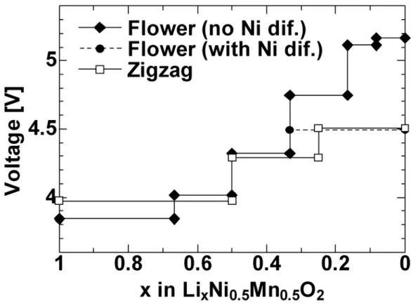
Initial ordering and different scenarios of Ni migration have dramatic effects on the Li deintercalation potential, because the potential is the derivative of the total energy with respect to concentration at zero Kelvin. Figure 3-5 is a plot of the voltage from one concentration to the next upon Li deintercalation of the three different structural

(43)

evolution scenarios discussed in Figure 3-4. The voltage is calculated as the average in small concentration intervals. Most steps are artificial because the average voltage switches from one concentration to the next. This simple plot gives insight into the evolution of the voltage as a function of composition under different structural assumptions and does not require a complete chemical potential computation, though a more defined voltage profile can be obtained by computing many Li-vacancy configurations and using the cluster expansion and Monte Carlo simulation technique. The experimentally observed potential between x = 1 and x ∼ 0.67 for the flower structure corresponds to the simultaneous removal of Li from the TM layer and the Li layer, and the formation of tetrahedrally coordinated Li as discussed previously (25, 45). There is only one significant voltage difference between the two structural models occurring near the end of charge at x< 0.33. If the last 16.7% of Li is to be removed from the tetrahedral sites without any other configurational changes, then a potential as high as 5.2V is required. In contrast, a significantly lower charge voltage is required if the oxidized Ni ions can migrate from the Li layer into the TM layer. The potential predicted for this reaction is 4.5V, remarkably close to the rest potentials in the open circuit voltage for cells charged up to 5.2V (26). These calculations suggest that at the end of charge Li removal is possible through two different processes: a fast process at very high potential that involves direct extraction of Li from tetrahedral sites, and a lower voltage process that can only occur when the structure can relax through the migration of Ni ions. The latter process does allow for removal of all Li from the material in “normal” voltage

(44)

windows, which seems to be in agreement with the fact that the capacity in the first charge of most experiments approaches the theoretical limit. In stark contrast, examination of the delithiation pathway of the zigzag structures shows that it is possible for all Li atoms to migrate out in “normal” voltage windows with no required diffusion of Ni into the Li layer. In conclusion, Li/Ni disorder is shown to limit capacity in battery applications through formation of tetrahedral Li that are difficult to extract.

(45)

3.4.3 Cluster expansion

In the cluster expansion presented here, clusters were selected from a pool including all pair interactions up to 7th cation-cation Nearest Neighbor (NN) distance, and triplets with a maximum pair subcluster up to 3rd NN distance. Any pairs that span over three or more cation layers and triplets that include only sites in the Li layer were removed. There is 1 empty cluster, 1 point cluster, 22 pair clusters and 28 triplet clusters in the pool. From this pool, a set of relevant clusters and ECI were obtained with a weighted average cross validation (CV) score of 6.94 meV/FU and weighted root mean square error of 3.43 meV/FU. The CV score may be thought as the prediction error. A CV score of about 7meV can be considered to be small enough for this study because the energy difference between flower and zigzag structures is 26meV/FU (see Table 3-1). Table 3-2 shows the ECI obtained from this fit, and the clusters defining the interactions are shown in Figure 3-6. Note that clusters including sites that can be occupied by three species (TM layer sites) need multiple ECI per cluster to independently represent the energy contribution of each possible configuration on that cluster. For more detailed discussions of ternary and higher component representations in the cluster expansion, the reader is referred to references (46-48).

The set of ECI in Table 3-2 is used in the Monte Carlo calculations. It should be noted that an additional penalty of 1eV per pair is added to Ni-Ni pairs in the Li layer to

(46)

avoid Li / Ni segregation in the Li layer, because it is well known from experiment that there are no Ni clusters in the Li layer. The addition of this penalty was required because it was not possible to accurately sample first principles energies of structures that include NN Ni-Ni pairs in the Li layer. Doing so would result in strong electrostatic repulsion because spin density integration of these structures reveals that electrons do not localize properly on Ni. This is an indication that such configurations are very high in energy. The exact magnitude of the penalty is not important because these configurations are not allowed to appear in the simulation so they do not affect the value of the average energy.

(47)

(48)

Table 3-2. Values of ECI used in Monte Carlo calculations. Clusters corresponding to each number are shown in Figure 8.

Point cluster: V0= −452.6 meV

Pairs [meV]

Li layer pairs Interlayer pairs TM layer pairs

Cluster VLi11 Cluster Vint11 Vint21 Cluster VTM11 VTM21=VTM12 VTM22

2 107.5 5 −90.8 22.2 9 434.8 73.0 656.7

3 −6.1 6 −101.8 52.4 10 -24.6 7.2 1.2

4 −32.3 7 18.7 11.0 11 15.5 14.2 31.0

8 −13.1 −1.2 12 71.3 −15.1 8.7

Triplets [meV]

Li-Li-TM triplets TM-TM-TM triplets

Cluster Vint11 V int12 Cluster VTM111 VTM112=VTM121=VTM211 VTM122=VTM212=VTM221 VTM222

13 17.8 −21.5 15 −25.0 25.8 −13.1 −61.3

(49)

3.4.4 Monte Carlo simulation

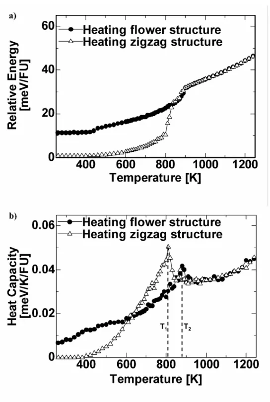
Figure 3-7a shows the thermally averaged energy as a function of increasing temperature in Monte Carlo calculations starting from either a zigzag structure or a flower structure. Even though the flower structure has higher energy at low temperature, it does not transform to the zigzag configuration, indicating that the flower configuration is metastable. In addition, low temperature Monte Carlo calculations reveal that the energy of the partially disordered flower structure (about 10 meV/FU) is significantly lower than the energy of the perfect flower structure (about 26 meV/FU). This indicates that some change takes place in the structure with essentially no kinetic barrier. The driving force of such a change will be discussed later in section 3.5.1. Monte Carlo simulations show that the zigzag structure undergoes a phase transition close to T1 ~

810K, but above this temperature its energy is equal to that of the flower structure. This is indicative of the two initial phases becoming the same phase. Furthermore, an additional phase transition occurs is found at T2 ~ 870K in both sets of calculations.

Figure 3-7b shows the thermally averaged heat capacity from the calculations. This heat capacity only includes the effect of configurational entropy. The result of the zigzag structure simulation show two heat capacity peaks at T1 and T2, which are

(50)

capacity peak in the simulation starting from the flower structure only shows a single peak at T2.

Figure 3-8 shows the Li/Ni disorder, measured as the concentration of Ni in the Li layer and averaged over 50 snapshots of structures at each temperature. The snapshots of the structures were taken at regular intervals (every 2000 passes) during the sampling calculations. The Li/Ni disorder of the zigzag phase is close to zero at the start of the simulation, however, it increases to 8~9% at the first phase transition at T = T1. Above T

> T1, the Li/Ni disorder amount seems to be independent of the starting configuration of

(51)

Figure 3-7. (a) Monte Carlo energy as a function of temperature. (b) Monte Carlo heat capacity as a function of temperature.

(52)

Figure 3-8. Calculated Li/Ni exchange between the Li and TM layers as a function of temperature.

Figure 3-9 is a snapshot of the structure at 850K, which is just above the first phase transition. Figure 3-9a is a good representation of cation arrangement in the TM layer at this temperature range regardless of the starting configuration. There are well-formed "flower" rings consisting of a Li ion surrounded by six Mn ions, which in turn are surrounded by a larger Ni ring. However, substantial disorder, such as LiMn5Ni

rings, Ni-Mn zigzag domains, and even a few MnNi6 rings are present. The presence of

Li surrounded by five Mn and one Ni (as in a LiMn5Ni ring) was also observed in NMR

(30). The ordering in the TM layer discussed further below seems to correlate clearly with the ionic occupation and ordering in the adjacent Li layers.

(53)

The cation ordering patterns observed in the Monte Carlo simulations shows significant local charge imbalance in structures below T2. When flower patterns exist, as

shown in Figure 3-9a, there is a corresponding 2 × 2 ordering pattern of Ni and Li in the Li layer as seen in Figure 3-9b, making this specific region excess in Ni. Although the Monte Carlo cell as a whole is charge balanced, the Monte Carlo snapshot of the Li layer in Figure 3-9b shows concentration of Ni that is a few percent higher than the average Li/Ni disorder value in Figure 3-8.

Above T2, the Ni present in the Li layer disorders and no longer arranges in 2 × 2

patterns. This can be observed in a snapshot of the structure at 1200K in Figure 3-10. Although the TM layer shown in Figure 3-10a appears completely disordered, the average site occupations correspond to the honeycomb scheme mentioned in section 3.2 (30, 31). Li and Ni positions seem to be uncorrelated in the Li layer as shown in Figure 3-10b.

(54)

Figure 3-9. Monte Carlo snapshot at T = 850K of (a) transition metal-rich layer; (b) Li-rich layer. Legend: black: Mn, white: Ni, gray: Li.

(55)

Figure 3-10. Monte Carlo snapshot at T = 1200K of (a) transition metal-rich layer; (b) Li-rich layer. Legend: black: Mn, white: Ni, gray: Li.

(56)

3.5 Discussion

3.5.1 Driving force for the order-disorder transformation in the flower structure

The Monte Carlo simulation shows the most energetically stable cation ordering in the LiNi0.5Mn0.5O2 system as a function of temperature as well as revealing some of the

physics that drive the ordering. The flower pattern can be considered to be a superstructure of the honeycomb structure. In the flower ordering, Li orders in 2√3 × 2√3 patterns in the TM layer. This pattern can be mapped perfectly onto the α sites of the honeycomb pattern, which has √3 × √3 ordering. The central Li atoms in the flower structure occupy 1/4 of the α sites, with Ni occupying the remaining α sites. Mn ions, which occupy the six sites surrounding Li, are all located on β sites. Hence the transformation from the partially ordered flower structure to honeycomb ordering is an order-order transformation whereby Li and Ni disorder on the α sites. Several physical interactions seem to contribute to the ordering into a flower-like arrangement. First, flower ordering was previously shown (49) to be the electrostatically favored configuration of +1, +2 and +4 cations on a two-dimensional triangular lattice describing the TM layer. However, this alone does not seem to fully capture the energetics of the flower structure. The difference between the GGA and GGA+U computation also helps to elucidate the order mechanism. These results point to NiTM - O - NiLi superexchange

between the Li and TM layers which as driving the honeycomb pattern to further order into the flower arrangement (25). Finally when the spins on the Ni in the TM layer and Li

(57)

layer are aligned antiferromagnetically, the Ni 3d orbitals can each hybridize with the same spatial (but different spin) oxygen 2p orbital and delocalize onto the oxygen. This interaction is consistent with the Goodenough-Kanamori rules (50). We have some evidence that this antiferromagnetic interaction is crucial for the stability of the flower. When Ni spins are forced to be ferromagnetic in GGA calculations the flower structure is not the most stable state (25). Furthermore, flower patterns do not form without Li in the TM layer, or in other words, without including Ni in the Li layer (30). A similar case in which interactions that bridge an oxygen are an important factor in the structural stability is the LiA-O-Ni3+-O-LiB 180-degree interaction in LiNiO2 (51, 52).

As seen in Figure 3-9, the flower pattern is accompanied by a 2 × 2 ordering of Ni in the Li layer. The stability of the 2 × 2 pattern can be rationalized by looking at the flower structure in three dimensions (Figure 3-11a). The top and bottom layers show the flower patterns in the TM layer. There are three sites for each flower unit in the Li layer between the two layers (shown in dark gray) that can have the maximum of four NiTM - O

- NiLi bonds. Occupation of all these sites by Ni results in 2 × 2 ordering of Ni in the Li

layer, as is observed in the Monte Carlo calculations.

The competition between the NiTM - O - NiLi bonding and local charge neutrality

leads to frustration in the flower ordered LiNi0.5Mn0.5O2 system. Complete 2 × 2 ordering

(58)

flower ordered in the TM layer. The solution to these competitive forces seems to be to create somewhat higher Li/Ni disorder than the 8.3% (1/12) of the perfectly ordered flower structure. This additional Li/Ni exchange creates more (less) Ni in the Li (TM) layer and as such increases the number of NiTM - O - NiLi bonds that can be formed. This

is why more Li/Ni disorder is created (about 11%) in the Monte Carlo simulations as soon as the temperature is above 0K (Figure 3-8). However, increasing Li/Ni exchange leads to more Li in the TM layer other than the core site of the flower. The Li in sites other than the core site have higher site energy, as they are only coordinated by three or four Mn. Therefore, a Li/Ni exchange of 8 ~ 11 % is observed as a balance of creating favorable NiTM - O - NiLi bonds and unfavorable Li sites in the TM layer. This may also

explain why the Li/Ni disorder decreases with temperature: As the flower structure partially disorders, the frustration between the local charge balance and the NiTM - O -

NiLi bonding can be more easily resolved and requires less additional Li/Ni exchange.

Note in particular how the Li/Ni disorder rapidly decreases in our simulation as the partially disordered flower further disorders into the honeycomb structure at about 620oC (see Figure 3-8).

3.5.2 Partially disordered flower structure

One way to understand the partially disordered flower structure is to look at the structure in both the layered R-3m and the spinel Fd-3m space group settings. In

(59)

LT-LiCoO2, an example of a lithiated spinel-like material, Li occupies 16c sites and Co

occupies 16d sites (13). The relations between the flower structure in the layered and spinel space group settings are similar and depicted in Figure 3-11. Figure 3-11b shows the layered flower structure, but with the sites marked in the spinel setting: the Li layer is composed of 75% 16c sites and 25% 16d sites, and the TM layer is composed of 25% 16c sites and 75% 16d sites. The Ni sites in the Li layer that are likely to create more NiTM -

O - NiLi superexchange bonds are labeled as Li/Ni sites in Figure 3-11a. Note that these

Li/Ni sites correspond to the Li layer 16d sites in Figure 3-11b. The 16c sites in the Li layer are unlikely to contain Ni because these sites do not have the maximum possible number of NiTM - O - NiLi superexchange bonds when the TM layer has a perfect flower

ordering. The 16c sites in the TM layer (top and bottom layers of Figure 3-11b) correspond to the “core” of the flower (the site surrounded by a Mn ring) and the six “corners” of the flower. Each corner is simultaneously a corner of three flower motifs, so there are two corner sites for each core site. The core is Li and the corners are Ni in the perfect flower structure shown in Figure 3-11c. This means that about 2/3 (66.7%) of the 16c sites in the TM layer, which amount to 25% of all 16c sites, are occupied by Ni. Therefore, Ni occupies 1/6 (16.7%) of the total 16c sites in the spinel setting of the flower model because there is no Ni in the 16c sites of the Li layer. On the other hand, Li occupies 2/3 of the 16d sites in the Li layer in the flower structure. In fact, full occupation of all 16d sites in the Li layer by Ni can happen with relatively low energy penalty if the additional Li created in the TM layer only occupies the 16d sites in the TM layer (“edge”

(60)

sites). This exchange leads to the extreme case of a partially disordered flower structure as shown in Figure 3-11d: an ordered structure with all Li/Ni sites (16d) in the Li layer occupied by Ni. In the TM layer, Li occupies some flower “edge” sites (16d), maintaining charge balance of the system as a whole. This configuration has lower energy than the perfect flower structure in GGA+U calculations, but still higher energy than the zigzag structure due to unfavorable Li site occupation in the TM layer. Interestingly, the Li occupancy on the TM-rich 16d sites, or the Ni occupancy on the Li-rich 16c sites is 1/6, although in this scenario, the Li/Ni disorder has increased from 8.3% to 25%. It can be clearly seen that the partially disordered flower structure has the characteristics of both layered (with 3a/3b disorder) and spinel (with 16c/16d disorder) features. One example of such case is in the LiNi0.5Mn0.5O2 sample annealed at 600oC by Lu et al (13). Rietveld

refinement showed 16.1% Li/Ni disorder between the Li and TM layers in the layered setting, and 17.4% Li/Ni disorder between Li-rich 16c sites and TM-rich 16d sites in the spinel setting (13).

(61)

Figure 3-11. (a) Flower structure with emphasis on interaction across layers. Of the 12 sites in the Li layer per flower unit, there are three sites that have four Ni-Ni second nearest neighbors. The Ni in the Li layer prefers these sites. Legend: black: Mn, white: Ni, light gray: Li, dark gray: Li/Ni sites. (b) The flower unit viewed in the spinel setting. Legend: light gray: Li-rich 16c sites, dark gray: Li-poor 16d sites. (c) Perfect flower structure. (d) Partially disordered flower structure with lower first principles energy than the flower shown in (c). Legend: black: Mn, white: Ni, gray: Li.

(62)

3.5.3 Phase transitions

As seen in Figures 3-7 and 3-8, the Monte Carlo simulation clearly shows that upon heating the zigzag structure, at a certain critical temperature (T1) a phase transition

occurs to the flower phase. The perfect flower structure must have achieved higher entropy than the zigzag structure at T1 because it has higher energy at 0K. The entropy

difference can be rationalized through the excitations available for both phases. The zigzag phase has fewer low-energy excitation states than the flower phase. The excitations observed in snapshots of the Monte Carlo simulation from the zigzag phase are simple exchanges of Li and Ni between the Li and TM layers. However, Li in the TM layer prefers to be surrounded by all Mn, which is not possible when it occupies a Ni position in the zigzag structure. Breaking the zigzag ordering in the TM layer requires relocation of a large number of cations, which is difficult in Monte Carlo simulations at low temperatures. Therefore, putting Li in the TM layer of the zigzag phase carries a heavy energy penalty since Li can at best be surrounded by four Mn. In contrast, the majority of Li are surrounded by six Mn in the flower phase. In addition, the flower patterns can form and disintegrate relatively easily in the honeycomb framework in the TM layer (30, 31). The honeycomb ordering guarantees that no Li-Li nearest-neighbor pairs occur in the TM layer, which would come with a strong electrostatic energy penalty. Also the flower phase becomes stable above a certain temperature where the zigzag phase cannot tolerate much Li/Ni disorder because of the difference in excitations.

Computational structure analysis of multicomponent oxides

Computational Structure Analysis of Multicomponent Oxides

by

Yoyo Hinuma

Author . . .

Department of Materials Science and Engineering

April 10, 2008

Certified by . . .

Gerbrand Ceder

R. P. Simmons Professor of Materials Science and Engineering

Thesis Supervisor

Accepted by . . .

Samuel Miller Allen

POSCO Professor of Physical Metallurgy

Computational Structure Analysis of Multicomponent Oxides

by

Yoyo Hinuma

Abstract

Acknowledgments

Contents

Chapter 1 Introduction

Chapter 2 Computational phase diagram generation

∑

∑

∑

( )

(

)

∑

( )

( )

∑

(

(

)

)

∑

(

)

(

)

(

)

(

)

(

)

∑

∑

(

)

(

)

(

)

∫

( )

(

)

(

)

∑

∑

(

)

(

)

(

)

∫

( )

( ) ( ) (

)

∑

∫

Chapter 3 The lithium battery material Li

Ni

Mn

O

_∑

_∑

_∫

₍

₎