Computational and theoretical study of electron phase-space holes in kinetic plasma: kinematics, stability and ion coupling

Computational and theoretical study of electron

phase-space holes in kinetic plasma: kinematics,

stability and ion coupling

by

Chuteng Zhou

Ing´enieur dipl^om´e, CentraleSup´elec (2013)

M.Sc., Columbia University (2013)

Submitted to the Department of Nuclear Science and Engineering

in partial fulfillment of the requirements for the degree of

Doctor of Philosophy in Applied Plasma Physics

at the

MASSACHUSETTS INSTITUTE OF TECHNOLOGY

February 2018

c

○ Massachusetts Institute of Technology 2018. All rights reserved.

Author . . . .

Department of Nuclear Science and Engineering

February 5, 2018

Certified by . . . .

Ian H. Hutchinson

Professor of Nuclear Science and Engineering

Thesis Supervisor

Certified by . . . .

Nuno F. Loureiro

Associate Professor of Nuclear Science and Engineering

Associate Professor of Physics

Thesis Reader

Accepted by. . . .

Ju Li

Battelle Energy Alliance Professor of Nuclear Science and Engineering

Professor of Materials Science and Engineering

Chairman, Department Committee on Graduate Theses

Computational and theoretical study of electron phase-space

holes in kinetic plasma: kinematics, stability and ion coupling

by

Chuteng Zhou

Submitted to the Department of Nuclear Science and Engineering on February 5, 2018, in partial fulfillment of the

requirements for the degree of

Doctor of Philosophy in Applied Plasma Physics

Abstract

In this thesis, a comprehensive study of Bernstein-Greene-Kruskal (BGK) mode electron holes in a collisionless plasma where strong kinetic effects are important is presented. Kinematic theory based on momentum conservation is derived treating the electron hole as a composite object to study the dynamics of electron holes. A novel 1-D Particle-In-Cell simulation code that can self-consistently track the electron hole motion has been developed for the purpose of this thesis work. Quantitative agreement is achieved between analytic theory and simulation observations. The thesis reports a new kind of instability for electron holes. Slow electron holes traveling slower than a few times the cold ion sound speed in the ion frame are observed to be unstable to the oscillatory velocity instability. A complete theoretical treatment for the instability is presented in this thesis. Numerical simulations yield quantitative agreement with the analytic theory in instability thresholds, frequencies and partially in instability growth rates. It is further shown that an electron hole can form a stable Coupled Hole Soliton (CHS) pair with an ion-acoustic soliton. A stable CHS travels slightly faster than the ion-acoustic velocity in the ion frame and is separated from a typical BGK mode electron hole in the velocity range by a gap, which is set by the oscillatory velocity instability. Transition between the two states is possible in both directions. A CHS exhibits a soliton-like behavior. The thesis sheds light on solving the ambiguity between an electron hole and a soliton. This thesis work also has important implications for interpreting space probes observations.

Thesis Supervisor: Ian H. Hutchinson

Title: Professor of Nuclear Science and Engineering Thesis Reader: Nuno F. Loureiro

Title: Associate Professor of Nuclear Science and Engineering Associate Professor of Physics

Acknowledgments

I remember reading the PhD Grind by Philip Guo before starting my PhD to prepare for this formidable journey. I thought to myself, what kind of grind will my PhD be? Now here I am, almost five years later, at the edge of finishing my PhD; when I look back, though there have been ups and downs, my overall experience as a PhD student at MIT has been quite enjoyable. I would like to acknowledge the people who have made my PhD experience a memorable intellectual journey.

First, I would like to acknowledge my research adviser Prof. Ian Hutchinson. Ian has always advised and guided me with his extensive knowledge, wisdom and sheer profes-sionalism throughout my PhD. Ian is a great teacher, he approaches the PhD education as an “apprenticeship” (his own word). He provided valuable hands-on training while I was beginning my PhD and then gave me the freedom to perform my own research once I became independent enough. It is a pleasure to collaborate with Ian. He always reports his own progress at our weekly meeting, it is a boost to my own productivity as Ian is constantly challenging me with new ideas. Ian advises with humility, he treats me as an equal and always values what I have to say. Ian holds our scientific work to the highest standards and does not stand the slightest sloppiness. I feel extremely privileged to have Ian as my adviser and mentor during my PhD.

I would like to thank Chris Haakonsen. Chris was a senior PhD student in the group when I first joined. We worked together and shared office. Chris provided guidance and helped with many difficulties I encountered as a junior PhD student. His master-level computer science skills were extremely helpful. His work is the foundation of many results I accomplished in this thesis. Chris is a very sharp individual, I benefited a lot from our discussions about both work and life.

I would like to acknowledge the members of my thesis committee, Prof. Nuno Loureiro and Prof. Jeff Freidberg for the valuable advice on my research and continuous support during my PhD. I would like to acknowledge many other good teachers I have had at MIT, Prof. Anne White, Prof. Dennis Whyte, Prof. Miklos Porkolab, Dr. Paul Bonoli and Prof. Mehran Kardar for their exciting lectures and the key knowledge I received to carry

out my PhD work. I would like to acknowledge Dr. John Wright for his help with Loki and engaging computing clusters on which the thesis work is carried out. I would like to thank Brandon Savage and Lee Berkowitz for their help with IT problems. I would like to acknowledge Valerie Censabella, Jessica Coco, Brandy Baker, Heather Barry and Peter Brenton for the daily administrative support. I would like to acknowledge Dr. Marina Dang for helping me to improve my communication skills.

I would like to acknowledge teachers and supervisors I have had prior to MIT who got me interested in plasma physics: Prof. Mike Mauel, Dr. ¨Ozg¨ur G¨urcan, Prof. Francesco Volpe, Prof. Andrew Cole. I would like to thank Dr. David Malaspina for the helpful discussions and educating me about space physics.

I am grateful to the sponsors of my PhD and research work: Mr. Ray Rothrock through the Rothrock fellowship, US Department of Energy and National Science Foundation through Grant DE-SC0010491, National Aeronautics and Space Administration through Grant NNX16AG82G.

I would like to acknowledge Lulu Li, Will Boyd, Bob Mumgaard, Zach Hartwig, Ted Golfinopoulos, Ian Faust, John Walk, Mark Chilenski, Harold Barnard and Brandon Sorbom for their help and advice during my PhD. I would like to acknowledge the fellow graduate students at PSFC and NSE: Silvia Espinosa, Juan Ruiz Ruiz, Leigh Ann Kesler, Adam Kuang, Alex Tinguely, Alex Creely, Norman Cao, Libby Tolman, Sameer Abraham, Pablo Rodriguez-Fernandez, Haoran Xu, Xueying Lu, Pablo Ducru, Cong Su, Lun Yu, Yang Yang, Akira Sone, Xuejun Huang, Zhaoyuan Liu for being excellent peers and friends.

I would like to acknowledge other friends in the Boston area: Quntao Zhuang, Zheng Li, Jing Wang, Yinan Wang, Zhicheng Yang, Le Wang, Zhuoxuan Li, Hui Wang, Yongbin Sun, Ziwen Liu, Qingyang Wang, Ryan King, Chiwei Yan, Yiwen Zhu, Youzhi Liang, Ziqin Rong, Jiawei Zhou, Yue Guan, Yuxuan Ye, Qiao Zheng, Xiaofeng Yang, Lele Tang, Jieyu Chen, Tong Tong. Thank you so much for your friendship and support. I would like to acknowledge my friends from high school: Cheng Xu, Shihan Tao and Shangjun Zhang for being good friends to me for such a long time and all the happy time and help

you’ve given me during my PhD at MIT.

J’aimerais remercier M. Jean Aristide Cavaill`es, M. Herv´e Riou pour me donner un go^ut pour les sciences physiques. J’aimerais remercier M. Gil Guibert et M. Michel Cognet pour m’enseigner comment penser en math´ematiques et les techniques qui m’ont beaucoup servi pendant ma th`ese. J’aimerais remercier sp´ecialement Bruno et Pascale Seznec pour leur amiti´e et encouragement.

I would like to thank my girlfriend Jiahua for her love and support that is most dear to my heart. I am deeply indebted to my parents for their love and care thoughout my entire life. They have always supported my choice and encouraged me to pursue my dreams. 负笈离家十数载, 父母养育恩难忘.

Contents

1 Background 23

I Modeling plasma dynamics: kinetic equations . . . 24

II Computer simulation tools for kinetic plasma . . . 30

II.1 Vlasov code . . . 30

II.2 Particle-In-Cell (PIC) code . . . 31

III BGK mode electron holes . . . 34

III.1 Integral equation approach . . . 36

III.2 Differential equation approach . . . 38

III.3 Observational features of electron holes . . . 40

III.4 Electron holes in higher dimensions . . . 42

III.5 Electron holes in plasma wake of an object . . . 43

IV Other nonlinear solitary wave phenomena in plasma . . . 45

IV.1 Ion-acoustic soliton and the Korteweg-de Vries equation . . . 46

IV.2 Schamel’s modified Korteweg-de Vries equation with resonant elec-trons . . . 49

V Thesis motivation and outline . . . 50

2 Electron hole kinematics deduced from momentum conservation 53 I Ion momentum rate of change . . . 54

I.1 Momentum change due to hole acceleration . . . 55

I.2 Momentum change due to hole growth . . . 59

III Acceleration caused by hole growth . . . 65

IV Electron hole momentum coupling to ions by hole pushing and pulling . . . 66

V Conclusions . . . 68

3 Hole tracking Particle-In-Cell simulation 71 I Hole tracking simulation . . . 72

II Initial transient to steady state . . . 77

III Hole pushing and pulling . . . 90

IV Summary . . . 96

4 Plasma electron hole velocity oscillatory instability 99 I PIC observation of the instability . . . 101

II Hole velocity stability deduced from kinematics . . . 105

II.1 Frequency response of the momentum rate of change . . . 105

II.2 Counter-streaming ions . . . 118

II.3 Linear growth rate . . . 119

II.4 Finite ion temperature . . . 122

III Eigenmode ansatz derived from linearized Vlasov-Poisson system . . . 123

IV Discussion . . . 129

V Conclusion . . . 132

5 Slow electron hole coupled to an ion-acoustic soliton 133 I Coupling an electron phase space hole to an IAS . . . 135

II Collision of Coupled Hole Soliton (CHS) pairs . . . 138

III Velocity gap and transition between two states . . . 143

III.1 Velocity gap between CHS and BGK states . . . 143

III.2 Transition from CHS to BGK by ion Landau damping . . . 146

III.3 Transition from BGK to CHS by hole growth . . . 148

IV Buneman instability and CHS formation . . . 152

V Implications for space observation . . . 154

6 Conclusions and future work 159 I Conclusions . . . 159 II Future directions . . . 161

A Initial electron distribution generated by rejection method 165

B Rate of change of contained ion momentum 167

List of Figures

1-1 Schematic of the leapfrog algorithm. . . 32 1-2 Left: Computing particles with spatial ”cells” in PIC. Right: the processes

involved in advancing one time step in PIC. . . 32 1-3 Formation of electron holes in a 1-D PIC simulation . . . 35 1-4 Top: electrostatic potential 𝜑(𝑥) of an electron hole. Bottom: electron

phase space orbits, the shaded orbits are trapped. . . 37 1-5 (a) Electron velocity distribution at the hole center (b) Electron

phase-space density assuming a Maxwellian background plasma (c) Sagdeev po-tential 𝑉 as a function of 𝜓 − 𝜑 (d) Electrostatic popo-tential profile of the solitary electron hole . . . 39 1-6 Parallel electric field measurement showing electron holes within magnetic

reconnection diffusion region at magnetopause, measured by Cluster satellite 41 1-7 Schematic of a THEMIS mission satellite . . . 42 1-8 Kinetic simulation of the plasma wake behind an unmangetized object . . . 44 1-9 Event density of electron hole encounters around the moon, colors show

the number of events. The contours are iso-density contours for protons showing the shape of lunar wake. Courtesy of David Malaspina. . . 45 2-1 Top: a passing particle exits the hole region with exactly the same velocity

as it enters when the hole has a constant velocity and does not change its shape. Bottom: there is change in passing particle velocity and density thus momentum transfer when the hole is accelerating or changing its shape. 55 2-2 Plot of ℎ(𝜒) compared with its asymptotic approximations. . . 65

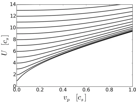
2-3 𝑈 as a function of 𝑣𝑝 obtained by solving Equation (2.44) with 𝑚𝑖/𝑚𝑒 =

1836 and different 𝑈0. . . 67

3-1 Block diagram of hole tracking. 𝜌(𝑥) and 𝜑(𝑥) are charge density and potential in the simulation, 𝑥ℎ and 𝑣ℎ are position and velocity of electron

hole, ˜𝑣ℎis the hole velocity after smoothing is applied, 𝑣𝑏and 𝑎𝑏 are velocity

and acceleration of simulation box. . . 73 3-2 Velocity of an electron hole in two different runs, in the fixed domain run,

the electron hole hits the boundary at 𝜔𝑝𝑒𝑡 = 590 while the hole tracking

run can successfully simulate hole motion for a much longer period of time. Velocity data shown here are smoothed using a low-pass filter of cutoff frequency 0.15 𝜔𝑝𝑒. . . 76

3-3 a) Normalized electron phase space density contours b) Potential, c) Ion density, d) Electron density. Position 𝑥 and velocity 𝑣 are relative to lab frame. The plots shown on the same row are from the same time step in the simulation. . . 79 3-4 Lab frame velocity of electron hole and simulation domain. The plot on

the right is a close-up examination of the initial transient for the same run. Hole velocity is smoothed using a low-pass filter of cutoff frequency 0.15 𝜔𝑝𝑒. 81

3-5 Steady state hole velocity in initial ion rest frame as a function of mass ratio, steady state hole depth and initial hole velocity, solid curves in each plot are obtained from hole momentum conservation theory. . . 83 3-6 Potential and electron density profile for two steady state electron holes

of different depths and speed compared with Schamel’s analytic solution, 𝑒𝜓 = 0.23𝑇𝑒, 𝑣ℎ = 6.9𝑐𝑠 on the left and 𝑒𝜓 = 0.05𝑇𝑒, 𝑣ℎ = 3.8𝑐𝑠 on

the right, simulation results are averaged over 100 time steps to reduce fluctuations. . . 85 3-7 Electron distribution on constant energy ℰ orbit in hole frame, 𝑒𝜓 =

0.23𝑇𝑒, 𝑣ℎ = 6.9𝑐𝑠. Dashed line is Schamel’s solution for an electron hole

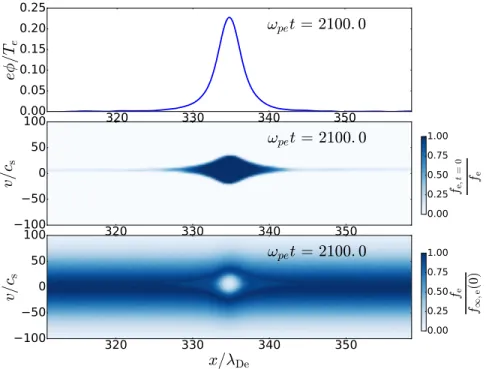
3-8 The hole potential (top panel), the relative phase space density of initial electrons (middle panel) and the normalized electron phase space density (bottom panel) at time 𝜔𝑝𝑒𝑡 = 2100, the hole has a lab frame velocity of

6.9𝑐𝑠, 𝑥 and 𝑣 are relative to lab frame. . . 88

3-9 Coalescence of electron holes of different size in our simulation, a shallow hole is followed by a much deeper one and they eventually partly coalesce. A piece of the shallower hole is sprayed out. This run is performed with 𝑈0 = 7𝑐𝑠,𝑚𝑖/𝑚𝑒 = 1836 and the deeper hole at the center of simulation

domain has a depth of 𝑒𝜓 = 0.23𝑇𝑒, the shallower hole has a depth of

𝑒𝜓 = 0.03𝑇𝑒. . . 89

3-10 Hole velocity response to artificial ion acceleration, 𝑇𝑒/𝑇𝑖 = 20 , 𝑒𝜓 =

0.1𝑇𝑒. Solid line is the “pushing” run and dashed line is the “pulling” run.

Dashed dot line is a reference run where no artificial acceleration is applied. 91 3-11 Hole pushing and pulling runs for holes of different depths using two

dif-ferent mass ratios. The value of 𝜓 is the average value during acceleration. 𝑇𝑒/𝑇𝑖 = 20 , 𝑁𝑖 = 𝑁𝑒 = 2.56 × 107. . . 93

3-12 Illustration of reversibility and hysteresis in pushing and pulling. (a) Push-ing, pulling and no ion acceleration runs showing spontaneous hole velocity decay and hysteresis. (b) The same runs as (a) with eight times as many particles, the spontaneous velocity decay and hysteresis are reduced by us-ing more particles. The number of computation cells is 1000 in these runs and the domain length is 48𝜆De across. 𝑇𝑒/𝑇𝑖 = 20 , 𝑒𝜓 = 0.1𝑇𝑒. . . 95

4-1 The hole potential (first row) and the ion density (second row) before (left) and after (right) the instability growth. Bottom left panel shows the EH velocity in the ion frame and the bottom right panel shows the ion density perturbations due to the EH and the instability. The bulk electrons are Maxwellian at rest in the laboratory frame and 𝑇𝑒/𝑇𝑖 = 20. . . 103

4-2 The hole potential (first row) and the ion density (second row) before (left) and after (right) the instability growth in a plasma with counter-streaming ions. Bottom left panel shows the EH velocity and the bottom right panel shows the ion distribution function with counter-streaming Maxwellians. The ion streams have an average velocity of ±6.7𝑐𝑠 and 𝑇𝑖 = 𝑇𝑒. The bulk

electrons are Maxwellian at rest in the lab frame. . . 104 4-3 Schematic of a steady-state EH with the associated phase-space structure

and the ion response. Top: EH potential, middle: electron phase space orbits, the trapped orbits are shaded. Bottom: the steady-state ion velocity 𝑣0 and density 𝑛0 in the hole frame. . . 106

4-4 (a): ˙𝑃𝑖/ ˙𝑃𝑒evaluated on the real axis for 𝜑 = 0.23 sech4(𝑥/4) , 𝑚𝑖/𝑚𝑒 = 1836

and three different hole speeds. ˙𝑃𝑖/ ˙𝑃𝑒(𝜔) + 1 = 0 has two unstable zeros

when |𝑈 | < 𝑈𝑐= 4.6𝑐𝑠 here. (b): 𝐹 (𝜔/𝑈 ) function defined in Eqn. (4.24)

evaluated for 𝜔 on the real axis using ˜𝜑(𝑥) = sech4(𝑥/4). 𝐹 contour is invariant for different hole velocity 𝑈 . . . 113 4-5 The critical values of hole speed in the ion frame below which the instability

occurs for different sized EHs and two different mass ratios. The theoretical stability boundaries (𝛾 = 0) and the 𝛾 = 0.1 growth rate boundaries for Schamel type of EHs 𝜑(𝑥) = 𝜓 sech4(𝑥/4) are plotted as reference lines. The observational data point and the numerical calculation of the same 𝜓 correspond to the same run. The ion reflection limit is much lower than the instability threshold, hence our approximation 𝑈2 _{≫ 2𝜓 is well satisfied.}

All the PIC runs have 𝑇𝑒/𝑇𝑖 = 20. . . 116

4-6 The oscillations seen in our simulation are Fourier analyzed to extract its main frequency for the first few periods of unstable oscillations. The uncertainty in the theoretically predicted frequency due to the uncertainty of 𝑈𝑐 used in Eqn. (4.36) is shown by the gray uncertainty bands. Notice

that the unstable oscillation frequency is in general a few times the ion plasma frequency. . . 117

4-7 Instability growth rate 𝛾 as a function of Δ𝑈 . The linear relation repre-sents Eqn. (4.46) for fixed hole shape. Its uncertainty bands represent the small variation of shape from one run to another, giving uncertainty in the comparison. The triangles are obtained from solving numerically the full eigenmode equation ˙𝑃𝑖/ ˙𝑃𝑒+ 1 = 0 using the PIC potential output. Circles

are the growth rate observed in PIC runs. . . 121 4-8 Finite ion temperature effect on the 𝐹 contour for a Schamel type of EH.

The contour shape is approximately preserved while its size grows with a larger 𝑇𝑖. . . 124

4-9 Phase-space density of trapped electrons in our hole-tracking PIC simula-tion before and after the instability onset. The EH is broken into smaller pieces by this instability. . . 131 5-1 a) Normalized electron phase space density contours b) Potential, c) Ion

density, d) Electron density. The plots shown on the same row are from the same time step in the simulation. . . 136 5-2 Head-on collision of two CHSs, the left CHS travels at 1.5𝑐𝑠 and the right

CHS travels at −1.5𝑐𝑠. Both electrostatic potential (solid line) and ion

density (dashed line) are shown in this plot. . . 140 5-3 Head-on collision of similar-sized electron phase space holes with

compa-rable velocity difference as in Figure 5-2 without ion-acoustic solitons at-tached, the left electron hole travels at 1.2𝑐𝑠; the right electron hole travels

at −2𝑐𝑠 and the merged hole travels at −1.2𝑐𝑠. The electrostatic potential

is shown in solid line. . . 141 5-4 Left: electron phase space density during a CHS head-on collision. Right:

ion density during the collision at the same time slices. . . 142 5-5 Pure electron holes not coupled to ion-acoustic solitons merging during a

head-on collision. . . 143 5-6 Velocity and amplitude of the solitary waves observed in our PIC simulation

5-7 Long-term evolution of a CHS in a plasma where 𝑇𝑒/𝑇𝑖 = 5 shows

insta-bility while the ion density compressional pulse is damped away by ion Landau damping. The electrostatic potential is shown in solid line and the ion density is shown in dashed line. The last row shows the final free electron hole released from the CHS by instability. Hole tracking simu-lation is used to track the long-term behavior of this solitary wave. The 𝑥-coordinate is with respect to the lab frame. . . 147 5-8 Velocity of the solitary wave during and after the instability showing the

transition, the velocity is measured by hole tracking algorithm described in Chapter 3. A low-pass filter of cutoff frequency 0.03𝜔𝑝𝑒 is applied to the

velocity time series to eliminate high-frequency noise. . . 148 5-9 Electrostatic potential and ion density during the growing density

simula-tion. Background density growth starts at 𝜔𝑝𝑒𝑡 = 30 and ends at 𝜔𝑝𝑒𝑡 = 1200.150

5-10 Velocity of the solitary wave during the rising density simulation. The wave converges to a stable CHS state. The same low-pass filtering is applied as in Figure 5-8. . . 151 5-11 Top: ion phase space of the CHS at 𝜔𝑝𝑒𝑡 = 3330. Bottom: electron phase

space of the CHS at 𝜔𝑝𝑒𝑡 = 3330. . . 151

5-12 Top: Buneman instability simulation with cold ions shows formation of CHS-like structures, traveling slightly above 1𝑐𝑠 in the ion frame. Bottom:

Buneman instability simulation with a hotter ion population only shows formation of BGK electron holes, traveling between 4𝑐𝑠 and 5𝑐𝑠 in the ion

frame, above the stability threshold velocity. . . 153 5-13 The velocity-amplitude parameter plane. The velocity is normalized to cold

ion sound speed and the amplitude is normalized to electron temperature. The BGK mode free electron holes are separated from the CHSs by the shaded region, which represents the oscillatory velocity instability. . . 155

5-14 The observational data from Cluster spacecraft are plotted in the velocity-amplitude parameter plane. The ones with speed close to 𝑐𝑠 are referred

to as the “Slow Electrostatic Solitary Waves”. These data are published in references [92, 99]. . . 156 6-1 Transverse instability of a two-dimensional electron hole. The magnetic

field is along axis 1. The top panel (a) shows the simulation at 𝜔𝑝𝑒𝑡 = 204,

the bottom panel (b) shows the simulation at 𝜔𝑝𝑒𝑡 = 628. Courtesy of I.

Nomenclature

𝜖0 Vacuum permittivity

𝜇0 Vacuum permeability

𝜔𝑏 Bounce frequency of deeply trapped electrons: √︀𝑒𝜓/𝑚𝑒/𝐿

Ω𝑒 Electron cyclotron frequency:

√︂ 𝑒𝐵 𝑚𝑒

𝜔𝑝𝑒 Electron plasma frequency:

√︂ 𝑛𝑒2

𝜖0𝑚𝑒

𝜑 Electrostatic potential 𝜓 The maximum of 𝜑

˜

𝜑 Normalized electrostatic potential: 𝜑/𝜓 𝑐 Speed of light in vacuum

𝑐𝑠 Cold ion sound speed:

√︂ 𝑇𝑒

𝑚𝑖

ℎ Planck constant

𝐿 Spatial dimension of an electron hole parallel to the magnetic field direction 𝑀 Mach number of a velocity normalized to 𝑐𝑠

𝑁 Number of particles

𝑈 Electron hole velocity in the plasma or the ion frame 𝑉 Volume

𝑣th,e Electron thermal speed:

√︂ 𝑇𝑒

𝑚𝑒

𝑣th,i Ion thermal speed:

√︂ 𝑇𝑖

𝑚𝑖

𝑣ℎ Electron hole velocity in the rest frame of background electrons

𝑣𝑑,𝑒 Drift velocity of bulk electrons in the ion frame

𝑣𝑝,𝑒 Marginal passing velocity for electrons:

√︂ 𝑒𝜓 𝑚𝑒

𝑣𝑝,𝑖 Marginal passing velocity for ions:

√︂ 𝑒𝜓 𝑚𝑖

Chapter 1

Background

Plasma is the ionized matter that makes up more than 99% [1] of the visible matter in our universe. Understanding plasma is thus crucial for the understanding of our uni-verse. Plasma physics is the branch of physics that studies this particular state of matter. Research in plasma physics is also driven by the numerous industrial applications. To name a few, the entire modern semiconductor industry is made possible by high precision plasma etching tools [2]. Plasma is also widely used in surface treatment [3] and indus-trial pollution control [4]. Plasma technology based ion thrusters provide a much higher specific impulse alternative to the traditional chemical rockets [5], potentially powering spacecrafts for deep space travel. Plasma wake-field acceleration [6] is expected to create highly-efficient compact particle accelerator in the future. The most sought-after appli-cation of plasma physics is nuclear fusion [7], the holy grail of all forms of energy. The extreme physical conditions required by nuclear fusion necessarily demands dealing with matter in form of plasma. Despite great scientific and technological hurdles, mankind has been pursuing controlled nuclear fusion relentlessly for decades. The enormous amount of resources put into fusion research greatly advanced the state of plasma physics in the last decades.

The Sun is the fusion reactor at the center of the Solar System. Fusion energy from the Sun radiates out both in form of electromagnetic radiations and particle fluxes [1]. The extremely hot particles coming out of the solar atmosphere are in form of plasma and

are known as solar wind [1]. The solar wind is blown out into the entire Solar System, forming a giant plasma bubble known as the heliosphere [1]. Near Earth, the dynamics of plasma is strongly controlled by Earth’s magnetic field. This region of space is known as Earth’s magnetosphere [1]. Earth’s magnetosphere is partially responsible for blocking highly energetic harmful cosmic rays [8] from reaching the surface of Earth. Closer to Earth, the upper Earth atmosphere is ionized by radiation and forms the inner edge of the magnetosphere. This plasma layer is known as ionosphere [9]. The ionosphere is very important for telecommunication on Earth as it influences the propagation of electromag-netic waves [9]. Most man-made satellites travel in the magnetosphere, ionosphere or the heliosphere. The study of these plasma bodies near Earth and in the Solar System is a particular branch of physics known as space physics [1]. In addition to better under-standing space environment, space physics is particularly important for the operation of satellites and manned flight in space [10]. Many spacecraft have been launched in the last few decades to provide in situ measurements for space physics research. This thesis is at the intersection of plasma physics and space physics.

I

Modeling plasma dynamics: kinetic equations

A plasma consists of charged particles. The force felt by a charged particle traveling in the electromagnetic field is the Lorentz force

F= 𝑞 (E + v × B) . (1.1)

We adopt SI units throughout this thesis. When the particle velocity is much slower than the speed of light and the inter-particle distance is much bigger than the thermal de Broglie wavelength, namely,

𝑣 ≪ 𝑐 , √ ℎ 2𝜋𝑚𝑇 ≪ (︂ 𝑉 𝑁 )︂1₃ , (1.2)

the plasma is in the classical limit where relativistic and quantum mechanics effects are negligible [11]. The plasma bodies studied in space physics are mostly in this classical limit [11]. A classical plasma can be described by solving simultaneously Newton’s equations of motion and Maxwell’s equations for the electromagnetic field. A plasma is a collection of particles interacting with one another through self-consistent electromagnetic interactions, the density of a plasma ranges from for example 106 _{particles per cubic meter in solar}

wind to 1021 _{particles per cubic meter in a fusion reactor and higher still within stars}

[7]. In principle, the equations of motion are solved for each particle simultaneously while the Maxwell’s equation takes into account more macroscopic quantities such as charge and current density. A mathematical way to describe this particle ensemble needs to be introduced to make the problem more tractable. A complete description of a plasma can be specified given the coordinate x𝑖(𝑡) and velocity v𝑖(𝑡) of each particle 𝑖 of species 𝛼.

We define a function 𝐹 𝐹𝛼(x, v, 𝑡) = 𝑁𝛼 ∑︁ 𝑖=1 𝛿(x − x𝑖)𝛿(v − v𝑖), (1.3)

where subscript 𝛼 designates particle species. We can thus write down the charge density and current density in the following forms

𝜌 =∑︁ 𝛼 𝑞𝛼 ∫︁ 𝐹𝛼(x, v, 𝑡) 𝑑v, (1.4) 𝑗 =∑︁ 𝛼 𝑞𝛼 ∫︁ v𝐹𝛼(x, v, 𝑡) 𝑑v. (1.5)

The electric and magnetic fields due to the plasma particles are given by ∇ · E = ∑︁ 𝛼 𝑞𝛼 ∫︁ 𝐹𝛼(x, v, 𝑡) 𝑑v 𝜖0 , (1.6) ∇ · B = 0, (1.7) ∇ × E = −𝜕B 𝜕𝑡, (1.8) ∇ × B = 𝜇0( ∑︁ 𝛼 𝑞𝛼 ∫︁ v𝐹𝛼(x, v, 𝑡) 𝑑v + 𝜖0 𝜕E 𝜕𝑡). (1.9)

From the equation of motion and the conservation of particles, we get an equation that governs the evolution of 𝐹𝛼(x, v, 𝑡)

𝜕𝐹𝛼(x, v, 𝑡) 𝜕𝑡 + v · 𝜕𝐹𝛼(x, v, 𝑡) 𝜕x + 𝑞𝛼 𝑚𝛼 (E + v × B) · 𝜕𝐹𝛼(x, v, 𝑡) 𝜕v = 0. (1.10)

Equation (1.10) is the Klimontovich-Dupree equation [12] of plasma dynamics. However, it is not particularly useful as 𝐹𝛼(x, v, 𝑡) is composed of Dirac delta functions, which are

distributions in the strict mathematical sense instead of being a classically differentiable statistical function. The common way to remedy this is to introduce a differentiable and non-negative phase-space probability function 𝜌𝛼,𝑁(x1, ..., x𝑁; v1, ..., v𝑁, 𝑡) defined as

the density of probability at a time 𝑡 to find particles of species 𝛼 to have coordinates and velocities of the values x1, x2, ..., x𝑁; v1, v2, ..., v𝑁. 𝜌𝛼,𝑁 is a probability density so its

integral over the entire 6𝑁 -dimensional phase space is 1. The total amount of information contained in this 6𝑁 -dimensional phase space is much more than what we need to describe the bulk properties of a plasma and 𝜌𝛼,𝑁 as a function of 6𝑁 + 1 arguments is difficult

to deal with. We need to simplify this problem even more at the expense of losing some unimportant detailed information. We introduce a one particle density function 𝑓𝛼,1given

by

𝑓𝛼,1(x, v, 𝑡) = ⟨𝐹𝛼(x, v, 𝑡)⟩ (1.11)

= 𝑁𝛼

∫︁

𝑓𝛼,1(x, v, 𝑡) represents the expectation value of finding any of the 𝑁 particles of species 𝛼

at coordinate x and velocity v. We have assumed that the probability density function is symmetric with respect to permuting the particles. In a similar way, we can define the general 𝑠-particle density function 𝑓𝛼,𝑠 as the follow

𝑓𝛼,𝑠(x1, v1, ..., x𝑠, v𝑠, 𝑡) = 𝑁 ! (𝑁 − 𝑠)! ∫︁ 𝑁 ∏︁ 𝑖=𝑠+1 𝑑x𝑖𝑑v𝑖𝜌𝛼,𝑁. (1.12)

By averaging the Klimontovich-Dupree equation using the probability density function, one can transform [12] the original equation (1.10) into an infinite chain of statistical equations involving the 𝑠-particle density functions 𝑓𝛼,𝑠 defined above, with 𝑓𝛼,𝑠 being

involved in the equation of 𝑓𝛼,𝑠−1. It is very difficult to solve this infinite chain of equations.

However, it is possible to take advantage of the statistical property of the system to terminate the chain at the first few orders and give an approximation for the higher order terms. In a plasma, the small parameter is often chosen as 𝑔 = 1/𝑛𝜆3

De ≪ 1, the

inverse of the number of particles in the Debye sphere. Debye length 𝜆De = √︀𝜖0𝑇 /𝑛𝑞2

is the characteristic electric field shielding distance in a plasma. A plasma satisfying this property is said to be weakly-coupled or ideal. The plasma studied in space physics and the fusion plasma are typically ideal plasma with 𝑔 < 10−5_{. It can be proved in this case}

that each hierarchy of statistical equation is of order 𝒪(𝑔) smaller than the previous one [12, 13]. To the lowest order, the kinetic equation for the plasma can be written as

(︂ 𝜕 𝜕𝑡+ v · ∇x+ 𝑞𝛼 𝑚𝛼 (E + v × B) · ∇v )︂ 𝑓𝛼(x, v, 𝑡) = 0, (1.13)

where we have used interchangeably 𝑓𝛼(x, v, 𝑡) and 𝑓𝛼,1(x, v, 𝑡) to simplify the notation.

Equation (1.13) is called the Vlasov equation or the collisionless Boltzmann equation. Coupled with Maxwell’s equations, it describes the behavior of the plasma on a time scale shorter than the typical collision time scale: 𝜏collective≪ 𝜏collision. The Vlasov equation

regime: ⎧ ⎪ ⎪ ⎪ ⎪ ⎪ ⎪ ⎪ ⎪ ⎪ ⎪ ⎪ ⎪ ⎪ ⎪ ⎪ ⎪ ⎨ ⎪ ⎪ ⎪ ⎪ ⎪ ⎪ ⎪ ⎪ ⎪ ⎪ ⎪ ⎪ ⎪ ⎪ ⎪ ⎪ ⎩ (︂ 𝜕 𝜕𝑡 + v · ∇x+ 𝑞𝛼 𝑚𝛼 (E + v × B) · ∇v )︂ 𝑓𝛼(x, v, 𝑡) = 0, ∇ · E = ∑︁ 𝛼 𝑞𝛼 ∫︁ 𝑓𝛼(x, v, 𝑡) 𝑑v 𝜖0 , ∇ · B = 0, ∇ × E = −𝜕B 𝜕𝑡, ∇ × B = 𝜇0( ∑︁ 𝛼 𝑞𝛼 ∫︁ v𝑓𝛼(x, v, 𝑡) 𝑑v + 𝜖0 𝜕E 𝜕𝑡). (1.14)

This approximation corresponds to the mean field approach in statistical mechanics [13], modeling plasma particle dynamics with self-consistent long-range electromagnetic inter-actions. It is well-adapted for the dilute plasma studied in space physics. The mean free path for both the electrons and the ions are bigger than the Earth radius in the magne-tosphere [1]. We are in a highly collisionless regime for the kind of plasma phenomenon we are going to introduce in the next section. The collisional corrections appearing in the higher order kinetic equations are often lumped into a single collision operator 𝐶(𝑓𝛼, 𝑓𝛼)

to be placed at the right hand side of Equation (1.13) instead of 0. This hierarchy of kinetic equations is called the BBGKY hierarchy [13], named after Bogolyubov, Born, Green, Kirkwood and Yvon. For the purpose of this thesis, we are going to focus on the collisionless mean field model.

The equation system (1.14) can be further simplified for an electrostatic plasma. This approximation gives rise to an equation system called the Vlasov-Poisson system

⎧ ⎪ ⎪ ⎪ ⎪ ⎨ ⎪ ⎪ ⎪ ⎪ ⎩ (︂ 𝜕 𝜕𝑡 + v · ∇x− 𝑞𝛼 𝑚𝛼 ∇𝜑 · ∇v )︂ 𝑓𝛼(x, v, 𝑡) = 0, ∇2_{𝜑 +} ∑︁ 𝛼 𝑞𝛼 ∫︁ 𝑓𝛼(x, v, 𝑡) 𝑑v 𝜖0 = 0. (1.15)

This is the most simplified kinetic model of a plasma, valid when the interaction between plasma particles is mainly the Coulomb interaction with the electrostatic potential 𝜑.

This collisionless model of the plasma offers very rich physics and is of fundamental importance not only in plasma physics but also in other fields such as galactic dynamics. The mathematical similarity of the gravitational field to the electrostatic field leads to an almost identical set of equations for the evolution of mass distribution in galaxies under gravitational interaction [14]. Understanding the quantitative behavior of the Vlasov-Poisson system turns out to be challenging. Arguable the most important feature of such a system is Landau damping, the physical mechanism first predicted by physicist Lev Landau [15, 16] through which a wave is damped in such a collisionless system. It was later confirmed in the experiment by Malmberg and Wharton [17]. Entropy is conserved in a Vlasov plasma. The information about the Landau-damped wave does not go away and is stored at a much finer scale in the particle distribution function. The damped wave can be “resurrected” using a well-calculated second excitation. This phenomenon is called the plasma echo [18]. The study of Vlasov-Poisson system is also a frontier research topic in Mathematics and Mathematical Physics. The Fields Medal-winning proof of Landau damping in the fully nonlinear perturbative regime given by Villani and Mouhot [19] is a recent breakthrough in this field.

The more macroscopic properties of the plasma can be obtained by taking the moments of the kinetic equations and perform a fluid closure [20]. For example, the macroscopic continuity equation is obtained by taking the zeroth order moment and the macroscopic momentum conservation equation is obtained taking the first order moment. The quan-tities 𝑛𝛼 = ∫︁ 𝑓𝛼𝑑3v, (1.16) V = 1 𝑛𝛼 ∫︁ v𝑓𝛼𝑑3v, (1.17)

II

Computer simulation tools for kinetic plasma

The understanding of plasma physics has been greatly advanced by the use of modern computers. The exponentially growing computing power offers an unprecedented way to study plasma dynamics via computer simulation. This is particularly important for plasma kinetics as the analytic theory is often intractable. This thesis work relies heavily on computing tools to study phenomena in kinetic plasma. In this section, we are going to survey two major computer simulation schemes for a kinetic plasma.

II.1

Vlasov code

We have established in the last section that the collisionless behavior of a plasma is governed by the Vlasov equation. A Vlasov code solves the Vlasov equation by direct numerical integration and treats the phase space as a continuum. The Vlasov equation is a continuity equation. It can be solved by the method of characteristics. The Vlasov equation states that the distribution function 𝑓 is constant on the characteristics which are the particle orbits

𝑑x 𝑑𝑡 = v , 𝑑v 𝑑𝑡 = 𝑞 𝑚(E + v × B) . (1.18)

The constancy of the distribution function on the orbits implies for a time step Δ𝑡 that:

𝑓 (x + vΔ𝑡, v + 𝑞

𝑚(E + v × B) Δ𝑡, 𝑡 + Δ𝑡) = 𝑓 (x, v, 𝑡). (1.19) From this point, it may seem obvious that the Vlasov system can be solved numerically by following a phase-space fluid parcel and solving self-consistently for the fields. However, the entropy-conserving nature of the Vlasov equation dictates that large scale perturba-tions will result in finer and finer filamentation of the distribution function in phase-space, eventually causing strong phase-space gradients and numerical instabilities. To overcome this difficulty, a semi-Lagrangian scheme [21] is used where the time-advanced distribution function 𝑓 is projected onto the neighboring Euler-grid points in both space and velocity.

Time splitting is also used to split the Vlasov equation into two advection equations to make the numerical scheme more efficient. In the one-dimensional electrostatic case, this time splitting scheme can be written as [21]

𝑓*(𝑥, 𝑣) = 𝑓𝑛(𝑥 − 𝑣Δ𝑡/2, 𝑣), (1.20) 𝑓**(𝑥, 𝑣) = 𝑓*(𝑥, 𝑣 + 𝑞𝐸(𝑥)Δ𝑡/𝑚), (1.21) 𝑓𝑛+1(𝑥, 𝑣) = 𝑓**(𝑥 − 𝑣Δ𝑡/2, 𝑣). (1.22)

This time splitting method is a special case of Strang splitting [22]. Fourier filtering or artificial dissipation is often applied to the distribution function 𝑓 to remove the phase-space filamentation wrinkles from the simulation [23]. This procedure, necessary for the numerical stability of the simulation, introduces numerical dissipation and needs to be implemented carefully not to sacrifice the nonlinear physics.

II.2

Particle-In-Cell (PIC) code

Another popular numerical scheme to simulate kinetic plasma is the Particle-In-Cell (PIC) code [24]. Particle-In-Cell simulation solves the equivalent Klimontovich-Dupree problem with random macroparticles. Typically in a PIC simulation, we solve the first-principles equation of motion for a large number of computing particles indexed from 1 to 𝑁

𝑑x𝑖 𝑑𝑡 = v𝑖, 𝑑v𝑖 𝑑𝑡 = 𝑞 𝑚(E(x𝑖) + v𝑖× B(x𝑖)) , 1 ≤ 𝑖 ≤ 𝑁. (1.23) However, it is difficult to perform the calculations of the position and the velocity si-multaneously to the required accuracy as they are interdependent. The most common numerical method to integrate such a system in the electrostatic regime is the leap-frog algorithm [24], where the position and the velocity are integrated separately with half a time-step offset. The schematic of such an algorithm is shown in Figure 1-1. The advan-tage of such an algorithm is that each integration is done centered in time. A leapfrog scheme is of second order accuracy.

Figure 1-1: Schematic of the leapfrog algorithm.

Figure 1-2: Left: Computing particles with spatial ”cells” in PIC. Right: the processes involved in advancing one time step in PIC.

Electric and magnetic fields need to be solved self-consistently while advancing the particles. In a PIC simulation, the fields are solved on a spatial grid. The spatial grid forms the “cells” in which plasma particles reside. The charge and current carried by the plasma particles are interpolated onto the neighboring grid points for solving the fields. These processes and the associated flow chart are shown in Figure 1-2. Because their influence on one another is conveyed by the grid, the computing particles used in PIC simulation are effectively of finite-size. Instead of being a point charge, they are more like grid-spacing-sized charged rigid clouds that can move through each other. Hence the particle weighting onto the grid points needs to take into account the finite particle size. A very common particle weighting used in PIC is the cloud-in-cell model. In a cloud-in-cell scheme, if a macroparticle 𝑖 has position 𝑥𝑖, charge 𝑞𝑐 and its nearest grid points are 𝑋𝑗

and 𝑋𝑗+1, the grid assignment for a cloud-in-cell model in 1-D can be written as 𝑞𝑗 = 𝑞𝑐 𝑋𝑗+1− 𝑥𝑖 Δ𝑥 , (1.24) 𝑞𝑗+1 = 𝑞𝑐 𝑥𝑖− 𝑋𝑗 Δ𝑥 . (1.25)

This weighting produces a triangular particle shape of width 2Δ𝑥. The fields are solved on the grid. In the electrostatic case, Poisson’s equation can be solved using a standard finite difference scheme. The force weighting on the particles can then be done in a similar way as the charge weighting. As the computing particle moves though the grid, it contributes to density more smoothly than a point charge. This is a crucial point for PIC simulation. In a weakly-coupled plasma, the electric field of a single particle is electrically screened by the presence of many other particles, this phenomenon is called Debye shielding. It can be shown [24] that the finite particle size leads to Debye shielding effect so that we can simulate a plasma with much fewer particles than the actual number. One computing particle represents a large number of physical particles and has the same charge-to-mass ratio as a physical particle. The task becomes immediately more manageable as we have seen that the typical number of particles per Debye sphere in the plasma we are interested in is 105_{− 10}8_{. From a Monte-Carlo viewpoint, the computing particles can be regarded}

as Lagrangian markers embedded randomly in the Vlasov phase-space fluid, interacting through the self-consistent fields. The use of random particles is an efficient way to sample the Vlasov phase-space fluid. Despite the smoothing effect associated with finite particle size, there is still statistical noise associated with particles moving from one cell to the next. If there are 𝑁𝑐particles per cell on average in a PIC simulation, then the variance in

the particle number count is given by the counting statistics to be 1/√𝑁𝑐. Other things

being equal, this noise level can be reduced by using more computing particles. The noise problem plagued the earliest PIC simulations. Limited by available computing power, the earliest PIC practitioners had to settle for rather noisy simulations, which made the quantitative study of some plasma phenomena difficult. This problem has been alleviated by today’s more powerful modern computers.

PIC simulation, like other numerical schemes, is susceptible to numerical instabilities. The grid size Δ𝑥 and the time step Δ𝑡 need to be chosen to ensure numerical stability. Typically, Δ𝑥 must not exceed several times the Debye length and Δ𝑡 needs to be smaller than electron plasma period: Δ𝑡 < 𝜔−1

𝑝𝑒. While simulating electromagnetic plasma, the

time step also needs to satisfy the Courant-Friedrichs-Lewy condition [24]:

Δ𝑡 ≤ Δ𝑥/𝑐, (1.26)

where 𝑐 is the speed of light.

While simulating a kinetic plasma, it is crucial to choose a simulation method that is the most suitable for the problem. Both the Vlasov and the PIC simulations have their advantages and drawbacks. It is important to know their boundaries. Choosing and implementing the right simulation tool is essential to success.

III

BGK mode electron holes

In the seminal paper published by Bernstein, Greene and Kruskal [25], the authors de-scribed a family of exact nonlinear stationary solutions of the Vlasov-Poisson plasma. In the rest frame of the stationary solution, the particle distribution is a function of the total particle energy. The authors showed by manipulating the particle distribution on the orbits trapped in potential energy troughs, that essentially arbitrary exact nonlinear solutions can be constructed. These nonlinear solutions are commonly called BGK modes. There are many different kinds of BGK modes, ranging from solitary solutions to periodic solutions. The most commonly studied ones are electron holes, ion holes and double layers [26]. In this thesis, we are going to focus on electron holes. An electron hole is a localized density deficit of electrons. The positive charge gives rise to a solitary positive potential pulse that in turn traps electrons. This self-consistent trapping is made possible by the reduced phase-space density on trapped electron orbits. An electron hole can be regarded as an electron phase-space vortex. It is coherent and not intermittent by nature.

instabilities, which are also called micro-instabilities. Essentially, any plasma distribution satisfying the Penrose instability criterion is unstable to electrostatic perturbations. Pen-rose instability criterion [12] states that for a combined plasma distribution 𝐹0 = 𝑓𝑒+𝑚_𝑚𝑒

𝑖𝑓𝑖,

if 𝐹0 has one local minimum at 𝑢0, then the plasma is unstable to electrostatic

perturba-tions if and only if

P.V. ∫︁ +∞ −∞ 𝐹 (𝑢0) − 𝐹 (𝑢) (𝑢0 − 𝑢)2 𝑑𝑢 < 0, (1.27)

where we took the Cauchy principal value of the integral. Two stream and bump-on-tail instabilities can be considered as special cases of Penrose-unstable distribution functions. During the nonlinear saturation stage of the instability in 1-D, electron holes form as a result of strong particle trapping. Such an example is shown in Figure 1-3 for a two stream instability simulation using a one-dimensional PIC code. In addition to the kinetic instabilities, electron holes can also form at the nonlinear stage of Landau damping [27] and by chirped autoresonance [28] in a plasma.

Figure 1-3: (a) Counter propagating electron beams unstable to two stream instability (b) Formation of phase space vortices due to particle trapping (c) A single electron hole in phase space after coalescence (d) Charge density associated with the electron hole. Plot adapted from reference [29], courtesy of I. H. Hutchinson

Electron holes are not only an object of theoretical interest. The study of these nonlinear structures in plasma gained increasing interest after space probe measurements

confirmed their wide-spread existence in the Earth’s auroral zone [30], magnetosphere [31] and in the solar wind [32]. They are implicated in magnetic reconnection [33], electron acceleration [34], collisionless shocks [35] and other important plasma dynamics in space. Electron holes are also detected in the laboratory plasma during magnetic reconnection [36] and beam injection [37]. We are going to discuss more in Subsection III.3 about observational evidence.

In the next subsection, we are going to show how an electron hole solution is con-structed in a one-dimensional Vlasov-Poisson plasma.

III.1

Integral equation approach

To construct an electron hole solution, we need to start from the basic Vlasov equation. Suppose that a stationary solution is moving with a velocity 𝑣ℎin the background electron

rest frame. In the rest frame of the moving solution, the electron orbits are constant energy contours with energy ℰ defined as ℰ = 1

2𝑚𝑒𝑣

2_{− 𝑒𝜑(𝑥). An orbit is said to be trapped if}

ℰ < 0. The Vlasov equation says that distribution function is constant on particle orbits; 𝑓 is thus a function of ℰ. For the purpose of introduction, we take the ions to be a fixed neutralizing background of density 𝑛𝑖∞, Poisson’s equation then gives

𝑑2_𝜑

𝑑𝑥2 = 𝑒(𝑛𝑒− 𝑛𝑖∞)/𝜖0. (1.28)

If we specify the shape of stationary potential profile 𝜑(𝑥), then the electron density profile 𝑛𝑒(𝜑) can be obtained by taking its second derivative 𝑑2𝜑/𝑑𝑥2. Taking 𝜑(𝑥) to be

a solitary and half-monotonic (meaning monotonic from its center to infinity) function, the passing electron orbits are determined everywhere. If we further suppose that the electron distribution is known at infinity as 𝑓∞,𝑒, then the contribution from passing

electrons 𝑛𝑝(𝜑) to the total electron density can be expressed as

𝑛𝑝(𝜑) = ∫︁ +∞ −∞ 𝑣 √︀𝑣2_{+ 2𝑒𝜑/𝑚} 𝑒 𝑓∞,𝑒(𝑣 + 𝑣ℎ) 𝑑𝑣, (1.29)

where we have used the constancy of distribution function on a particle orbit. We need the trapped electron distribution to match

𝑛𝑡(𝜑) = ∫︁ + √ 2𝑒𝜑/𝑚𝑒 −√2𝑒𝜑/𝑚𝑒 𝑓𝑡(𝑣) 𝑑𝑣 = 2 ∫︁ 0 −𝑒𝜑 𝑓 (ℰ) 𝑑ℰ √︀2𝑚𝑒(ℰ + 𝑒𝜑) , (1.30)

where ±√︀2𝑒𝜑/𝑚𝑒 are the velocities of marginally trapped electrons. Knowing 𝑛𝑡(𝜑) =

𝑛𝑒(𝜑) − 𝑛𝑝(𝜑), this integral can be inverted using the Abel transform [38] to find 𝑓 (ℰ) for

ℰ < 0. This final step gives the particle distribution in the trapped region:

𝑓 (ℰ) = ∫︁ −ℰ 0 1 √ 2𝜋 𝑑𝑛𝑡 𝑑𝜑 𝑑𝜑 √︀(−ℰ − 𝑒𝜑)/𝑚𝑒 , (1.31)

A schematic of an electron hole is shown in Figure 1-4. A given potential 𝜑(𝑥) and the background distribution completely determines the values of 𝑓 on the trapped orbits, which are shaded in the plot.

0

ψ

φ

x

v

Trapped

Figure 1-4: Top: electrostatic potential 𝜑(𝑥) of an electron hole. Bottom: electron phase space orbits, the shaded orbits are trapped.

III.2

Differential equation approach

The alternative way to the above method is the differential equation approach. It is also called the Sagdeev potential [39] approach. Starting with Poisson’s equation for a charge density 𝜌(𝜑), we multiply both sides of Poisson’s equation by 𝑑𝜑/𝑑𝑥:

−𝑑𝜑 𝑑𝑥 𝑑2_𝜑 𝑑𝑥2 = 𝑑𝜑 𝑑𝑥 𝜌 𝜖0 . (1.32)

Notice that the left hand side of the equation can be readily written as a total derivative with respect to 𝑥. We integrate the equation to give

−1 2𝜖0 (︂ 𝑑𝜑 𝑑𝑥 )︂2 = ∫︁ 𝜑 0 𝜌( ˜𝜑) 𝑑 ˜𝜑. (1.33)

𝜑 is a solitary solution, which means both 𝜑 and its derivatives vanish at infinity: 𝑑𝜑/𝑑𝑥 = 0 at 𝜑 = 0. We have used this relation in the integration to get Equation 1.33. The right hand side of Equation 1.33 is called a Sagdeev or classical potential and is often denoted by 𝑉 (𝜑)

𝑉 (𝜑) = ∫︁ 𝜑

0

𝜌( ˜𝜑) 𝑑 ˜𝜑. (1.34)

The potential 𝜑 can be thought of as the position of a particle moving in the potential 𝑉 (𝜑), with 𝑥 playing the role of time. For a proper solitary solution to exist, 𝑉 (𝜑) = 0 has two solutions, one at 𝜑 = 0 and the other at 𝜑 = 𝜓, where 𝜓 is the maximum of hole poten-tial 𝜑. The differenpoten-tial equation approach consists of specifying the particle distribution 𝑓 and thus 𝜌(𝜑). 𝜌(𝜑) is then integrated to get 𝑉 (𝜑). 𝑉 (𝜑) can be used to calculate the potential 𝜑(𝑥) recognizing that Equation (1.33) gives 𝑑𝜑/𝑑𝑥 = ±√︀−2𝑉 (𝜑)/𝜖0. Therefore

we have 𝑥(𝜑) = ∫︁ 𝜓 𝜑 𝑑 ˜𝜑 √︁ −2𝑉 ( ˜𝜑)/𝜖0 . (1.35)

This formula is valid for positive 𝑥, 𝜑(𝑥) for negative 𝑥 is obtained by mirror symmetry 𝜑(−𝑥) = 𝜑(𝑥).

that of 𝑓 we start with. A self-consistency equation needs to be solved that relates different model parameters. This consistency equation can be solved numerically by iterations or algebraically in some simple cases. Schamel [40] introduced a parametric hole model that is particularly influential, it consists of considering a Maxwell-Boltzmann distribution for the trapped species

𝑓𝑒(𝑥, 𝑣) = ⎧ ⎪ ⎪ ⎪ ⎨ ⎪ ⎪ ⎪ ⎩ 𝑓∞,e(0) exp [︃ −𝑚𝑒(𝜎√︀2ℰ/𝑚𝑒+ 𝑣ℎ) 2 2𝑇𝑒 ]︃ if ℰ > 0 𝑓∞,e(0) exp(− 𝑣2 ℎ 2𝑣2 th,e ) exp(−𝛽ℰ 𝑇𝑒 ) if ℰ < 0 . (1.36)

Here 𝜎 is the sign of velocity 𝑣, 𝑣ℎ is the electron hole velocity in the rest frame of

background electrons, 𝛽 is the particle trapping parameter and 𝑣th,e = √︀𝑇𝑒/𝑚𝑒. A

negative 𝛽 gives a “hole” in the trapped region of electron phase space. In Figure 1-5,

Figure 1-5: (a) Electron velocity distribution at the hole center (b) Electron phase-space density assuming a Maxwellian background plasma (c) Sagdeev potential 𝑉 as a function of 𝜓 − 𝜑 (d) Electrostatic potential profile of the solitary electron hole

we give an example solution of a Maxwell-Boltzmann or Schamel electron hole solved by iteration with the differential approach. The method first specifies the distribution function on axis (panel a), then 𝜌(𝜑) is known by constancy of 𝑓 on constant energy contours, the Sagdeev potential is computed to determine 𝜓 (panel c). These steps are iterated until a self-consistent solution is found. Finally, the electrostatic potential 𝜑 (panel d) can be determined from Equation (1.35) by computing the inverse of 𝑥(𝜑).

The condition for the existence of a solitary solution requires the Sagdeev potential 𝑉 to be zero at 𝜑 = 𝜓:

𝑉 (𝜓; 𝑣ℎ, 𝛽) = 0. (1.37)

This condition relates the wave velocity to its amplitude and is often referred to as the nonlinear dispersion relation [40]. Schamel [40] derived an algebraic form of the nonlinear dispersion relation for shallow holes 𝜓 ≪ 𝑇𝑒/𝑒. It was proved using Schamel’s model

that there is a maximum velocity for a shallow Maxwell-Boltzmann electron hole to travel in the bulk electrons, beyond which the solitary solution no longer exists: 𝑣ℎ < 1.3𝑣th,e.

Nevertheless, electron holes are sometimes observed [41] to travel faster than this threshold velocity, implying deviation from the Schamel’s model. Another useful result is obtained making a further assumption that the shallow electron hole is slowly moving 𝑣ℎ ≪ 𝑣th,e,

a simple analytic form of the potential 𝜑 was obtained in this case [40]

𝜑 = 𝜓 sech4(𝑥/4𝜆𝐷𝑒). (1.38)

This potential profile is sometimes referred to as Schamel’s electron hole potential [40].

III.3

Observational features of electron holes

Electron holes have been widely observed in space and laboratory plasma. Early space plasma probes sent back electric field measurements showing random noise in the electric field component parallel to the magnetic field direction with a wide range of frequencies [42]. Modern satellites with highly time-resolved (0.1 ms resolution or better [29]) electric field measurements enabled scientists to look at the fine details of this “noise”. Strikingly, this “noise” is mainly composed of a series of bipolar electric field pulses. An example of this measurement is shown in Figure 1-6. Electron holes have been then widely accepted as the explanation for these observations. On a satellite the electric field signal is measured by Langmuir probes. Modern satellites often have three pairs of Langmuir probes, one in each direction [43]. The schematic of a THEMIS satellite and the positions of its electric field sensors is shown in Figure 1-7. The time delay in the measurement on different probes

is used to deduce the velocity of such a structure. Sometimes, the measurement between two adjacent satellites can also be used [44]. Measurements from space often show that these electron holes travel at a velocity on the order of the local electron thermal velocity 𝑣th,e = √︀𝑇𝑒/𝑚𝑒 and extend several or several tens of Debye lengths [45]. In the more

terrestrial units, they travel at the order of 1000 km/second and their spatial extent is on the order of 100 m to 1000 m. Electron holes have been reported to be present in a wide range of space plasma regions. Different satellite missions have reported their existence all the way from Earth’s auroral zone [30] to free solar wind [32]. These observations are often made when there is strong plasma dynamics nearby such as magnetic reconnection [46, 47] and collisionless shocks [32]. Satellite missions that have reported the observations of electron holes include: FAST [30], WIND [48], Cluster [49], THEMIS/ARTEMIS [50], GEOTAIL [47], Van Allen Probes [51] and MMS [34].

Figure 1-6: Parallel electric field measurement showing electron holes within magnetic re-connection diffusion region at magnetopause, measured by Cluster satellite. Plot adapted from reference [49].

In laboratory, electron holes have been observed during magnetic reconnection exper-iments on Versatile Toroidal Experiment (VTF) [36]. An array of small 60µm diameter Langmuir probes are used and phase shift on a pair of probes separated by 2 mm is used to deduce the electron hole velocity. These electron holes generated by magnetic

recon-Figure 1-7: Schematic of a THEMIS mission satellite with six electric field sensors. Adapted from reference [43]

nection travel at nearly 4000 km/s (2.21𝑣th,e) and have a parallel dimension of 1.5 mm

(60𝜆𝐷𝑒). More recently, Lefebvre et al. [37] reported observation of electron holes on

the LAPD basic plasma facility excited by electron beam injection. Langmuir probes as small as 10µm in diameter are used to make the observation. Measuring electron holes in laboratory plasma requires sub-Debye-length Langmuir probes, which often need special development.

III.4

Electron holes in higher dimensions

Up to now, we have mainly talked about the theory of electron holes in one spatial dimension. This section reviews some existing literature results on electron holes in higher dimensions.

In this case, there is not enough phase space volume for trapped particles to provide charge for the formation of an electron hole as the phase space volume of trapped electrons scales like 𝜓𝑁𝑑/2 with 𝑁

𝑑 the dimensionality [52]. Having a strong magnetic field can bypass

this difficulty by reducing the effective dimensionality. It has been confirmed by various PIC simulations that the magnetic field needs to be higher than a threshold value for electron holes to stably exist in three dimensions. The most frequently cited stability criterion is due to Muschietti et al. [53], which states that the stability threshold is Ω𝑒 > 𝜔𝑏. Ω𝑒 =√︀𝑒𝐵/𝑚𝑒 is the electron cyclotron frequency and 𝜔𝑏 =√︀𝑒𝜓/𝑚𝑒/𝐿‖ is the

bounce frequency for trapped electrons with parallel hole length 𝐿‖. If the magnetic field

is not strong enough, an electron holes is observed to “kink” in the transverse direction and its amplitude shrinks until the hole is localized transversely or dissipates. The exact threshold and the instability mechanism remain not completely solved and are subjects of ongoing research [54, 55]. Electron holes are therefore intrinsically lower dimensional objects moving along magnetic field lines. Simplified 1D models are widely used to study electron holes and often produce reasonable agreement with measurements from space [45]. Even in strongly magnetized plasma, electron holes are observed in simulations to resonantly interact with whistler waves and may break up as a result [56]. The three dimensional structure of electron holes in space gives rise to a mono-polar [44] electric field signal perpendicular to the magnetic field direction and sometimes magnetic field perturbations are also observed [50] to be associated with electron holes. Electron holes having a magnetic field signature are often referred to as electromagnetic electron holes as opposed to electrostatic electron holes.

III.5

Electron holes in plasma wake of an object

Electron holes can also be found in kinetic simulations of the plasma wake behind an unmagnetized object in cross-field flow of strongly magnetized plasma [57]. When a plasma flows through an object, the ions fill in the void behind the object more slowly than the electrons, forming an electrostatic potential structure that repels electrons and attracts ions. This particular electrostatic energy landscape makes some electrons, having

barely enough energy to overcome the repelling force or barely reflected by it, stay in the central wake for the longest time. The drifting orbit effect forms a “dimple” in the electron distribution function in the vicinity of these electrons [58]. The dimples get more pronounced further away the orbits drift from the object. Eventually, the dimpled distribution is Penrose unstable and electron holes form from it. A snapshot of the simulation in reference [57] is shown in Figure 1-8. The bottom panel shows the formation of electron holes along the S-shaped “dimple” in electron phase space. Most of the electron holes are observed to move out very fast while one electron hole at central wake remains almost stationary and grows. In this plot, the central electron hole has grown large enough to significantly perturb the ion density (see the top panel).

Figure 1-8: Kinetic simulation of plasma wake. Top: ion phase space. Bottom: electron phase space showing the formation of holes. The electron phase space density contours are the difference between the PIC simulation 𝑓𝑒 and a Maxwellian distribution for better

visibility of holes. Plot adapted from reference [29].

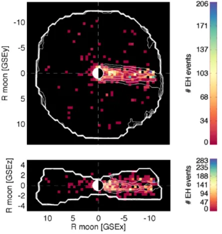
The simulation prediction that kinetic instability in plasma wake behind an unmag-netized object generates electron holes is supported by actual spacecraft data. ARTEMIS mission is a NASA mission of two satellites orbiting the moon. A statistical study of the solitary electrostatic waves encounters by these satellites shows a higher concentration of electron holes in the lunar wake compared to free solar wind. A plot illustration is shown in Figure 1-9. The data show a significantly higher concentration of electron hole events in the lunar plasma wake. The dwell time of satellites is quite uniform around the moon

and the space is uniformly sampled. The results are presented in the Geocentric Elliptic Coordinate system centered around the moon.

Figure 1-9: Event density of electron hole encounters around the moon, colors show the number of events. The contours are iso-density contours for protons showing the shape of lunar wake. Courtesy of David Malaspina.

IV

Other nonlinear solitary wave phenomena in plasma

In this section, we are going to introduce other nonlinear solitary wave phenomena in plasma, with a focus on ion-acoustic solitons. In linear wave theory, the higher order terms in wave amplitude are neglected in linearization. However, when the wave ampli-tude becomes significant, the linear approach breaks down and nonlinear effects must be taken into account. Nonlinearity plays an important role in plasma physics. The BGK mode electron holes we have presented before in this chapter have strong trapped-particle

nonlinearity. Other nonlinearity such as the convective nonlinearity is responsible for the existence of fluid solitons and shock fronts in plasma [59]. Similar nonlinear waves are also actively studied in hydrodynamics for surface water waves [60] and in optics for light pulses traveling in optical fibers [61]. Plasma is inherently a nonlinear medium, which makes the study of nonlinear phenomena in plasma both important and fruitful.

IV.1

Ion-acoustic soliton and the Korteweg-de Vries equation

Ion-acoustic solitons are solitary pulses of ion perturbations traveling at a velocity slightly higher than the cold ion sound speed 𝑐𝑠 = √︀𝑇𝑒/𝑚𝑖. They bear some similarities to

electron holes. As a localized enhancement of ion density, an ion-acoustic soliton carries positive charge and is thus a positive potential pulse. Bipolar electric fields of the same polarity as an electron hole are associated with an ion-acoustic soliton. Its spatial width is also on the order of several Debye lengths. However, it is fundamentally different, because the ion accumulation provides the excess charge in an ion-acoustic soliton and it emerges from fluid equations rather than kinetic ones. To derive the governing equation of an ion-acoustic soliton, we start by assuming that ions are cold (𝑇𝑖 ≪ 𝑇𝑒) and nondrifting relative

to the electrons. Furthermore, electron inertia is neglected (𝑚𝑒 → 0) and electrons are

assumed to be isothermal with an equation of state 𝑃𝑒 = 𝑛𝑒𝑇𝑒. Conservation of electron

momentum under these assumptions gives what is often referred to as the Boltzmann electron approximation for electron density

𝑛𝑒 = 𝑛0exp (𝑒𝜑/𝑇𝑒) , (1.39)

where 𝑛0 is the background electron density. For the ions, we have conservation of density

and momentum equations

𝜕𝑛𝑖 𝜕𝑡 + 𝜕(𝑛𝑖𝑣𝑖) 𝜕𝑥 = 0, (1.40) 𝜕𝑣𝑖 𝜕𝑡 + 𝑣𝑖 𝜕𝑣𝑖 𝜕𝑥 = − 𝑒 𝑚𝑖 𝜕𝜑 𝜕𝑥. (1.41)

To simplify notation, we nondimensionalize the equations with the following normaliza-tion: 𝑛𝑖/𝑛0 = 𝑛, 𝑣𝑖/𝑐𝑠 = 𝑢, 𝑥/𝜆𝐷𝑒 = 𝜂, 𝜔𝑝𝑖𝑡 = 𝜏 , 𝑒𝜑/𝑇𝑒 = Φ. Equations (1.40) (1.41)

together with Poisson’s equation can be written in the dimensionless form 𝜕𝑛 𝜕𝜏 + 𝜕(𝑛𝑢) 𝜕𝜂 = 0, (1.42) 𝜕𝑢 𝜕𝜏 + 𝑢 𝜕𝑢 𝜕𝜂 + 𝜕Φ 𝜕𝜂 = 0, (1.43) 𝜕2_Φ 𝜕2_𝜂 = exp(Φ) − 𝑛. (1.44)

We first look for a solitary stationary solution that travels with a Mach number 𝑀 . A solitary solution implies the vanishing of all perturbations at the boundary, thus we have the boundary conditions: Φ → 0, 𝑢 → 0, 𝑛 → 1 as |𝜂 − 𝑀 𝜏 | → ∞. We integrate Equations (1.42), (1.43) with the boundary conditions and use the calculated density 𝑛 in Equation (1.44). Multiplying Equation (1.44) by Φ′ _{= 𝜕Φ/𝜕𝜂 and integrating with the}

boundary conditions, we have 1

2(Φ

′₎2 _{=[︀exp(Φ) + 𝑀(𝑀}2_{− 2Φ)}1/2_{− (𝑀}2_{+ 1)]︀ . (1.45)}

The right hand side of this equation is minus the Sagdeev potential 𝑉 (Φ) we introduced while constructing an electron hole solution using the differential approach. We look for a solution that travels slightly faster than 𝑐𝑠 with a small amplitude such that Φ ≪ 1

and 𝛿𝑀 = 𝑀 − 1 ≪ 1. Expand Equation (1.45) in Φ and 𝛿𝑀 and integrate it with the solitary boundary conditions; we get

Φ = 3𝛿𝑀 sech2 [︂ (1 2𝛿𝑀 ) 1/2_{(𝜂 − 𝑀 𝜏 )} ]︂ . (1.46)

This is the stationary ion-acoustic soliton solution in small-amplitude limit. It gives the relation between the soliton amplitude and its velocity: 𝑀 = 1+ 𝜓/3. Larger ion-acoustic solitons travel faster. The width of a soliton is of order (𝛿𝑀 )−1/2_{, therefore a faster soliton}

Furthermore, it also gives the scaling of 𝜂 and 𝜏 . We introduce 𝜖 as the scale of 𝛿𝑀 and a new coordinate 𝜉 = 𝜂 − 𝜏 . This is equivalent to changing the reference frame to a moving frame with velocity 𝑐𝑠. The argument in Equation (1.46) can be expressed as

(1/√2)[︀𝛿𝑀1/2_{𝜉 − 𝛿𝑀}3/2_{𝜏]︀. Therefore, the partial derivatives scale like 𝜕/𝜕𝜉 ∼ 𝜖}1/2 _and

𝜕/𝜕𝜏 ∼ 𝜖3/2_{. We can rewrite the equations with the new variables}

𝜕𝑛 𝜕𝜏 + 𝜕(𝑛(𝑢 − 1)) 𝜕𝜉 = 0, (1.47) 𝜕𝑢 𝜕𝜏 + (𝑢 − 1) 𝜕𝑢 𝜕𝜉 + 𝜕Φ 𝜕𝜉 = 0, (1.48) 𝜕2_Φ 𝜕2_𝜉 = exp(Φ) − 𝑛. (1.49)

Now we expand the equations near a stationary solution of small amplitude traveling near 𝑐𝑠. We introduce the following expansions

𝑛 = 1 + 𝜖𝑛(1)_{+ 𝜖}2_𝑛(2)_{+ ... , (1.50)}

Φ = 𝜖Φ(1)_{+ 𝜖}2_Φ(2)_{+ ... , (1.51)}

𝑢 = 𝜖𝑢(1)_{+ 𝜖}2_𝑢(2)_{+ ... . (1.52)}

The lowest order equations with the solitary solution boundary conditions give 𝑛(1) ₌

Φ(1) _{= 𝑢}(1)_{. To next order in 𝜖, the equations can be combined into one nonlinear partial}

differential equation only involving Φ(1)

𝜕Φ(1) 𝜕𝜏 + Φ (1)𝜕Φ(1) 𝜕𝜉 + 1 2 𝜕3_Φ(1) 𝜕𝜉3 = 0. (1.53)

This is the Korteweg-de Vries (KdV) equation, which was first derived by Korteweg and de Vries [62] studying long surface waves in water in a channel of constant depth. It governs a wide range of nonlinear phenomena in physics. The second term Φ(1)_𝜕Φ(1)_/𝜕𝜉

in Equation (1.53) is the nonlinear convective term responsible for wave steepening, the last term 1₂𝜕3_Φ(1)_/𝜕𝜉3 _{is the dispersive term responsible for wave dispersion. A solitary}