Computational learning theory : new models and algorithms

Computational Learning Theory: New Models and

Algorithms

by

Robert Hal Sloan

S.M. EECS, Massachusetts Institute of Technology (1986) B.S. Mathematics, Yale University (1983)

Submitted to the Department- of Electrical Engineering and Computer Science in partial fulfillment of the requirements for the degree of

Doctor of Philosophy at the

MASSACHUSETTS INSTITUTE OF TECHNOLOGY June 1989

@

The author hereby grants to MIT permission to reproduce and to distribute copies of this thesis document in whole or in part.

Signature of Author

Department of Electrical Engineering and Computer Science May 23, 1989 Certified by

Ronald L. Rivest Professor of Computer Science

Thesis Supervisor Accepted by

Arthur C. Smith Chairman, Departmental Committee on Graduate Students

Abstract

In the past several years, there has been a surge of interest in computational learning theory-the formal (as opposed to empirical) study of learning algorithms. One major cause for this interest was the model of probably approximately correct learning, or pac learning, introduced by Valiant in 1984.

This thesis begins by presenting a new learning algorithm for a particular problem within that model: learning submodules of the free Z-module Zk. We prove that this algorithm achieves probable approximate correctness, and indeed, that it is within a log log factor of optimal in a related, but more stringent model of learning, on-line mistake bounded learning.

We then proceed to examine the influence of noisy data on pac learning algorithms in general. Previously it has been shown that it is possible to tolerate large amounts of random classification noise, but only a very small amount of a very malicious sort of noise. We show that similar results can be obtained for models of noise in between the previously studied models: a large amount of malicious classification noise can be tolerated, but only a small amount of random attribute noise.

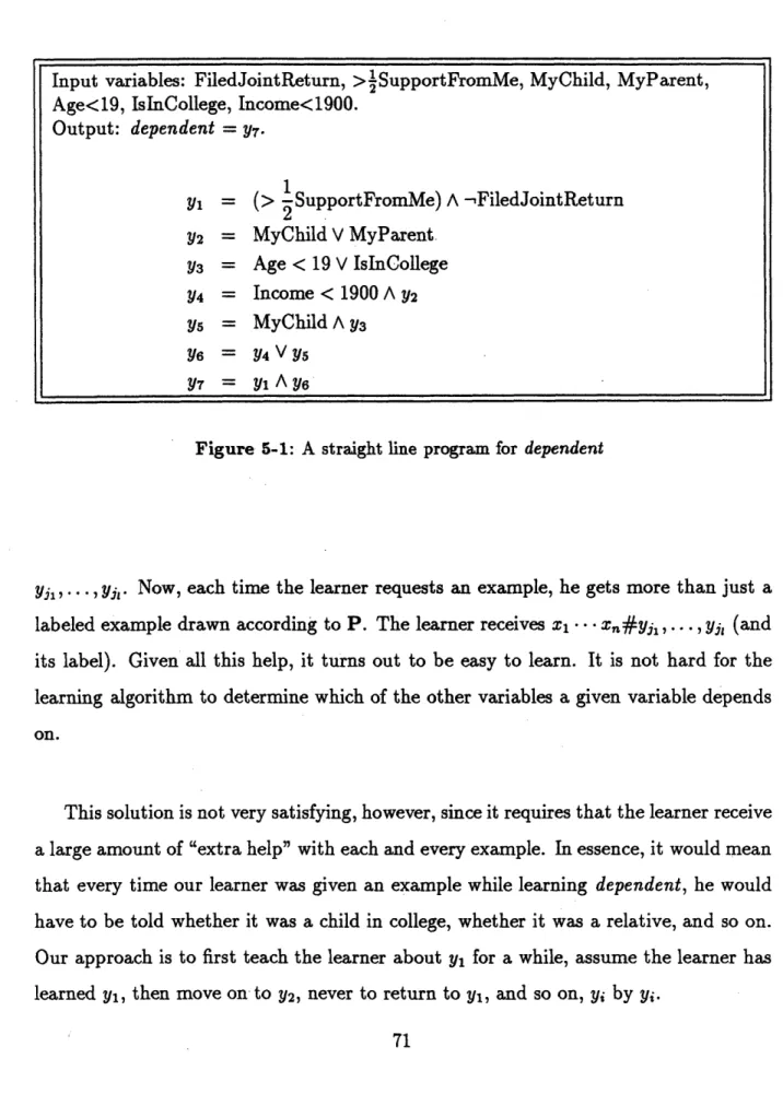
Next, we overcome a major limitation of the pac learning model by introducing a variant model with a more powerful teacher. We show how to learn any concept representable as a boolean function, with the help of a teacher who breaks the concept into subconcepts and teaches one subconcept per lesson. The learner outputs not the unknown boolean circuit, but rather a program which, on a given input, either produces the same answer as the unknown boolean circuit would, or else says "I don't know." Thus, unlike many learning programs, the output of this learning procedure is reliable. Furthermore, with high probability the output program is nearly always useful in that it says "I don't know" on only a small fraction of the domain.

Finally, we look at a new model for an older learning problem, inductive inference. This new model combines certain features of the traditional model of Gold for inductive inference together with the concern of the Valiant model for efficient computation and also with notions of Bayesianism. The result is a model that captures certain qualitative aspects of the classic scientific method.

Keywords: Machine learning, computational learning theory, concept learning, noise, inductive inference, scientific method.

Thesis supervisor: Ronald L. Rivest. Title: Professor of Computer Science.

Acknowledgments

My first and greatest thanks go to my advisor, Ron Rivest. Ron was a pleasure to work with throughout my time at MIT, and much of this thesis was joint work with him. Whenever I was stuck on a problem, Ron had new approaches to suggest. His approach would always be some clever idea that I wished I had thought of; moreover, his clever idea very often solved the problem. In particular, when I was stymied by the problem of learning by subconcepts discussed in Chapter 5, it was Ron who said,

"Well, why not just keep all the possibilities for the right function?"

I was also fortunate to get to work with Manfred Warmuth and David Helmbold. The results of Chapter 3 were joint work with them. I would like to thank the two of them both for their gracious permission to reproduce that work here, and for the fun I had working with them. More generally, I would like to thank both Manfred and David Haussler for inviting me to visit U. C. Santa Cruz in the summer of 1988, where I had many fruitful technical conversations with Manfred and both Davids.

Several people helped me proofread and edit this document. Ron Rivest was ex-tremely helpful in this activity. Additionally, careful proofreading of parts of this thesis by Rob Gross, Maury Neiberg, and Manfred Warmuth resulted in numerous small im-provements in the text.

Finally, I want to acknowledge the funding agencies without whom this sort of research would not occur. I was supported while writing this thesis by an NSF graduate fellowship, and received additional support from NSF grant DCR-8607494, ARO Grant DAAL03-86-K-0171, and the Siemens Corporation.

Contents

1 Introduction 8

1.1 Prologue: An afternoon stroll ... 8

1.2 An introduction to learning theory . ... . 9

1.2.1 W hat is learned ... 10

1.2.2 From what is it learned ... .... 11

1.2.3 What a priori knowledge does the learner have . ... 11

1.2.4 How is what is learned represented . ... 12

1.2.5 By what method is it learned . ... . ... 12

1.2.6 How well is it learned ... 12

1.2.7 How efficiently is it learned . ... .. . 14

1.3 Overview of remaining chapters ... ... 15

2 Pac 2.1 2.2 2.3 2.4 2.5 learning Introduction ... Pac learning ... Discussion of the definition . . . . An example of pac learning ... Some definitions and technical details 2.5.1 Asymptotics ... 17 . . . . 17 . . . . 18 . . . . . 20 . . . . 2 1 . . . . . 22 . . . . 22

2.5.2 Method of sampling . . . . 2.5.3 Samples and consistency . 2.5.4 Variations on pac learning . . . 2.6 Sufficient conditions for pac learnability 2.6.1 Occam algorithms . . . . 2.6.2 VC dimension . . . . 3 A learning algorithm for submodules

3.1 Introduction . .. .... 3.2 Mistake bounded learning 3.3 Learning submodules . . . 3.3.1 The algorithm SM 3.3.2 Running time . . . 3.3.3 Mistake bound . . 3.3.4 Special case: k = 1 3.3.5 Generalizations . . 3.4 Applications of modules . 3.4.1 Abelian groups .

3.4.2 Some commutative languages 4 Learning from noisy data

4.1 Introduction ... 4.2 Notation ... 4.3 Main results...

4.3.1 Attribute noise . . . . 4.3.2 Misclassification noise . . . . . 5 Learning concepts reliably and usefully

5 32 32 53 53 54 57 57 60 .

5.1 Introduction 5.1.1 5.1.2 Hierarchical lea A new variatio: arning . . . . n on the Valiant model .

. . . . . . . . . . . . . .

5.2 How to learn: sketch 5.2.1 Notation ...

5.2.2 An easy but trivial way to learn . . . 5.2.3 High level view of our solution . . . . 5.3 Detailed specification of our learning protocol

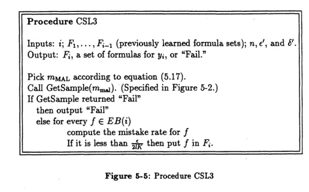
5.3.1 Learning y. . . . . 5.3.2 Learning the target concept . . . . . 5.3.3 Removing the circuit size as an input 5.4 N oise . . . .

5.4.1 Classification noise . . . . 5.4.2 Malicious noise . . . . 5.5 Summary and conclusions . . . . 6 A different model of learning

6.1 Introduction ...

6.2 Subjective probabilities .. . . . . 6.3 The M odel ...

6.3.1 Basic Notation and Assumptions ... 6.3.2 The Scientist Makes Progress .. . . . . . 6.3.3 How Long Will Science Take? . .. . . . . 6.3.4 How the Scientist Updates His Knowledge 6.3.5 An Example .. . . . . 6.4' Our Inference Procedures .. . . . . 6.4.1 General Assumptions .. . . . . 6 91 91 93 94 94 94 95 96 97 98 99 . . .

6.4.2 Optimization Criteria... 99

6.4.3 Menus of Options ... ... .. 100

6.5 Inference procedure 1: Maximizing the weight of refuted theories .... 101

6.5.1 A Simple Menu of Options ... ... 101

6.5.2 An Expanded Menu of Options . ... 102

6.5.3 Behavior of this Inference Procedure . ... . 104

6.6 Inference procedure 2: A minimum entropy approach . ... 106

6.6.1 Behavior of this Inference Procedure . ... . 107

6.7 Inference procedure 3: Making the best theory good ... .. 109

6.7.1 Behavior of this Inference Procedure ... . 110

6.8 An optimality result ... 112

6.8.1 The optimal refutation rate . ... . 112

6.8.2 How our procedures compare to the optimum . ... 113

6.9 Conclusions for Chapter 6 ... ... 114

Chapter 1

Introduction

Learning is not attained by chance, it must be sought for with ardor and attended to with diligence.

-ABIGAIL ADAMS, Letter to John Quincy Adams

1.1

Prologue: An afternoon stroll

It is a bright, sunny afternoon. I take my robot out for a walk with me. We stop and sit down on a bench in a busy part of town. For every person who walks by us I say to my robot either, "That's a male," or "That's not a male," as the case may be. We stay quite some time, and eventually go home.

The following afternoon the weather is the same, and we go back to the same bench. This time, for every person who walks by, my robot says to me either "That's a male," or "That's not a male." My robot is correct ninety-six percent of the time.

It seems fair to say that my robot has learned the concept male, or at least a close approximation of that concept. One of the main subjects of this thesis will be what algorithms a robot might use to accomplish such learning.

1.2

An introduction to learning theory

Formally, the subject of this thesis is computational learning theory. For our pur-poses, learning means induction. The task of a learner is to sample some portion of the world, or whatever more limited domain may be under consideration, and come to some conclusion about the nature of the entire domain. What distinguishes compu-tational learning theory is that one of the efficiency issues that we care about is how much computation time the learner uses. Our goal is twofold: we want to specify in-teresting formal models of the problem of learning, and we want to present algorithms for achieving learning within these models.

All of the problems we study in this thesis can be fit into the following broad pattern. There is some universe of objects that is under consideration. We call this set the instance space or the domain. The domain might be the set of points in the real plane, bit vectors, the set of all the fish in the Boston Aquarium, or the set of all human beings on earth. The elements of the domain are called instances. These instances are split into two categories: positive instances and negative instances. The set of positive instances is called the target concept. Our learner receives as input a sample of instances with labels that tell whether they are positive instances or negative instances. We call such labeled instances examples. The goal of the learner is to to find some rule which distinguishes positive instances from negative instances.

For instance, in the example given above in the Prologue, the domain is the set of all people, and the positive instances are male people. In that case I did not demand that the learner come up with a completely accurate rule for classifying people; I was happy with a good approximation.

There are several issues we must consider before we have posed a well specified learning problem. In particular, Rivest [46] suggests that (at least) the following seven questions must be answered in order to specify a learning problem.

1. What is being learned?

2. From what is it learned?

3. What a priori knowledge does the learner begin with?

4. How is what is learned represented?

5. By what method is it learned?

6. How well is it learned?

7. How efficiently is it learned?

We now briefly examine each of these questions in turn.

1.2.1

What is learned

There are many different domains one may study learning for. One might be interested in learning about people or maps or nuclear particles. This thesis is a theoretical work, and we examine exclusively abstract mathematical domains such as bit vectors, Euclidean n-space, and k-tuples of integers. We study these domains both because they are interesting in their own right, and in the belief that they are rich enough to form good mathematical models of real world problems.

For instance, the robot discussed in the Prologue presumably would represent people as a feature vector which includes (at least) real, integer, and boolean valued compo-nents. The problem of choosing a good representation is both fascinating and difficult-indeed, it is one of the central problems of Artificial Intelligence-but it falls outside the scope of this thesis.

1.2.2

From what is it learned

The data our learner gets consists of labeled instances. As noted above, these instances come from various abstract mathematical domains. We generally ignore the details of how these instances are represented, and just assume some reasonable fixed encoding scheme.

We are, however, very concerned with the issue of how training examples are chosen from the domain. If the examples are chosen to be extremely helpful, then philosophi-cally one might object that what is going on is programming rather than learning. A more practical objection is that we now have the problem of finding a teacher capable of picking out such extremely helpful examples. On the other hand, if the examples are not somewhat representative of the whole domain, then the learning task may be infeasible.

Another issue that sometimes arises is whether the learner is given both positive and negative training examples or only positive examples. Which is more natural depends on the domain. In the case of learning to distinguish male people, both positive and negative training instances would presumably be available. On the other hand, in the case of learning to distinguish well formed English sentences from nonsense sounds, only positive instances might be available.

We are also interested in what happens when there is some noise in the training data. For obvious reasons we prefer learning algorithms that are robust against some amount of noise.

1.2.3

What a priori knowledge does the learner have

Our learner does not necessarily begin its' work in a state of total ignorance. For instance, we often help the learner by telling it ahead of time that the target concept

comes from some particular class of concepts. (More formally, we design learning algorithms that are only guaranteed to work on the assumption that the target concept comes from some particular class.) Some limiting of the class of possible concepts is clearly necessary. If any subset of the instance space could be the target concept, and if all such subsets were equally likely, then the learner would have no basis whatsoever for performing its induction.

Another sort of initial knowledge a learner may have consists of a priori probabilities of the truth of various propositions such as "Concept c is the target concept."

1.2.4

How is what is learned represented

In some cases we are happy if the learner outputs any representation of the target concept. Sometimes, however, we further complicate the learner's task by requiring that its output be in some particular form. In particular, when it is known a priori that the target concept is representable in some special form (for instance, a boolean formula in 3DNF), we may require that the learner's output also be in that form.

1.2.5

By what method is it learned

The answers to the previous questions determine a learning problem. Our goal is then to find a solution to that problem: an algorithm that learns according to the definition of learning given by our answers to the previous questions.

The goal of computational learning theory in general, and this thesis in particular, is to pose interesting learning problems, and to find algorithms that solve those problems.

1.2.6

How well is it learned

A learning algorithm is a proposed solution to a problem in learning. Having proposed a solution, one must next ask how good that solution is.

Two very different notions of learning well have been studied. In one, generally called inductive inference, the learner is given a presentation of examples one at a time indefinitely, and its goal is to converge in the limit to the correct rule for classifying instances. Inductive inference was first studied by Gold [14], and it has received con-siderable attention since then. For the most part we are not concerned with inductive inference in this thesis (although it was one of the inspirations for the model we study in Chapter 6). For interested readers, [6] is an excellent survey article; an excellent introductory book on the subject is [39].

In this thesis, we are instead concerned with what is generally known as learning concepts from examples or simply learning from examples. The learner receives only some limited number of examples, and after that is supposed to output some represen-tation of a rule for distinguishing positive instances from negative instances. Intuitively, the idea is that the presentation of the labeled instances constitutes the training of the learner, and that after training the learner should be able to classify previously unseen instances for itself.

In the context of learning from examples, we normally call the rule for distinguishing positive from negative instances a concept. As mentioned above, the true rule is called the target concept. To decide whether the learner has learned well, we may ask simply whether the learner has produced as output some representation of the target concept. Learning, however, is a difficult task, and unless the task is highly constrained, always finding exactly the target concept concept may be difficult or even impossible. (Re-member that the whole point of learning from examples is to avoid showing the learner all possible instances in the training phase.) Thus we often settle for the learner out-putting a concept that is "close to" the target concept, or even "probably" close to the target concept. Of course, "close to" and "probably" must be precisely defined in any particular formal model of concept learning.

measure whether those criteria have been met. One obvious approach is to imple-ment any proposed learning algorithm and then run it on test data. Much artificial intelligence research on machine learning follows that empirical approach.

This thesis, however, contains no empirical results at all. Instead, we give formal

proofs that our algorithms meet various criteria for learning well. The emphasis on

proving the goodness of algorithms is, in fact, one key property that distinguishes computational learning theory from other machine learning research.

1.2.7

How efficiently is it learned

In addition to requiring the learner to learn well, we also require the learner to learn efficiently. There are three sorts of resources the learner consumes:

1. Computation time.

2. Memory.

3. Labeled instances.

We require that our learner be restricted to efficient computation. At the present time, "efficient computation" is generally understood to mean whatever can be com-puted in probabilistic polynomial time (technically BPP). That is the restriction we impose on all learning algorithms studied in this thesis. Of course, in order to re-strict our learner to probabilistic polynomial time computations, we have to answer the question, "Polynomial in what?"

For the most part, we are content simply with finding algorithms that meet the broad BPP definition of efficient, and ignore the question of the particular asymptotic running times of our algorithms, though we occasionally discuss running times. Notice that this approach is may be unrealistic if one's goal is to actually build real-time robots.

Similarly, we generally ignore the memory usage of our algorithms. The running time of an algorithm places a crude bound on its memory usage, and we settle for that. In addition to the usual resources of time and space, learning algorithms also con-sume labeled instances. The number of instances concon-sumed forms an obvious lower bound on the running time of an algorithm, so we restrict all our algorithms to a polynomial number of instances.

In the other direction, we study how many examples must be present to solve certain learning problems. Just as the problem of sorting has an Q (n log n) lower bound on its time complexity-independent of how much memory a sorting algorithm has available-certain learning problems have various lower bounds on their sample complexity independent of how much time or memory they have available. Intuitively a particular sample complexity for a learning problem means that at least that much data are required for a statistically adequate sample.

1.3

Overview of remaining chapters

In the next chapter we formally specify a particular model of concept learning, Valiant's pac learning model [52]. That model addresses many of the concerns discussed in this introductory chapter.

In Chapter 3 we exhibit a learning algorithm for learning a certain class of concepts within the pac learning model. The instance space is Zk, or more generally, any Eu-clidean domain, and the concepts of interest are any submodule. We give a detailed analysis of the performance of the algorithm, and the lower bounds for the problem it solves, and examine several applications of the algorithm. We show that this algo-rithm is optimal within the pac learning model, and near optimal in a related but more stringent learning model called on-line learning.

model was published, several authors have considered the effects of noisy data within that model [51, 5, 25, 31]. Those papers all assumed one of two particular types of noise that might corrupt the data: one very malicious, and one very benign. Not surprisingly, it was shown that the maximum tolerable amount of noise is much greater for the benign model than for the malicious model. In chapter 4, we consider where the dividing line between these models falls. In particular, we study two new models of noise, both "in between" the models previously studied.

One limitation of the pac learning model is that certain learning problems are computationally intractable in that model. In Chapter 5, we specify a learning model with a more helpful teacher than the one allowed in pac learning. With the aid of this teacher, we be able to learn any reasonable concept class, and also achieve a stronger sort of learning than pac learning.

Finally, in Chapter 6, we look at an altogether different type of learning. In that chapter we introduce a new model of learning that combines certain aspects of learning from examples and inductive inference. The result is something that crudely models the scientific method.

Chapter 2

Pac learning

2.1

Introduction

In this chapter we formally define one particularly important model of learning, "prob-ably approximately correct learning," or pac learning for short [52]. All of the results in this thesis except for those in Chapter 6 are in either the pac learning model or some variation thereof. We briefly discuss the intuition behind the pac model, and then give an example of an algorithm for a particular learning problem within this model, learning monomials.

Next we discuss a number of technical issues of pac learning. These issues are important in Chapter 4 where we discuss the effect of noisy data on pac learning algorithms, and in Chapter 5 where we discuss a variation on the pac learning model.

We conclude by discussing sufficient conditions for pac learning, including the im-portant combinatorial parameter known as the Vapnik-Chervonenkis dimension [55). An understanding of that parameter is necessary for some of the results in Chapter 3. With the exception of Theorem 2.2, which is original, the material in this chapter is all a review of the computational learning theory literature.

2.2

Pac learning

In an influential 1984 article [52], Valiant introduced the pac learning model. In short, an algorithm pac learns from examples if it can, in a feasible amount of time, find (with high probability), a rule that is highly accurate. Now we must define what we mean by such terms as "find a rule," "with high probability," and "highly accurate."

Fix an instance space X. Formally a concept c for instance space X is some subset of X. If instance x E X is contained in concept c, then we say that x is a positive instance of c; otherwise we say that x is a negative instance of concept c. (We are slightly sloppy throughout and refer to concepts interchangeably both as subsets of the instance space and as {0, 1}-valued functions defined on the instance space.)

The length of concept c, denoted Icd, is the number of bits it takes to write down c in some agreed-upon encoding scheme. For example, if our instance space is {0, 1}", pos-sible representations for concepts include truth tables, boolean formulas, and boolean circuits. (Haussler [20] gives a good discussion of issues concerning choice of represen-tation of concepts.) The length of an instance is defined similarly.

Let C be a set of concepts or concept class over X. Formally, C C 2x . _{If X is} the inhabitants of the U. S., concepts would include both the rather simple concept males, and the doubtless more complicated concept, people whose marginal federal income tax rate is thirty-three percent. An example of a concept class would be TAX BRACKETS which would include the concepts people paying no income tax and people whose marginal tax rate is thirty-three percent.

We call the concept c E C that our algorithm is trying to learn the target concept. The target concept may be any concept whatsoever in the concept class. We think of it as being arbitrarily chosen by some outside teacher or supervisor.

We assume that our learning algorithm has available to it a black box called EX-AMPLES, and that each call to the black box returns a labeled example, (x, s), where

x E X is an instance, and s is either "+" or "-" according to whether x is a positive or negative instance of the target concept c. Furthermore, the EXAMPLES box generates the instances x according to some fixed probability distribution P on X. We make no assumptions whatsoever about the nature of P, and our learner is not told what P is. First we define formally what it means for a concept to be an accurate approximation of target concept c, and then we define pac learning itself.

DEFINITION. Fix an instance space X and a probability distribution P on X. We say that concept cl is an e-approximation of concept co if and only if

S

DEFINITION. Let C be a class of concepts on domain X. Algorithm A probably approximately correctly learns (pac learns) C if and only if for every c E C, for every probability distribution on X, for every positive e and 6, algorithm A, given only e, S and access to EXAMPLES(c), meets the following two criteria.

Learning criterion Algorithm A outputs some representation of a concept c' such that

Pr [c' is an e-approximation of c] > 1 - 6 (2.2) where the probability is taken over the output of EXAMPLES and any coin tosses A may make.

Efficiency criterion The running time of A is bounded by some polyno-mial function of 1/e, 1/6, the length of an instance, and the length of the target concept.

We say that a concept class C is pac learnable if there exists some algorithm that pac learns C.

We note here for later use the following weaker definition.

DEFINITION. Statistical pac learning or s-pac learning is defined the same as pac learning except that the efficiency criterion is that the sample complexity rather than the running time must be bounded by by some polynomial function of 1/e, 1/6, the length of an instance, and the length of the target concept.

2.3

Discussion of the definition

Intuitively, we are saying that the learner is supposed to do the following: 1. Ask nature for a random set of examples of the target concept. 2. Run in polynomial time.

3. Output some concept that with high probability agrees with the target concept on most of the instances.

We think of Nature as providing examples to the learner according to the (unknown) probability with which the examples occur in Nature. Though the learner does not know this probability distribution, he does know that the concept he outputs needs to closely approximate the target concept only for this probability distribution.

Intuitively, there may be some extremely bizarre but low probability examples that occur in Nature, and it would be unreasonable to demand that the learner's output con-cept classify them correctly. Hence we require only approximate correctness. Moreover, since the examples the learner receives from Nature are drawn stochastically, there is some small but nonzero chance that those examples will be wildly unrepresentative. Therefore we cannot require the learner to always output an approximately correct concept; we only require that the learner do so with high probability.

The notion of s-pac learning was studied in the statistical pattern recognition liter-ature before the notion of pac learning was introduced in 1984. The difference between

the two is that s-pac learning requires us to be efficient in our consumption of examples but not in our computation time. Notice that any algorithm that pac learns must s-pac learn since the sample complexity of an algorithm is a lower bound on its running time. Thus the strongest infeasibility results we can obtain are showing the infeasibility of s-pac learning. In general it is often easier to prove theorems about s-pac learning than about pac learning.

The excellent survey article of Kearns et al. gives a more lengthy discussion of the entire pac learning model, and also provides an overview of recent results obtained using this model [26]. Blumer et al. and Valiant both contain additional material on the motivation for the pac learning model [9, 52].

2.4

An example of pac learning

We now exhibit an algorithm that pac learns monomials [52]. The instance space is {0, 1}" for some positive n. The concept class is the set of all boolean expressions in n variables that can be represented as monomials (simple conjunctions of literals).

The algorithm A for pac learning is as follows: A first makes one call to EXAMPLES, and figures out what n is. (Alternatively, n may be an additional input to A.) A then initializes its hypothesis to be the conjunction of all 2n literals, x1 1 - z,,. A then

makes m more calls to EXAMPLES, where 1

m = - (n In 3 + In(.1/)).

For each positive instance, (instance, +), algorithm A crosses off zx from its hypothesis if xi is 1 in instance, and crosses off ti if xi is 0 in instance. Algorithm A simply ignores negative instances. The output of A is the monomial consisting of whatever literals have not been crossed off after the m instances are seen. (If all of the m instances are negative, then A's hypothesis is xz1E ... 2,i, which is always false.)

The running time of of A is clearly polynomial in 1/, 1/6, and n, and the length of an instance is n, so A meets the efficiency criterion for pac learning. It follows easily from the results of Blumer et al. [11] that A meets the learning criterion for pac learning. The value of m is not the best possible, but it makes the proof especially simple.

2.5

Some definitions and technical details

2.5.1

Asymptotics

Throughout, we strive to find computationally efficient learning algorithms. We there-fore need to discuss the asymptotic difficulty of our problems. Otherwise, all problems can be solved in "constant" time.

For instance, the concept class COly• of all subsets of {0, 1}n accepted by some polynomial-size circuit is not pac learnable if any one-way function exists (Valiant [52] using cryptographic tools of Goldreich, Goldwasser, and Micali [15]). Nevertheless, if we simply fix n, in spite of that result, it would be possible to pac learn the class

CP°ly. The running time of the algorithm to do so would be a particular polynomial function of 1/f and 1/6. That polynomial would, however, contain some multiple of the "constant" 2" as one of its coefficients.

Thus instead of examining algorithms for one fixed learning problem, we always examine algorithms for an infinite sequence of learning problems. There are two differ-ent ways we can construct this sequence: by allowing instance length to grow and by allowing concept length to grow.

In the first approach we must parameterize the instance space. Thus our instance space X = Ulo X,. We assume that there is some polynomial 1 such that all instances in X, have length between n and l(n). We also assume that any one concept c in

our concept class C is completely contained in X, for some n. We define C,,• to be {c E Clc C X, and Icd < s}, and C, = U,C,,,. Various classes of boolean functions are often studied in this way. Another example of a concept class that can be studied this way is the class of half-spaces of R". We note for future reference that we consider such

a concept class to be finite if ICnI is finite for every n.

The other way to make our learning problems asymptotic is to take a fixed instance space, but to allow concepts to grow arbitrarily complex. For instance, we could fix the instance space to be the real plane, and let C be the set of all convex polygons. We could then make C, the set of convex n-gons, or alternatively, the set of convex polygons with at most n edges.

2.5.2

Method of sampling

Notice that our definition of pac learning did not require that the learning algorithm make all its calls to EXAMPLES at once. Indeed, the pac learning algorithm we gave for learning monomials first makes one call to determine the length of instances, and then makes m further calls, where m is dependent on what that first call to EXAMPLES returned.

Early work in pac learning generally required that a learning algorithm make a fixed number of calls to EXAMPLES dependent only on the size of instances, e, and 6. We refer to that model of learning as static sampling pac learning. Note that in the static model, the size of an instance is normally an additional input parameter. Linial, Mansour, and Rivest [33] discuss the ramifications of allowing arbitrary calls to EXAMPLES instead of requiring static sampling.

2.5.3

Samples and consistency

For a fixed target concept ct, we call a set of instances each labeled positive or negative a sample (of ct). Whenever there is an underlying probability distribution on the instance space, a sample is assumed to be randomly drawn according to that probability distribution. The size of a sample is the number of instances it contains. Notice that in the usual case where the sample is obtained stochastically, the number of distinct instances in the sample may be less than the size of the sample.

We say that a concept c is consistent with a given sample if c contains all the positive instances in a sample and none of the negative instances. The consistency problem for a concept class is to find a consistent concept for a given sample of some concept in the class.

2.5.4

Variations on pac learning

The pac learning model itself can be altered in many ways. For instance, instead of having a single probability distribution on the whole instance space and a single box EXAMPLES, there can be two separate probability distributions, one each for positive examples and negative examples, and two boxes, EXAMPLES' and EXAMPLES-, each giving only one kind of instance. In this case, the learning algorithm is allowed to make calls to either box, and its hypothesis is required to come within e on both positive and negative examples. This model is called the two-button model; the model we discussed first is called the one-button model.

There are in fact numerous different minor variations on pac learnability. Haussler et al. compare many of these variations, and show them to be substantially equivalent.

2.6

Sufficient conditions for pac learnability

Let us briefly examine when a concept is pac learnable. A starting place place is the case when the concept class has very small cardinality. In the extreme, consider the case where the concept class contains only two concepts, cl and c2.

In general, we are concerned only with situations where it is computationally effi-cient to determine whether any particular instance is contained in a given concept. Let us assume that is the case for cl and c2. Now all we need to do is draw a sufficiently

large sample from EXAMPLES, and select whichever concept is consistent with the sample, or, if both concepts are consistent, choose either one arbitrarily.

We can extend this line of reasoning to considerably larger (finite) concept classes. Our treatment follows Blumer et al. [11]. Consider an algorithm that draws a sample of size m(CI , _{, 8), and then outputs any concept c E C that is consistent with the}

sample. Ignoring for a moment the issue of computation time, what is a lower bound on the function m that insures that the learning algorithm meets the s-pac learning condition?

DEFINITION. Fix a target concept and a probability distribution on the instance space. We say that a concept is e-good if it is an f-approximation of the target concept, and f-bad if it is not.

We want to guarantee that the probability that the algorithm returns an f-bad con-cept is at most 6. The probability that a particular E-bad concon-cept would be consistent with m randomly drawn examples is bounded above by

(1 - E).. (2.3)

A crude upper bound on the probability that any e-bad concept is consistent with m randomly drawn examples is

Hence we want to choose m large enough to insure that

ICl (1 -~) m _{< 6. (2.5)}

Taking logs of both sides, and solving for m yields 1

m (>

ln(ICi)

We can write a simpler inequality that implies inequality (2.6) by noticing that by Taylor's Theorem

(

In

>

Hence a sufficient condition is

m > (In(C) + In

.

(2.7)

We say that m is an upper bound on the sample complexity of the concept class C. More generally we say that an arbitrary concept class V has sample complexity at most m if there is a learning algorithm with sample complexity m that s-pac learns E.

Let us assume that we have an instance space, such as {0, 1}", where all instances have length n, and the length of every concept in our concept class C is bounded by some polynomial function of n. As long as ICl = O (2P()), for some polynomial p, then C has polynomial sample complexity. If C has polynomial sample complexity, and if the problem of finding a concept from C consistent with a given sample can be solved in polynomial time, then C is pac learnable. We call any pac learning algorithm that draws a sample of size m(e, 6, ICI) for some function m, and then returns an arbitrary c E C that is consistent with the sample a static consistent learning algorithm.

There are at most 3' different monomials on n boolean variables, so the concept class of monomials has polynomial sample complexity. The algorithm for learning monomials given above in Section 2.4 is a static consistent algorithm. It draws a sample of a size that meets the bound of inequality (2.7), and in polynomial time finds a monomial consistent with that sample.

On the other hand, the class of all boolean functions on n variables has size 22', so we can not hope to find a static consistent algorithm for it of this sort.

2.6.1

Occam algorithms

A static consistent algorithm draws a sample, and outputs some hypothesis consistent with that sample. There is a more general class of algorithms with that behavior which achieve pac learning, the Occam algorithms [11].

DEFINITION. An Occam algorithm for C with constant parameters c > 1 and 0 < a < 1 is an algorithm that:

1. produces a concept (not necessarily from C) of length at most ncrm when given a labeled sample of length m of any target concept in C of length at most n, and 2. runs in time polynomial in the length of the concept.

The importance of Occam algorithms is shown in the following theorem of [11]: Theorem 2.1 (BEHW) Any Occam algorithm for C pac learns C.

Notice that static consistent algorithms are the special case of Occam algorithms with a = 0.

Observe that an Occam algorithm A must be a data compression algorithm. If we get a sample of labeled instances we can compress it by storing just the instances and the concept output by the Occam algorithm. To decompress we use the concept to recover the original labels.

In particular, the definition of Occam algorithm implies that there is a constant 0 < p < 1 such that for every n, for all sufficiently large m, on input a sample of length m of a concept of length at most n algorithm A must output a consistent concept of length at most m . We know that the length of A's output can be at most nCme for

1--a n"

some a < 1. Now for any fixed n, for sufficiently large m, m - > nc. Thus setting

S= (1 + a)/2 suffices.

In general there is a strong connection between the ability to compress and the ability to learn. Indeed, the ability to compress the sample somewhat is a necessary condition for at least static sampling pac learning.

Theorem 2.2 Let C = U==LC,. be a concept class where C, is defined on {0,1}". If C is statically pac learnable, then there must be an algorithm A such that for every sufficiently large n, there exists a constant e > 0 such that for sufficiently large m, given a sample of length m of any concept c E C,, algorithm A with probability at least

1- 1nl-w(1_{)* returns some representation of a hypothesis of length at most (1- 6)m that}

is consistent with the sample.

Proof We employ cryptographic tools from Yao's theory of "computational informa-tion theory" [57] to show that if such an algorithm does not exist, then we cannot hope to pac learn (or even weakly approximate) C.

For each n, let the probability distribution P on {0, 1}' be the uniform distribution, and fix some concept c, E C,. For n > 1, let Sn+1 be a device that stochastically generates a string consisting of an instance x chosen randomly from {0, 1}" followed by cn(x). Let X1 be an arbitrary stochastic source of strings of length 1. Then S =

SI, S2,... forms a uniform source ensemble. That is to say, each S, is a stochastic *Recall that f(n) = w(g(n)) if and only if g(n) = o(n). In particular, f(n) = In- _{'W(1) if and only}

if f(n) vanishes faster than the reciprocal of any polynomial in n, or, formally, if for every positive c,

source of strings of length n. (For the precise definition see either Yao [57] or a text on information theory.)

Let the true random number ensemble (on alphabet {0, 1}) be the source ensemble R = R1, R2,... where RP assigns probability 2-" to strings of length n and probability

0 to all other strings.

Claim: If S is polynomial indistinguishable from R, then concept class C is not statically pac learnable.

We show the contrapositive of this claim. Assume that we have an algorithm SPL that statically pac learns C. Then we can use algorithm SPL as a subroutine in an algorithm to distinguish S from R. Let s(n, E, 6) be the number of instances from EXAMPLES that SPL requires.

The distinguishing algorithm will work to distinguish samples of S, from samples of RJ as long as the sample length is at least 1 + s(n - 1, 1, -). The behavior of the distinguishing algorithm is as follows: We feed all the labeled examples in the sample except the last one to SPL, to obtain an output concept &. The distinguishing algorithm outputs 1 if the classification of the last instance in the sample.according to C matches its true classification, and 0 otherwise. If the sample came from S,, _{then the output of} the distinguishing algorithm must be 1 with probability at least (1 - !)(1 - 14) = 9 On the other hand, if the the sample came from the true random number ensemble, then the output of the distinguishing algorithm is 1 with probability exactly .

Hence it must be that S _{is polynomial distinguishable from the true random number}

ensemble. Yao [57] shows that this implies that it must be possible to communicate a sufficiently long sample from Sn from one polynomial time computing agent to another using polynomially fewer bits than are in the sample with overwhelming probability. (The probability is taken over the output of the source and over any coins the two communicating parties may toss.) In particular, for sufficiently large m, it must be possible with probability at least 1 - Inj-_w(1_{), to communicate a sample of of length}

m (containing mn bits) in at most m(n - 1/nk) _{bits for some positive integer k. Now}

of the mn bits, m(n - 1) bits come from drawing randomly from {0, ₁}n-1, and so cannot be compressed at all. That means that it must be possible to write down some representation of the m label bits in at most

[m(n -

/nk)

-

m(n - 1) = m(l -

lnk)

bits. Putting e = 1/nk yields the desired result. O

2.6.2

VC dimension

Previously we have examined sufficient conditions for pac learnability. In this section we examine a combinatorial parameter that provides a necessary and sufficient con-dition for static sampling pac learnability, the Vapnik-Chervonenkis dimension [55], hereinafter VC dimension or VCdim. Since it is a combinatorial parameter of set sys-tems, we define it in terms of sets, though of course the sets we are interested are concepts.

DEFINITION. Fix a domain X, and let C C 2x.A set S C X is shattered (by C) if for each subset S' C S, there is a set c E C which contains all of S', but none of the points in S - S'.

Remark: The term shatter is now well established. However, as Pollard points out [43], the right picture to keep in mind is not really S being broken into lot of tiny pieces by C. Rather, one should imagine a diligent C picking out all the different subsets of S. DEFINITION. The VC dimension of C C 2x is the cardinality of the largest set of-points from X shattered by C.

Examples: The class of all rectangular regions in the plane has VC dimension 4. The class of all spheres in R" has dimension n + 1. For any finite concept class C, we

have VCdim(C) <

log(ICl).t

The VC dimension was first studied in connection with statistical pattern recogni-tion. Pollard and Vapnik have both written good books discussing it from that point of view [43, 54]. The first source that I am aware of to point out that it has some connection to efficient concept learning is Pearl [40].

The key fact about the VC dimension for our purposes is that a concept class has polynomial sample complexity if and only if it has finite VC dimension. In particular, if the VC dimension of concept class C is d, then Blumer et al. [10] showed that the sample complexity of C is bounded by

sample complexity < max

(

log

(),

j log

(-)).

(2.8)

Notice that since finite VC dimension is a necessary and sufficient condition for polynomial sample complexity assuming the static sampling model, finite VC dimension is a necessary condition for static sampling pac learnability. It is not, however, a sufficient condition. We must also be able to find a concept consistent with any sample in probabilistic polynomial time. For some concept classes, such as monomials, we know how to do this. However, for many interesting concept classes the problem of finding a concept consistent with a sample is NP-complete.

Chapter 3

A learning algorithm for

submodules

3.1

Introduction

In this chapter we present an algorithm for learning the concept class Ck of all subsets of

Zk closed under addition and multiplication by integers. In algebraic terms Ck consists of all submodules of the free Z-module of rank k. Using other terminology, Ck is the set of all integer lattices contained in R k.

We give a learning algorithm that has performance within a log log factor of optimal in the on-line mistake bound model of learning, which we describe below. That learning model is "more strict" than the pac learning model: any learning algorithm with good performance in the mistake bound model can be used as a subroutine to construct a pac learning algorithm, but not all pac learning algorithms have good mistake bounds. In particular, we prove an absolute mistake bound for the algorithm we present of k log n, where n is an upper bound on the absolute value of any component of any example seen, and prove that no learning algorithm can have a mistake bound of less

than (1 - e) _loglognklog, for any e

>

The algorithm we present has a certain high level similarity to the so-called L3 algorithm for lattice basis reduction [32]. In both cases a tentative basis for the lattice is maintained at all times, and certain algebraic transformations are made to the basis. However, the similarity is only superficial, because the L3 algorithm in fact is solving a very different problem. The goal there is to find an new basis for the same lattice containing one vector of small Euclidean norm. In the learning problem, our goal is to converge towards a basis for the lattice of all positive instances, and every time we update our basis, the lattice generated by the it will strictly increase.

In addition to the algorithm, we also present several applications. For instance, an interesting subclass of the above class Ck is the class Ck' of zero-reversible commutative regular languages over alphabets of size k. (A sufficient but not necessary condition for a commutative regular language to be zero-reversible if for it to have an accepting DFA in which the only final state equals the start state.) Recently it has been shown by Pitt and Warmuth that for any fixed polynomial

Q,

3.2

Mistake bounded learning

There are many ways we can evaluate how well a learning algorithm has learned. We list below four possible criteria, in what intuitively appears to be the order of increasing

strictness.

1. Pac learnability-the learning algorithm must with high probability produce a hypothesis of small error [52].

2. The probability of making a mistake on predicting the label of the last instance

[22].

3. The expected total number of mistakes for on-line prediction of the labels of the first t instances [22].

4. The worst case total number of mistakes for on-line prediction of the labels of any (possibly infinite) sequence of instances [34].

In fact, Haussler et al. [21] have shown that the first two criteria are substantially equivalent. In this chapter we present an algorithm that learns well with respect to the fourth, ,strictest, criteria. It follows that this algorithm can be easily converted to a pac learning algorithm.

We follow Littlestone [34] in defining mistake based performance criteria for learning algorithms. In particular, for learning algorithm A and target concept c define MA(c) to be the maximum number of mistakes algorithm A makes for any possible sequence of instances. For any non-empty concept class C, define MA(C) = maxEc MA(c). Any bound on MA(C) is called a mistake bound for algorithm A applied to class C. The optimal mistake bound for concept class C, opt(C), is the minimum over all learning algorithms A of MA(C).

3.3

Learning submodules

We now present algorithm SM for the on-line learning of the concept class Ck of submodules of the free Z-module Zk. The main data structure this algorithm uses is a

k by k upper triangular matrix M which is initially all 0, and gradually has nonzero rows added to it as we see positive examples. At any point the algorithm's current hypothesis is the row span of M. Algorithm SM makes a mistake only when it gets a new positive example x is not in the span of M. When this happens, M must be updated to a matrix whose span also includes x. Sometimes we can accomplish this by simply adding x as a new row; more often we have to perform an operation similar to Gaussian elimination.

We begin by giving a precise description of algorithm SM in section 3.3.1, and then move on to analyze its mistake rate and give several applications. Note that the algorithm itself involves standard techniques in linear algebra. The major contributions of this chapter are the analysis and the applications of the algorithm. In particular, we show that SM achieves an absolute mistake bound within a log log n factor of optimal, where n is the largest (in absolute value) component of any instance seen.

We also show that SM can actually be generalized to learning a submodule of any free module over a Euclidean domain, or a coset of any such submodule.

3.3.1

The algorithm SM

Throughout we maintain an upper triangular matrix M of integers. Matrix M is initialized to be all 0.

1. Initially, we respond "Negative" to every instance (other than Ok), until we even-tually make a mistake on instance x. We then update M to consist of the single row z.

2. At a general step, we determine whether our new instance, x, can be written as an integer combination of the rows in the matrix. (This can be done by

back-substitution with O(k2) arithmetic operations.) If so, we respond "Positive,"

3. If we make a mistake, we make append x as a new row to the bottom of matrix M. After adding the new row x, we must ensure that M is still upper triangular of at most k rows. If it is not, then we perform an operation, similar to Gaussian Elimination, which we call "reducing" M. (We call it reduction because it will sometimes reduce by one the number of rows in M.)

The reduction process is as follows:

For c := 1 to k do the following to obtain a new row c:

(a) If mc = 0, find the least j > c, if any exists, such that mcj 0. If there was such a j swap rows c and j.

(b) If all rows below row c have 0 in column c, do nothing.

(c) Otherwise, let the nonzero entries of M in this column from row c downward be { mil,,mi2,...,mi,c}. (Notice that il = c.) Compute g, a greatest common divisor of these elements, and d, such that g = •= djmij,c. Now create a new row c for M by setting

newrow = L dlM(), 1=0

(where M(1) is the 1-th row of M) and inserting newrow into M between rows c - 1 and c.

(d) Now zero out the entry in column c of all rows below newrow in M by subtracting out an appropriate multiple of newrow.

The above steps ensure us an upper triangular matrix. Finally, we remove any rows consisting entirely of 0, and we must be left with at most k rows.

The general strategy of SM is that whenever we make a mistake on instance x we add some elements, including x, to the row span of matrix M.

3.3.2

Running time

The running time of SM depends on k, and also on the absolute value of the largest component of any number seen. Call the latter parameter n.

To make a prediction requires time 0 (k2_).

Updating M requires computing the greatest common divisor of k numbers of size at most n. That requires time O (k + log n) (word steps-one division operation, for instance, is counted as one unit of time). There are up to k such operations and also general matrix operations, so the total running time for an update is O (k3 _{+ k log n).}

3.3.3

Mistake bound

In this subsection we calculate SM's mistake bound, MSM(Ck) and consider how close it is to opt(Ck). It turns out that the mistake bound depends on the size of the instances seen, so we denote by Ck(n) the restriction of concept class Ck to domain {-n,..., 0,..., n}k . Notice that we are not limiting the size of the input of SM; we are simply describing its performance as a function of the size of its input.

First we prove a technical lemma that we will need in the analysis. This lemma says that a trivial fact about matrices with entries from R (or any field) is also true for matrices with entries from Z.

Lemma 3.1 Let M1 and M2 be two upper triangular matrices of integers such that the integer row space of M1 is a subset of the integer row space of M2. Then the number of rows of M2 containing some nonzero entry is greater than or equal to the number of rows of M1 containing some nonzero entry.

Proof Assume WLOG that M, and M2 are both square k by k matrices. Denote by

1 < i < i either row i is all zero, or its i, i entry is nonzero. Now we show that for every 1 < i < k, if Mx (i) is not all zero, then M2(i) is not all zero.

Row MI(i) is in the integer row space of MI. It must therefore also be in the integer row space of M₂. Hence there are integers z,..., zk such that M1(i) = ZC= zjM2(j).

Assume MI(i) contains nonzero components. Then the it must be that components 1 through i - 1 are zero, and component i is nonzero. Therefore Mi(i) = EZ.=i zjM2(j).

In particular, the i, i entry of M1 is zi times the i, i entry of M2. Therefore M2(i) is

not all zero. D

Theorem 3.1 MsM(Ck(n)) = k + k rlog n].

Proof When the algorithm responds "Positive," it is always correct. Thus to count the number of mistakes, we only need to figure out how many times the algorithm can say "Negative" on a positive example. Whenever we do this, we update matrix M to a new matrix M'.

There are two different sorts of mistakes we can make, corresponding to two different ways M' can have changed from M.

1. M' can have one more row than M. At the end of processing a mistake of any sort, the matrix is returned to upper triangular form. Since the matrix's row span never decrease, it follows from Lemma 3.1 that the matrix must never decrease in number of rows. Therefore there can be at most k mistakes where M gains a row. (Notice that our very first mistake must always fall into this category.) 2. Otherwise, M' has the same number of rows as M. We now analyze this case.

Claim: If at the end of a reduce we have the same number of rows as at the beginning, it must be that for every diagonal element, mi, of M', mii I min, and for some i, m, is not ±mij.

Proof of claim: The integer row span of M' must contain the integer row span of M. In particular, it must contain the ith row of M which we denote by M(i). The first i - 1 components of M(i) are 0, and the i-th component is mi . Writing M(i) = Z z M'(j),

zj E Z, it must be that mij = z;m. Hence m mi as claimed.

Now we need to show that some diagonal element actually changes. We could also prove this with a linear algebra style argument, but for variety's sake, we finish the claim by examining the algorithm's function. The first time that the algorithm actually inserts a row c into M' that is different from M(c) in step 3c must be for the least c such that m,, ' z, where x was the instance not in the row span of M. The new m' is gcd(mc, x,), which is a proper divisor of mc. This completes the proof of the claim.

It now follows that with errors of the second sort, the worst we can do is [log n] mistakes per diagonal element, for a total of k [log n]. O How good is SM's performance? To answer this question, we must calculate opt(Ck(n)). [34] shows that the VC-dimension provides a lower bound on the opti-mal mistake bound.

We begin by exactly calculating the VC-dimension for Cl(n) ("learning multiples of size at most n").

Theorem 3.2 Let d be the VC-dimension of Cl(n). Then d = max{r 12-3-5--.-p, < 2n} where pi is the ith prime.

Proof We start with a definition we need in our proof:

DEFINITION. Let S be any shattered set; let T C S. We call a concept c such that T = c nS a witness for T.