Why Liveness for Timed Automata Is Hard, and What We Can Do About It

HAL Id: hal-03023737

https://hal.archives-ouvertes.fr/hal-03023737

Submitted on 27 Nov 2020

HAL is a multi-disciplinary open access

archive for the deposit and dissemination of

sci-entific research documents, whether they are

pub-lished or not. The documents may come from

teaching and research institutions in France or

abroad, or from public or private research centers.

L’archive ouverte pluridisciplinaire HAL, est

destinée au dépôt et à la diffusion de documents

scientifiques de niveau recherche, publiés ou non,

émanant des établissements d’enseignement et de

recherche français ou étrangers, des laboratoires

publics ou privés.

Why Liveness for Timed Automata Is Hard, and What

We Can Do About It

Frédéric Herbreteau, B. Srivathsan, Tran Thanh Tung, Igor Walukiewicz

To cite this version:

Frédéric Herbreteau, B. Srivathsan, Tran Thanh Tung, Igor Walukiewicz. Why Liveness for Timed

Automata Is Hard, and What We Can Do About It. ACM Transactions on Computational Logic,

Association for Computing Machinery, 2020, �10.1145/3372310�. �hal-03023737�

do about it

FRÉDÉRIC HERBRETEAU,

Université de Bordeaux, Bordeaux INP, CNRS, LaBRI, UMR 5800, Talence, France and UMI 2000 ReLaX

B. SRIVATHSAN,

Chennai Mathematical Institute, Chennai, India and UMI 2000 ReLaX

THANH-TUNG TRAN,

School of Computer Science and Engineering, International University, Vietnam National University, Ho Chi Minh city (VNU-HCM), Viet Nam

IGOR WALUKIEWICZ,

Université de Bordeaux, Bordeaux INP, CNRS, LaBRI, UMR 5800, Talence, France and UMI 2000 ReLaX

The reachability problem for timed automata asks if a given automaton has a run leading to an accepting state, and the liveness problem asks if the automaton has an infinite run which visits accepting states infinitely often. Both these problems are known to be Pspace-complete.

We show that if P,Pspace, the liveness problem is more difficult than the reachability problem; in other words we exhibit a family of automata for which solving the reachability problem with the standard algorithm is in P but solving the liveness problem is Pspace-hard. This leads us to revisit the algorithmics for the liveness problem. We propose a notion of a witness for the fact that a timed automaton violates a liveness property. We give an algorithm for computing such a witness and compare it with existing solutions.

CCS Concepts: • Theory of computation → Verification by model checking.

Additional Key Words and Phrases: Timed automata, liveness verification, complexity, algorithms ACM Reference Format:

Frédéric Herbreteau, B. Srivathsan, Thanh-Tung Tran, and Igor Walukiewicz. 2019. Why liveness for timed automata is hard, and what we can do about it. ACM Trans. Comput. Logic 1, 1 (November 2019), 28 pages. https://doi.org/10.1145/nnnnnnn.nnnnnnn

1 INTRODUCTION

Timed automata [1] are one of the standard models for timed systems. There has been an extensive body of work on the verification of reachability/safety properties of timed automata. In contrast, advances on verification of liveness properties are much less spectacular. For verification of liveness properties expressed in a logic like Linear Temporal Logic, it is best to consider a slightly more general problem of verification of Büchi properties. This means verifying if in a given timed automaton there is an infinite path passing through an accepting state infinitely often.

Testing Büchi properties of timed systems can be surprisingly useful. We give an example in Sec-tion 6 where we describe how with a simple liveness test one can discover a typo in the benchmark CSMA/CD model [16, 18]. This typo removes practically all the interesting behaviours from the model. Yet the CSMA/CD benchmark has been extensively used for evaluating verification tools, and nothing unusual has been observed. Therefore, even if one is interested solely in verification of safety properties, it is important to “test” the model under consideration, and for this Büchi properties are very useful.

Permission to make digital or hard copies of all or part of this work for personal or classroom use is granted without fee provided that copies are not made or distributed for profit or commercial advantage and that copies bear this notice and the full citation on the first page. Copyrights for components of this work owned by others than ACM must be honored. Abstracting with credit is permitted. To copy otherwise, or republish, to post on servers or to redistribute to lists, requires prior specific permission and/or a fee. Request permissions from permissions@acm.org.

© 2019 Association for Computing Machinery. 1529-3785/2019/11-ART $15.00

Verification of reachability properties of timed automata is known to be Pspace-complete [1]. In practice, reachability analysis is possible thanks to the so-called zones and their abstractions [3, 4, 10, 12]. Roughly, the standard approach used nowadays for reachability/safety properties performs a breadth first search (BFS) over the set of pairs (state, zone) reachable in the automaton, storing only pairs with the maximal abstracted zones (with respect to inclusion, called subsumption in this context). In jargon: the algorithm constructs a zone graph with subsumption.

Verifying Büchi properties for timed automata is also known to be Pspace-complete [1]. In this paper, we give strong evidence that verification of Büchi properties is inherently more difficult than verification of reachability properties. For a long time it has been understood that for liveness checking, there is a problem with the approach outlined above - keeping only the maximal zones with respect to inclusion (i.e. zone graph with subsumption) is no longer sound [13, 15]. It is possible to use the zone graph without subsumption, but this one is almost always too big to handle. One could however hope that some modification of the notion of zone graph with subsumption can give an algorithm for Büchi properties that is provably not much more costly than the algorithm for reachability properties. We show that this is unlikely. We present a family of automata for which the size of the zone graph with subsumption is linear in the size of the automata and hence reachability can be decided in P; however deciding existence of a Büchi accepting run for these automata amounts to solving the halting problem for Linear Bounded Automata. This proves that unless P=Pspace, there is no hope of obtaining an algorithm for Büchi properties that has provably similar complexity to the standard reachability algorithm (which constructs zone graph with subsumption).

Our goal in this paper is to rethink the foundations of verification of Büchi properties for timed automata, and propose some algorithmic solutions. The first question we address is this: what can be a witness to the fact that an automaton has no Büchi accepting run? As we have mentioned above, for reachability properties such a witness is a zone graph with subsumption. We propose a similar notion of a witness for Büchi properties that allows only “safe” subsumptions. As the next contribution, we give an algorithm for computing such a witness. Due to the hardness result mentioned above, we cannot hope to have as efficient an algorithm as for reachability. We propose an algorithm that will iteratively apply the reachability algorithm. It will first construct the zone graph with subsumption, stopping if it finds a Büchi run. If all subsumptions in this graph are safe according to our definition then this graph forms a witness for non-existence of a Büchi run. Otherwise the algorithm recursively refines strongly connected components of the graph with unsafe subsumptions. This algorithm computes the zone graph without subsumption in the worst case - this as we show is anyway the best that can be done in some cases. The expected advantage is that in many cases our algorithm can stop sooner. We have implemented our algorithm and tested it on a set of benchmarks from [13]. The results show that indeed the algorithm mostly stops after the first iteration, and constructs witnesses of size very close to those for safety.

A preliminary version of this work appears in [7], where we first prove that if P, NP, liveness is more difficult than reachability for timed automata and then give an iterative algorithm to compute a witness for a Büchi accepting run. Here we strengthen the complexity result: if P, Pspace, liveness is more difficult than reachability. We also give a modified iterative algorithm for witness detection and compare its performance with the earlier version.

Related work:Verification of Büchi properties is decidable thanks to the region construction [1]. The use of zones and certain abstractions for this problem was developed in [15]. Later Li [14] has shown that existence of a Büchi run is preserved by every abstraction based on simulation relations. In particular, this is the case for the a_≼LUabstraction [3], which is the coarsest abstraction depending

only on lower and upper bounds in clock guards (LU-bounds) [8]. Thanks to these results liveness checking can be done on an abstract zone graph using a_≼LUabstraction (but without subsumption).

The question of whether subsumption can be used to improve the liveness verification was raised in [15]. Laarman et al. [13] recently proposed a nested DFS based algorithm for checking Büchi properties of timed automata. They study in depth when it is sound to use subsumption in the nested DFS algorithm. Our conditions on the use of subsumption are expressed in terms of zone graphs and are independent of a particular algorithm. This allows us to focus on the task of finding a witness graph efficiently; in particular we can use BFS based algorithms for the task. We give a more detailed comparison of the two algorithms in Section 6.

Organization of the paper:In the next section we present the basic definitions, as well as the algorithms for constructing the abstract zone graph, and the abstract zone graph with subsumption. We also describe the nested DFS algorithm from [13]. In Section 3 we give our notion of a witness for non-existence of a Büchi run in a given automaton. Section 4 presents a theorem which exhibits the above stated algorithmic difference between verification of liveness and reachability properties. In Section 5 we give an algorithm for finding witnesses for non-existence of a Büchi run. In Section 6 we report on some experimental results.

2 PRELIMINARIES

In this section we present the definitions of timed Büchi automata, the Büchi non-emptiness problem and the abstract zone graphs used for deciding non-emptiness. We also describe the subsumption optimization and the standard algorithm for constructing an abstract zone graph with subsumption. This can be used to answer reachability properties. We finish this section with the nested DFS algorithm for Büchi properties [13].

2.1 Timed Büchi automata

Let R≥0 denote the set of non-negative reals. A clock is a variable that ranges over R≥0. Let

X = {x1, . . . , xn} be a set of clocks. A valuation is a functionv : X → R≥0. The set of all clock

valuations is denoted by RX≥0. We denote by 0 the valuation that associates 0 to every clock inX . A

clock constraintϕ is a conjunction of constraints of the form x ∼ c where x ∈ X , ∼∈ {<, ≤, =, ≥, >} andc ∈ N. Let Φ(X) denote the set of clock constraints over the set of clocks X. A valuation v is said to satisfy a constraintϕ, written as v ⊨ ϕ, when every constraint in ϕ holds after replacing everyx by v(x). For δ ∈ R≥0, letv + δ be the valuation that associates v(x) + δ to every clock x.

ForR ⊆ X , let [R]v be the valuation that sets x to 0 if x ∈ R, and that sets x to v(x) otherwise.

Definition 2.1 (Timed Büchi Automata (TBA) [1]). A Timed Büchi Automaton is a tuple A =

(Q, q0, X,T, F ) in which Q is a finite set of states, q0is the initial state,X is a finite set of clocks,

F ⊆ Q is a set of accepting states, and T ⊆ Q × Φ(X ) × 2X _{×Q is a finite set of transitions of the}

form (q, д, R, q′

) whereд is a clock constraint called the guard, and R is a set of clocks that are reset on the transition fromq to q′.

The semantics of a TBA A= (Q, q0, X,T, F ) is given by a transition system of its configurations.

A configuration of A is a pair (q,v) ∈ Q × RX_≥0, with (q0, 0) being the initial configuration. There

are two kinds of transitions:

• delay: (q,v) →δ _{(q,v + δ) for δ ∈ R} ≥0;

• action: (q,v) →t _(q′_,v′

) fort = (q,д, R, q′) ∈T such that v ⊨ д and v′= [R]v.

A run of A is a (finite or infinite) sequence of transitions starting from the initial configuration: (q0, 0)

δ0,t0

−−−→ (q1,v1) δ1,t1

−−−→ · · · , where (q,v) −−→ (qδ ,t ′_,v′

) denotes a delayδ followed by action t starting from (q,v + δ). A configuration (q,v) is said to be accepting if q ∈ F. An infinite run satisfies the Büchi condition if it visits accepting configurations infinitely often. The run is Zeno if its

accumulated duration is finite, i.e.,Í

i ≥0δi ≤c for some c ∈ R≥0. Else it is non-Zeno. The problem

we are interested in is termed the Büchi non-emptiness problem.

Definition 2.2. The Büchi non-emptiness problem for TBA is to decide if a given TBA A has a non-Zeno run satisfying the Büchi condition.

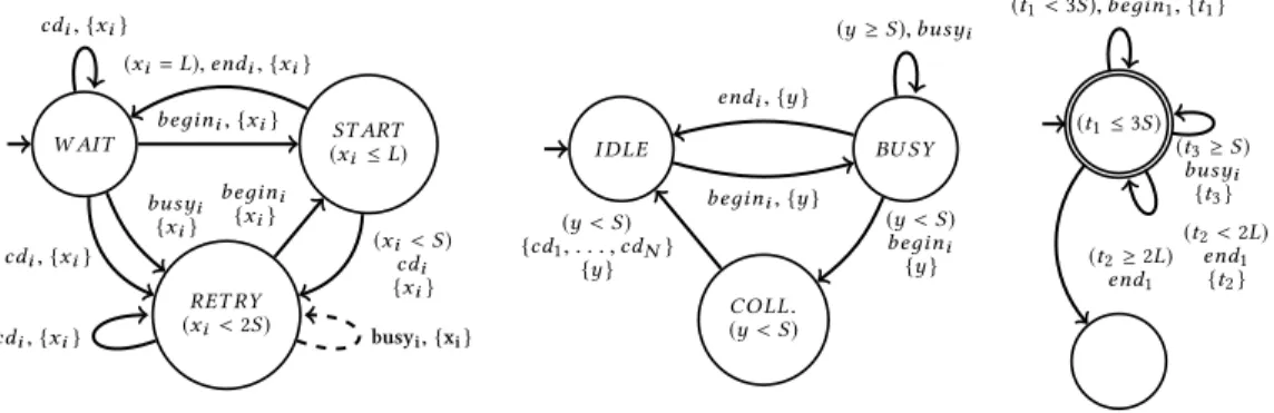
Example 2.3. Figure 1 gives an example of a TBA A1 which has a Büchi accepting run: for

instance the run which leaves state 0 and reaches state 1 at time unit 1, after which the loop transition at state 1 is taken at intervals of 1 time unit. Figure 4 gives a TBA A2for which there is

no Büchi accepting run. The reset ofx and the guard x ≥ 1 imply that between two consecutive

visits to state 1, at least 1 time unit should have elapsed. Sincey is never reset, the value of y keeps increasing by at least 1 unit at each arrival to state 1. Oncey becomes > 100, the guard y ≤ 100 disables the transition from 1 to 0.

The Büchi non-emptiness problem is known to be Pspace-complete [1]. Standard solutions to this problem use regions or zones: they construct an untimed Büchi automaton and check for its emptiness. There are various methods to handle the non-Zeno requirement [9, 17].

Remark 1. In this paper, we will assume that the automata are strongly non-Zeno [15], that is, every infinite accepting run is non-Zeno. It is possible to convert every TBA into a strongly non-Zeno TBA. This strongly non-Zeno construction could lead to an exponential blowup [6, 9] to the abstract zone graph (which is defined below), but we prefer to employ this commonly used assumption in order not to divert from the main subject.

We will now describe a translation which reduces the Büchi non-emptiness problem to checking non-emptiness of an untimed Büchi automaton.

2.2 Abstract zone graphs

As the semantics of a TBA is an infinite transition system, algorithms for TBA consider special sets of valuations called zones. A zone is a set of valuations described by a conjunction of two kinds of constraints: eitherxi ∼c or xi−xj ∼c where xi, xj ∈X , c ∈ Z and ∼∈ {<, ≤, =, >, ≥}.

For example (x1> 3 ∧ x2−x1 ≤ −4) is a zone. Zones can be efficiently represented by Difference

Bound Matrices (DBMs) [5].

The zone graphZG(A) of a TBA A = (Q, q0, X,T, F ) is a directed graph whose nodes are pairs

of the form (q, Z) consisting of a state q of A and a zone Z. The initial node is (q0, Z0) with

Z0 = {0 + δ | δ ∈ R≥0}. For every transitiont = (q,д, R, q′) ∈T , and every set of valuations

W , we define the transition ⇒t _{as: (q,W ) ⇒}t _(q′_,W′

) whereW′ = {v′| ∃v ∈ W , ∃δ ∈ R≥0 :

(q,v) →t_→δ _(q′_,v′_{)}. In other words,W}′_{is obtained by first computing the →}t _{successors ofW ,}

followed by all time successors. It can be shown that ifW is a zone, then so is W′. In the zone graph, from every node (q, Z) there is a transition (q, Z) ⇒t _(q′_{, Z}′

) corresponding to the transitionst fromq. The transition relation ⇒ is the union of ⇒t over allt ∈ T .

Observe that there is a slight difference in the definition of transitions in the automaton (q,v)−−→δ ,t (q′_,v′

) where we first have a delayδ, followed by a transition t, and the definition of transitions in the zone graph: (q,W ) ⇒t _(q′_,W′

) whereW′is the set of valuations obtained fromW by

first taking transitiont, and then doing a delay. The two definitions match since the initial zone encompasses an initial delay from the initial valuation 0.

Although the zone graphZG(A) groups together valuations, the number of zones is still infi-nite [4]. Figure 1 shows an example of a TBA whose zone graph consists of infiinfi-nitely many nodes reachable from the initial node. For effectiveness, zones are further abstracted. Let us write P(S) for the set of subsets ofS. An abstraction operator is a function a : P(R|X |_≥0) → P(R|X |≥0) such that

0 1 y ≤ 100 {x } x ≥ 1 {x } Automaton A1 0, 0= x = y 1, 0 ≤y − x ≤ 100 1, 1 ≤y − x ≤ 101 1, 2 ≤y − x ≤ 102 · · ·

Zone graphZG(A1)

0, 0= x = y 1, 0 ≤y − x ≤ 100 1, 1 ≤y − x ≤ 101 · · · 1, 101 ≤y − x ≤ 201

Abstract zone graphZGa≼LU(A1)

0, 0= x = y 1, 0 ≤y − x ≤ 100 1, 1 ≤y − x ≤ 101

ZGa≼LU(A1) with subsumption

Fig. 1. Example of an automaton whose zone graph is infinite. The abstract zone graph is computed with a_≼LUabstraction, taking L(x)= 1,U (x) = −∞, L(y) = −∞,U (y) = 100. It contains 103 nodes. The zone graph with subsumption contains only 3 nodes. The “squiggly” edge denotes the subsumption: a_≼LU(1 ≤y − x ≤

101) ⊆ a_≼LU(0 ≤y − x ≤ 100).

W ⊆ a(W ) and a(a(W )) = a(W ) for every set of valuations W ∈ P(R|X |≥0). The abstraction is finite

if a has a finite range. An abstraction operator defines an abstract symbolic semantics defined by: (q,W ) ⇒t_a (q′_{, a(W}′_{)) when a(W ) = W and (q,W ) ⇒}t _(q′_,W′_{). Essentially, each time a successor}

W′_{is computed, it is abstracted to a(W}′_{). We define a transition relation ⇒}

ato be the union of ⇒ta

over all transitionst. For a finite abstraction operator a, the abstract zone graph ZGa_{(A) consists of}

node pairs (q,W ) of the form W = a(W ). The initial node is (q0, a(Z0)) where (q0, Z0) is the initial

node ofZG(A). Transitions are given by the ⇒arelation. Such a graphZGa(A) can be seen as a

Büchi automaton with the accepting states (q,W ) for q ∈ F .

2.2.1 The a≼LU abstraction. Abstractions for timed automata are typically parameterized by the

maximum of constants appearing in the guards of the automaton. The structure of the automaton

determines two functionsL : X 7→ N ∪ {−∞} and U : X 7→ N ∪ {−∞}. For a clock x, the value

L(x) denotes the maximum constant occurring in guards of the form x ≥ c or x > c; if no such

guard exists thenL(x) = −∞. The value U (x) denotes the maximum constant occurring in guards

x ≤ c or x < c; if no such guard exists then U (x) = −∞. This can be further refined by considering LU bounds for each state of the automaton [2]. In this paper we will use the abstraction operator a_≼LU [3] and the abstract zone graphZGa≼LU(A) induced by it. Another abstraction operator

Extra+_LU is commonly used in timed automata tools [3]. However, it is known that a≼LU is a coarser

abstraction than Extra+_LU and hence it could potentially lead to smaller abstract zone graphs [3]. We will therefore stick to a≼LU abstraction in this document. In order to define a≼LU, we need to

first define a simulation pre-order on valuations.

Definition 2.4 (LU-preorder [3]). LetL,U : X 7→ N ∪ {−∞} be two bound functions. For a pair of valuations we setv ≼LUv

′

if for every clockx: • ifv′(x) < v(x) then v′(x) > L(x), and • ifv′(x) > v(x) then v(x) > U (x).

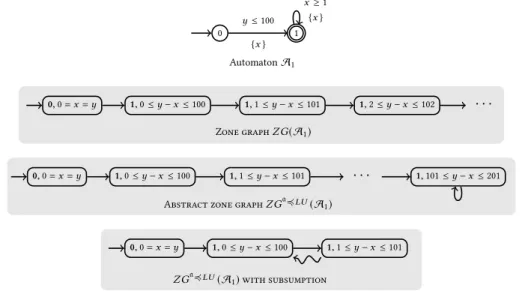
x y U (x) L(x) L(y) U (y) • v′ • u • w • r Z : a≼LU(Z ) : ∪

Fig. 2. The dark gray portion shows a zone Z . The light gray shows the valuations added in the a_≼LU

abstraction of Z , with respect to the LU bounds marked in the picture. Each valuation in the light gray zone is simulated by a valuation in the zone Z w.r.t.≼LU. The abstraction a≼LU(Z) is given by the union of the

shaded portions. The picture illustrates a valuation v′such that r≼LUv′, u≼LUv′and w≼LUv′.

The a≼LUabstraction is based on this relation.

Definition 2.5 (a≼LU-abstraction [3]). GivenL and U bound functions, for a set of valuations W

we define:

a_≼LU(W ) = {v | ∃v

′_{∈W . v ≼}

LUv

′_}.

Figure 2 gives an example of a zoneZ and its abstraction a≼LU(Z). Consider the valuation v

′

in the figure. Note thatU (x) < L(x) < v′(x), and L(y) < v′(y) < U (y). Hence, for a valuation v to be simulated byv′_{, i.e. forv ≼}

LU v′in the definition above, we needU (x) < v(x), and v′(y) ≤ v(y).

We cannot havev′_{(y) > v(y) as this requires v(y) > U (y), that is impossible due to v}′_{(y) < U (y).}

Valuationsr, u and w in the figure satisfy these criteria. In fact, a_≼LU(v′) is the set of valuations

given byx > U (x) and y ≥ v′_(y).

Figures 1 and 4 give examples of abstract zone graphs obtained using a≼LUabstraction. It was

shown in [8] that the a≼LU abstraction induces the smallest zone graphs, for a given bound function

LU . Moreover, we know from [14] that ZGa_{≼LU(A) is sound and complete for Büchi non-emptiness:}

Theorem 2.6. [14] A TBA A has a run satisfying the Büchi condition iff the abstract zone graph ZGa_{≼LU(A) has a run satisfying the Büchi condition.}

This gives an algorithm for the Büchi non-emptiness problem: given a TBA A, compute the (finite) Büchi automatonZGa≼LU_{(A) and check for its emptiness. There is however a challenge due}

to the use of the a_≼LUabstraction. There are zonesZ for which a≼LU(Z) is non-convex (c.f. Figure 2)

and hence it is better to avoid storing a_≼LU(Z). Therefore, the solution to compute ZGa≼LU(A)

works with a graph consisting of (state, zone) pairs and uses the a_≼LUabstraction indirectly [8]. The

algorithm for computingZGa_{≼LU(A) is shown in Figure 3. We will denote the transition relation}

⇒ by → for convenience, as shown by the edge relation in Figure 3.

We now state a lemma which makes the optimization described in the next section possible.

Lemma 2.7 (Simulation property of a_≼LU-abstraction). Let A be a TBA, andLU be bound

functions computed from guards of A. For every pair of nodes (q, Z) and (q, Z′_{) ofZG}a_{≼LU(A): if}

a_≼LU(Z) ⊆ a≼LU(Z′), then for every transition (q, Z) → (q1, Z1), there exists (q, Z′) → (q1, Z₁′) such

that a≼LU(Z1) ⊆ a≼LU(Z₁′).

We refer the reader to [3] and [12] for a proof of the above lemma, and a more detailed account of the a_≼LUabstraction (both of which are not required for the rest of this paper). We however present

a brief intuition about why this property holds. Roughly, we want a relation between valuationsv andv′_{which ensures that wheneverv satisfies a guard д, valuation v}′_{also satisfiesд (and hence}

1 procedure_{abstract_zone_graph(A)}

2 V := {(q0, Z0)}, Waiting := {(q0, Z0)} 3 → := ∅ // edge relation

4 while_{(Waiting , ∅)}

5 take and remove (q, Z ) from Waiting 6 for eacht = (q, д, R, q′) ∈ A

7 compute (q, Z ) ⇒t(q′, Z′)

8 if∃(q′, Z₁) ∈V s.t a_≼LU(Z′)= a_≼LU(Z₁)

9 add(q, Z ) → (q′, Z₁)

10 else

11 add(q′, Z′_{) to}V and Waiting

12 add(q, Z ) → (q′, Z′) 13 return(V , →) 14 15 16 17 18 19 procedure_{subsumption_graph(A)} 20 V := {(q0, Z0)}, Waiting := {(q0, Z0)} 21 → := ∅ // edge relation 22 ⇝ := ∅ // subsumption relation 23 while(Waiting , ∅)

24 take and remove (q, Z ) from Waiting 25 for eacht = (q, д, R, q′) ∈ A 26 compute (q, Z ) ⇒t(q′_{, Z}′₎ 27 if∃(q′, Z₁) ∈V s.t a_≼LU(Z′)= a_≼LU(Z₁) 28 add(q, Z ) → (q′, Z₁) 29 else if∃(q′, Z₁) ∈V s.t. a_≼LU(Z′_{) ⊆ a} ≼LU(Z1) 30 add(q′, Z′) toV 31 add(q, Z ) → (q′, Z′) and (q′, Z′) ⇝ (q′, Z₁) 32 else

33 add(q′, Z′) toV and Waiting

34 add(q, Z ) → (q′, Z′)

35 return(V , →, ⇝)

Fig. 3. Algorithm on the left computes ZGa≼LU_{(A). The test a}

≼LU(Z

′_{)= a}

≼LU(Z1) can be done using the

method in [8]. On the right is an algorithm which uses subsumption.

runs fromv can be simulated by runs from v′). TheLU bound functions say that all lower bound guardsx ≥ c, x > c have c ≤ L(x) and all upper bound guards x ≤ c, x < c have c ≤ U (x). Hence, whenv′_{(x) < v(x), a problem arises when a lower bound guard д is of the form x ≥ c or x > c}

withv′_{(x) ≤ c ≤ v(x) as this will lead to v satisfying д, but v}′_{violatingд; in this case v}′_cannot

simulatev. This motivates the first condition in the definition: if v′_{(x) < v(x) then v}′_{(x) > L(x).}

Similar reasoning holds for the symmetric case.

For a noden ∈ ZGa_{≼LU(A) we writen.q and n.Z for the state and zone present in node n}

respectively.

2.3 Using subsumption to compute smaller graphs

AlthoughZGa_{≼LU(A) is the smallest abstract zone graph for a givenLU , its size could be (and}

usually is) exponential in the size of A. An essential optimization that makes analysis of timed automata feasible is the use of subsumption. For two nodest and s of ZGa_{≼LU(A) we sayt is}

subsumed bys, written as t ⊑ s, if t.q = s.q and a≼LU(t.Z) ⊆ a≼LU(s.Z). When t ⊑ s, the node

s simulates t. Hence, at least for testing reachability, it is enough to keep in the graph only the maximal nodes with respect to subsumption. The algorithm incorporating subsumption is shown in the right hand side of Figure 3.

Subsumption optimization is known to give substantial gains for the reachability problem [11]. However, subsumption is not a priori correct for liveness: in Figure 1, the zone graph with subsump-tion contains no cycle consisting entirely of → edges but the zone graph has one. Admitting cycles with subsumption edges is not sound either: Figure 4 illustrates an example of an automaton whose zone graph has no cycles, but zone graph with subsumption has a cycle consisting of → and ⇝ edges. Therefore, it is not immediately clear how to decide Büchi non-emptiness from subsumption graphs (in other words, zone graphs with subsumption edges). The question of how subsumption graphs can be used for Büchi non-emptiness was raised in [15]. An algorithm proposed in [13]

0 1 y ≤ 100 x ≥ 1, {x }

Automaton A2

0, 0= y − x 1, 1 ≤y − x 0, 1 ≤y − x ≤ 100 1, 2 ≤y − x ≤ 101 · · · 1, 101 ≤y − x

Abstract Zone graphZG(A2)

0, 0= x = y 1, 1 ≤y − x 0, 1 ≤y − x ≤ 100

ZGa≼LU(A₂) with subsumption

Fig. 4. Example of an automaton with no Büchi accepting run. Abstract zone graph is computed with L(x)= 1,U (x) = −∞, L(y) = −∞,U (y) = 100. There are no cycles in abstract zone graph. Allowing subsumption gives a smaller graph. However the graph with subsumption has an infinite path that does not correspond to any run of A2. In general, counting subsumption edge as part of cycles is incorrect for Büchi emptiness.

1 procedure_ndfs()

2 Cyan := Blue := Red := ∅

3 dfsBlue(s₀) 4 reportno cycle 5 6 proceduredfsRed(s) 7 Red := Red ∪ {s } 8 for alls → t do

9 if(Cyan ⊑ t ) then report cycle

10 if(t ̸⊑ Red) then dfsRed(t )

11

12 proceduredfsBlue(s)

13 Cyan := Cyan ∪ {s } 14 for alls → t do

15 if(t < Blue ∪ Cyan and t ̸⊑ Red)

16 thendfsBlue(t )

17 if(s ∈ F ) then

18 dfsRed(s) 19 Blue := Blue ∪ {s } 20 Cyan := Cyan \{s }

Fig. 5. Nested DFS algorithm with subsumption [13] to compute a subgraph of ZGa≼LU_(A)

(illustrated in Figure 5) gives a restricted way of using subsumption in a nested DFS algorithm for detecting accepting cycles. It exploits the following property: if we know that from a node s there is no reachable accepting cycle, then no node t ⊑ s needs to be explored. The red nodes in the nested DFS algorithm play the role of nodes (c.f. Lines 10 and 15 in algorithm). Another optimization occurs in Line 9 - if there is a path from a nodet to node s subsuming it, then a cycle can be concluded.

The goal of this paper is to find subsumption graphs ofZGa≼LU_{(A) that are sound and complete}

for liveness, and to design efficient algorithms to compute them.

3 LIVENESS COMPATIBLE SUBSUMPTIONS

In this section, we are interested in understanding generic conditions for subsumption to be correct for liveness analysis. We start with an example. Consider the TBA A3andZGa≼LU(A3) illustrated

q r s t Automaton A3 {x } {x } x ≥ 1 {x } y ≤ 100 x ≥ 1 {x } (q, x = y ≥ 0) (r , 0 ≤ y − x) (r , 1 ≤ y − x) (r , 2 ≤ y − x) (r , 100 ≤ y − x) (r , 101 ≤ y − x) (s, 0 ≤ y − x) (t , 0 ≤ y − x ≤ 100) (s, 1 ≤ y − x ≤ 101) (t , 1 ≤ y − x ≤ 100) (t , y − x = 100) (s, y − x = 101) .. . .. .

Fig. 6. On the left is a TBA A3; on the right the graph obtained by removing the two squiggly edges is

ZGa_≼LU(A

3). Assume that L= U = 100 at every state. This can be achieved by adding more transitions on

each state (which are not shown for clarity). Squiggly edges show subsumptions. The part of ZGa≼LU_(A3)

restricted to white nodes and squiggly edges is the zone graph with subsumption. In this graph there is no accepting cycle consisting only of → edges. Removing the squiggly edge on the node (r, 1 ≤ y − x) and adding the grey nodes having state r identifies the accepting cycle.

an accepting cycle on the node (r, 101 ≤ y − x). For each of the states r, s and t of the TBA, there are at least 100 nodes in the zone graph. Note that (r, 1 ≤ y − x) ⊑ (r, 0 ≤ y − x) and (s, 1 ≤ y − x ≤ 101) ⊑ (s, 0 ≤ y − x). If we allowed the luxury to use subsumptions freely, we would get the graph consisting only of the white nodes in the figure and the two squiggly edges denoting subsumption. However, in this graph there is no accepting cycle made uniquely of → edges. There are cycles containing subsumption edges but, as we have seen in Figure 4, it is not sound to take such cycles as witnesses for the existence of an accepting computation in general. Hence, the subsumption on (r, 1 ≤ y − x) should not be used to detect accepting cycles. On the other hand, the graph of white nodes with no subsumption edge is not complete for liveness as it has no accepting run. Observe that using subsumption on the node (s, 1 ≤ y − x ≤ 101) would do no harm, as further exploration would not lead to accepting cycles anyway. This subsumption gives already a significant gain. In fact, the zone graph restricted to the white and grey nodes, along with the subsumption edge on the right is a liveness complete graph according to our definition below. Algorithm in Figure 5 does not detect this possibility and explores the whole graph.

Our goal is to make use of subsumption as much as possible, subject to the restriction that the resulting graph contains an accepting cycle of → edges iffZGa≼LU_{(A) contains one. Since including}

subsumption edges as part of a cycle is not sound in general, we will avoid using subsumption edges in cycles that contain accepting states. Therefore, in the graphs that we construct, cycles with accepting states will be actual cycles inZGa≼LU_{(A) - so every such cycle will give an accepting}

computation. The challenge is to decide what are the subsumptions that are safe and can be left in the graph. We first make precise the notion of a graph with subsumptions, and then follow up with a condition that makes a zone graph with subsumption complete for liveness.

Definition 3.1 (Subsumption graph). LetG be a graph consisting of a subset of nodes and edges of ZGa_{≼LU(A) together with new edges called subsumption edges. Each node is labeled either covered}

or uncovered. Such a graph is called a subsumption graph if it satisfies the following conditions: C1 the initial node ofZGa≼LU_{(A) belongs to}G and is labeled uncovered,

C2 for every uncovered nodes, all its successor transitions s −→s′occurring inZGa≼LU_(A)

C3 for every covered nodet ∈ G there is an uncovered node s ∈ G such that t ⊑ s; moreover there is an explicit subsumption edget ⇝ s in G,

C4 there is a path of −→ edges from the initial node to every other node.

A path in a subsumption graph is made of both → and ⇝ edges. We write s1d∗s2to denote

that there is a path froms1tos2in the subsumption graph. We now describe the relation between

paths in a zone graph and in a subsumption graph. For the rest of this section, we fix an automaton

A and a subsumption graphG for A.

Lemma 3.2. For every (finite or infinite) paths0→s1→s2→ · · · inZGa≼LU(A) there is a path

s′ 0d ∗_s′ 1 d ∗_s′ 2d ∗

· · · inG such that for each i, si ⊑s_i′ands_i′is uncovered.

Proof. Proof proceeds by induction. From C1, the initial nodes0is present inG and is uncovered.

Suppose we have constructeds₀′ d∗s1′ d ∗ _{· · ·s}′

n. Sincesn ⊑s_n′, there is a transitions_n′ →s_n+1′ such thatsn+1⊑s_n+1′ inZGa≼LU_{(A) (c.f. Lemma 2.7). As}s′

n is uncovered, this transition is present

inG (C2). If s_n+1′ is uncovered inG, we are done. Otherwise, there is an edge s_n+1′ ⇝ sn+1′′ inG with

s′

n+1⊑sn+1′′ (C3). This givessn′ d∗s_n+1′′ as required. □

Lemma 3.2 along with condition C4 says that if there is a paths0→∗s in ZGa≼LU(A), there is a

paths0→∗s′withs ⊑ s′in the subsumption graphG. This shows that subsumption graphs are

complete for reachability. However, these conditions are not sufficient for liveness - for a cycle of → edges in the zone graph, we may not get a corresponding cycle of → edges in the subsumption graph (c.f. Figures 4 and 6). We now give an extra criterion.

Definition 3.3 (Liveness compatible subsumption graph). A subsumption graphG is said to be

liveness compatible if it additionally satisfies the following condition:

C5 there is no cycle containing both an accepting node and a subsumption edge.

In Figure 6, the zone graph restricted to white nodes and the squiggly edges is not liveness compatible. There is a cycle containing an accepting node (r, 1 ≤ y − x) and a subsumption edge from this node. However, removing this subsumption edge and adding the grey nodes makes it liveness compatible. The only remaining subsumption edge is from (s, 1 ≤ y − x ≤ 101) and it is not part of a cycle containing an accepting node. Intuitively, when we add a subsumption edget′

⇝ s′_,

we know that paths inZGa_{≼LU(A) starting fromt}′

can be simulated froms′in the subsumption graph. But if there is a cycle containingt′⇝ s′in the subsumption graph, this would mean that the simulation froms′can bring us back tot′. Hence some accepting runs fromt′inZGa≼LU_(A)

could be lost in the subsumption graph. We show that condition C5 above makes such a situation impossible.

Theorem 3.4. ZGa_{≼LU(A) has an infinite accepting path iff a liveness compatible subsumption}

graph has an infinite accepting path consisting of → edges.

Proof. LetG be a liveness compatible subsumption graph. Since all the −→ edges inG come

from the zone graph, a cycle of −→ edges inG implies such a cycle in the zone graph. This shows the direction from right to left. SupposeZGa_{≼LU(A) has an accepting runρ: s}

0→− s1→ · · · . From−

Lemma 3.2, we have a pathρ′inG of the form: s₀′ d∗s1′ d ∗ _s′

2 d ∗

· · · such that eachsi ⊑s_i′. Sinceρ is an accepting run, some accepting node s repeats infinitely often in ρ. Corresponding positions inρ′contain nodes which subsumes. Since there are finitely many nodes in G, there should be some accepting nodes′which occurs infinitely often inρ′. Therefore there is a cycle containings′inG. By liveness compatibility criterion C5 this cycle should be made of only −→ edges. From condition C4, there should be a path consisting of −→ edges from the initial node ofG

tills′_{. This gives an infinite path inG made of → edges that visits an accepting node s}′_infinitely

often. □

The above theorem gives a characterization for the use of subsumption to decide liveness. It now remains to design an algorithm that computes such graphs. Before we give an algorithm, we make an observation about the complexity of computing liveness compatible subsumption graphs. Note that these liveness compatible subsumption graphs have more nodes than subsumption graphs used for reachability. In the next section, we show that liveness compatible graphs can be much larger than subsumption graphs, and there is an intrinsic difficulty in inferring liveness from plain subsumption graphs (which are sound and complete for reachability).

4 DECIDING LIVENESS FROM SUBSUMPTION GRAPHS IS PSPACE-COMPLETE

In order to understand the overhead created due to the liveness compatibility condition, we consider a variant of the non-emptiness problem for TBA (Definition 2.2) where a subsumption graph of

the automaton is also given as input. A subsumption graphG of a TBA A is minimal if for every

two nodess and t, if s ⊑ t then s = t or s is the initial node of ZGa≼LU_{(A). In other words,}G only

contains incomparable nodes w.r.t. ⊑, except for the initial node that may not be maximal inG

w.r.t. ⊑. We show that the emptiness problem for TBA remains Pspace-complete even withG as

the input. This contrasts with the reachability problem that can be solved in polynomial time from G. We first formalize the problem under consideration. The Büchi non-emptiness problem with subsumption graph (EMPTY-SUB) is defined by:

INP UT:A TBA A and a minimal subsumption graphG for A

OUTP UT: “Yes” if A has a Büchi accepting run, “No” otherwise.

Theorem 4.1. The problem EMPTY-SUB is Pspace-complete.

The upper bound follows since determining Büchi non-emptiness from the automaton can be done in Pspace. For the Pspace-hardness, we give a reduction from the membership problem for Linear Bounded Automata (LBA). Recall that an LBA is a Turing machine whose tape is restricted to the part on which the input word is written. The membership problem for LBAs asks whether the accepting state is reachable from the initial state and initial tape contentw. This problem is known to be Pspace-complete, even for deterministic LBAs over a binary alphabet. Without loss of generality, we consider a deterministic LBA B, over the binary alphabet {0, 1} with initial tape contentw ∈ {0, 1}N, and hence tape of sizeN . We describe a construction of a TBA AB,w such that:

(1) it has a Büchi accepting run iff B has an accepting run starting withw on the tape; (2) AB,w has a unique minimal subsumption graphG which has size polynomial w.r.t. the size

of B andw;

(3) there is a polynomial time algorithm that given B andw, constructs AB,w andG.

This gives a polynomial-time reduction from the membership problem of LBAs to EMPTY-SUB, thus proving Theorem 4.1.

We proceed in two steps: first we describe a TBA A_B,w′ which satisfies requirement 1 given above; following this, to satisfy requirement 2, we make some modifications to A′

B,w to get the

final automaton AB,w.

4.1 Building TBA A′_B,w that simulates the LBA

The main point is to encode the tape of B. Each celli ∈ [1; N ] of the tape is represented in A_B,w′ by a clockxi such thatxi = 2i when cell i contains a 0, and xi = 2i + 1 when it contains a 1. To

simplify the construction, we introduce an extra clocky. We let X = {x1, . . . , xN, y} denote the

set of clocks of A′

B,w. A clock valuationv encodes a tape content w ∈ {0, 1}N whenv(y) = 0 and

v(xi)= 2i + wifor everyi ∈ [1; N ] (where wi denotes the content of theithcell). We write enc(w) for the valuation that encodesw.

For every stateq of B, we have a state qi, ·,N in A′_B,w wherei ∈ [1; N ] encodes the position of the tape head. The transitions of B are encoded by sequences of transitions in A′_B,w. We introduce intermediate states in A′_B,w of the formqi,t ,k whereq is a state in B, i ∈ [1; N ] is the position of the tape head,t is the transition in B that is simulated in A′

B,w, andk ∈ [0; N ] is an index

pointing to a cell that is being processed in our simulation. Lett be a transition q−−−−→α ,β ,∆ q′in B withα, β ∈ {0, 1} and ∆ ∈ {−1, 0, 1}: when B is at q and the tape head points to a cell with letter α, the LBA overwrites it withβ, moves the tape head according to ∆ and changes its state to q′. This transitiont is simulated by the following sequence in A′_B,w:

qi, ·,N (y=0)∧(xi=2i+α) −−−−−−−−−−−−−→qi,t ,N −x−−−−−−−−N=2(N +1)→ {xN} qi,t ,N −1−−−−−−−−−−→xN −1=2(N +1) {xN −1} · · · · · ·qi,t ,i −−−−−−−−−−−−−xi=2(N +1)+α−β→ {xi} · · · (1) · · ·qi,t ,1−−−−−−−−→x1=2(N +1) {x1} qi,t ,0−−−−−−−→y=2(N +1) {y } q ′ i+∆,·,N

Except for the names of the states, the only elements in (1) parameterized byt and i are the guard of the first transitionxi = 2i + α and the guard from the middle transition xi = 2(N + 1) + α − β. In

particular, all sequences have the same last transition that checksy = 2(N + 1) and that resets y. Clocky ensures that the duration of sequence (1) is exactly 2(N + 1), and that time does not elapse in states of the formqi, ·,N thanks to the first guardy = 0.

The first transition checks that celli contains α by testing if xi = 2i + α. Then, subsequent

transitions simulate a sequential access to the tape, from its last cell, encoded byxn, to its first cell,

encoded byx1. The value of any clockxj , xi is left unchanged by (1). Indeed, ifv is the value of

xj inqi, ·,N, then 2(N + 1) − v time units must elapse before the transition

xj=2(N +1)

−−−−−−−−→

{xj}

is taken, and v time units elapse after the transition since the total delay on the sequence is 2(N + 1). Hence xj = v in q_i+∆,·,N′ . The transition−x−−−−−−−−−−−−i=2(N +1)+α−β→

{xi}

updates the value of the clockxi. Due to the first

transition in the sequence, we know thatxi = 2i + α in qi, ·,N. Then, 2(N + 1) − (2i + β) time units

elapse before the transition is taken, and we delay 2i + β after this transition to reach a total delay of 2(N + 1) along the sequence. Hence xi = 2i + β in q_i+∆,·,N′ , thereby encoding the new valueβ of

celli. Observe that every transition on (1), except the first one, is enabled since for every k ∈ [1; N ], xk ≤ 2N + 1 when qi,t ,k is reached, andy ≤ 2N + 1 when qi,t ,0is reached. Finally, the automaton reaches stateq_i+∆,·,N′ hence simulating a move to stateq′with tape head on celli + ∆ in B.

A′

B,w has an initialisation sequence that encodes the initial wordw in the clocks:

q_{1, ·,N} xN=2+(wN−wN −1) −−−−−−−−−−−−−−−→ {xN −1} · · ·q_{1, ·,i} −−−−−−−−−−−−→xi=2+(wi−wi −1) {xi −1} q_{1, ·,i−1}· · ·q_{1, ·,1}−−−−−−−x1=2+w→1 {y } q 0 1, ·,N (2)

whereq0_{is the initial state of B andq}

1, ·,k are new intermediate states withk ∈ [1; N ] and q is

distinct from all states in B. Starting with all clocks equal to 0, the automaton reachesq0_{1, ·,N} with y = 0 and xi = 2i + wi for alli ∈ [1; N ], hence valuation enc(w).

A configuration of B is a triple (q, i,u) where q is a state of B, i ∈ [1; N ] is the position of the tape head, andu ∈ {0, 1}N is the content of the tape. From the construction above, we get that LBAs can be simulated by TBAs:

Lemma 4.2. A configuration (q, i,u) is reachable in an LBA B started on an input word w if and only if the configuration (qi, ·,N, enc(u)) is reachable in A′_B,w from the initial stateq_{1, ·,N}.

The above lemma talks only about reachability while requirement 1 above talks about a Büchi run. The last step in our construction of A′_B,w is to cater to this. Without loss of generality, we can assume that B has a unique accepting stateqf with no outgoing transition. We make every state of the formqf_{i, ·,N} withi ∈ [1; N ] as accepting in A′_B,w. For every tape head positioni ∈ [1; n], we add an extra edge:

qf_{i, ·,N} −−−−−−−−−−−→

{x1, ··· ,xN,y }

q1, ·,N (3)

that restarts A′_B,w in its initial configuration once an accepting state has been reached. From Lemma 4.2 we get that:

Corollary 4.3. B has a finite accepting run on input wordw iff A′_B,w has a Büchi accepting run with initial stateq_{1, ·,N}.

4.2 Small Subsumption Graph for A′

B,w

A crucial point for our proof of Theorem 4.1 is to get a small minimal subsumption graphG for

A′

B,w. More precisely the size ofG should be polynomial w.r.t. the size of B and w. To get this, we

will add some states and edges to A′_B,w.

A clock order is a total order on the setX of clocks of A′_B,w. Leti be an integer between 0 and N . We denote ⊴i the clock orderxi+1⊴i · · · ⊴i xN ⊴iy ⊴i x1⊴i · · · ⊴i xi. A valuationv satisfies a

clock order ⊴i if for all clocksz, z′∈X we have v(z) ≤ v(z′) ⇔z ⊴i z′. A setS of clock valuations

satisfies ⊴i if all clock valuationsv ∈ S satisfy ⊴i. Sequences (1) and (2), reset the clocks in the

same order: firstxN, thenxN −1, . . . , thenx1, and finallyy. The initial clock valuation, where all

clocks have value 0, obviously satisfies ⊴N. Then, by construction of A′

B,w, we get that:

Lemma 4.4. For every configuration (qi,t ,k,v) reachable in A′_B,w from the initial stateq_{1, ·,N}, the valuationv satisfies ⊴k.

All the reachable zones in the (unabstracted) zone graph of A′

B,w are sets of reachable valuations.

Hence, from Lemma 4.4, we have that in every reachable node (qi,t ,k, Z) in the zone graph of A′B,w,

Z satisfies ⊴k. We now use this observation to modify A′_B,w to get a small minimal subsumption graph. LetZ⊴k = {v ∈ R

N +1

≥0 |v satisfies ⊴k} be the set of valuations that satisfy ⊴k. Observe that

Z⊴k is a zone. The next step of the construction consists in modifying A

′

B,w in such a way that its

zone graph contains nodes (qi,t ,k, Z⊴k) for every stateqi,t ,k in the automaton. From Lemma 4.4,

these zones are maximal w.r.t. zone inclusion, and subsume every other reachable zone. This way we will ensure that (1) the minimal subsumption graph is unique, and (2) it does not depend on A′

B,w, except for the names of states, and from this we will get an easy bound on its size.

We add a new initial stateι, and sequences from ι producing the zones Z_⊴k. For allk, j ∈ [0; N ], we introduce intermediate statesιk,j and transitions:

ι −−−−→ {xk} ιk,N· · · −−−→ {x1} ι_{k,N −k+1}−−−→ {y } ιk,N −k −−−−→{xN} · · ·ι_k,1−−−−−→ {xk+1} ιk,0 (4)

Starting fromι, every valuation obtained in ιk,0satisfies ⊴k. Moreover, the zone that is reachable

these sequences to all relevant states of A′

B,w with the effect that every state is reachable with a

maximal zone:

ιN ,0→qi, ·,N for everyi ∈ [1; N ] (5) ιk,0→qi,t ,k for everyi ∈ [1; N ], t ∈ T, k ∈ [0; N ] (6) ιk,0→q1, ·,k for everyk ∈ [1; N ] (7)

We are now ready to formally define AB,w.

Definition 4.5. Let B be a deterministic LBA (Q, q0, qf, {0, 1},T, N ) such that the accepting state

qf has no outgoing transitions. Letw ∈ {0, 1}N be an initial tape content of B of lengthN ≥ 0. We

define the TBA AB,w = (S, ι, F, X, →) by:

• S = {qi, ·,N |q ∈ Q, i ∈ [1; N ]} ∪ {qi,t ,k|q ∈ Q, i ∈ [1; N ], t ∈ T, k ∈ [0; N ]} ∪ {q_{1, ·,k}|k ∈ [1;N ]} ∪ {ι} ∪ {ιi,k|i, k ∈ [0; N ]} is the set of states,

• ι ∈ Q is the initial state,

• F = {qf_{i, ·,N} |i ∈ [1; N ]} is the set of final states, • X = {x1, . . . , xN, y} is the set of clocks,

• → is the transition relation defined by:

– for every transitiont ∈ T and every tape head position i ∈ [1; N ], there are simulation transitions as in (1);

– there are initialisation transitions as in sequence (2);

– for every tape head positioni ∈ [1; N ], there is a restart transition (3); – for everyk ∈ [0; N ], there are reset sequences as (4);

– and for everyi ∈ [1; N ], every t ∈ T , and every k ∈ [0; N ] there are maximal zone

transitions as in (5), (6), and (7).

We first state the reduction of the membership problem for Linear Bounded Automata to the emptiness for Timed Büchi Automata.

Lemma 4.6. A deterministic LBA B accepts a wordw iff AB,w has a Büchi accepting run. This result follows from Corollary 4.3. Observe that on an accepting Büchi run, A′_B,w visits an accepting state infinitely many times. Each time it enters an accepting state it is re-initialised. In A_B,wthe first part of the run may be perturbed because of maximal zone generation sequences (4), (5), (6) and (7). Nevertheless, after reaching an accepting state for the first time, the state of, AB,w

is reset and it works the same way as A′ B,w.

As a result of adding sequences (4), (5), (6) and (7) that first generate maximal zones, the minimal subsumption graph for AB,w is small.

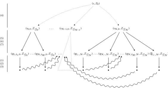
Lemma 4.7. Let B be an LBA,w be a word over {0, 1} and let AB,w be the corresponding LBA. The automaton AB,w and its minimal subsumption graph have a size polynomial in the size of B andw. Proof. Observe from Definition 4.5 that AB,w is itself of size polynomial in the size of B andw. LetG be the minimal subsumption graph for AB,w. We show that it is linear in the size of AB,w. The bound on the size ofG follows from the observation that there is at most one node in G for every state in AB,w. This can be seen from Figure 7. The statesι and ιk,jwithk, j ∈ [0; N ] can only be reached once following sequences (4). Now, transitions (5), (6) and (7) generate zonesZ⊴N for

statesqi, ·,N, andZ⊴k for statesqi,t ,k andq1, ·,k. Taking one more transition from these nodes by

following sequences (1), (2) or (3) yield new nodes which are covered by the maximal zonesZ⊴i at

(ι, Z0) (ι0,0, Z_⊴0) . . . (ι_{N −1,0}, Z_{⊴N −1}) (ι_{N ,0}, Z_⊴N) (q_1,t1,0, Z_⊴0) . . . (q_{N ,tM ,0}, Z_⊴0) . . . (q_{1,·, N}, Z_⊴N). . . (q_{N ,·, N}, Z_⊴N) . . . (q_{N ,tM ,N}, Z_⊴N) (q_{1,·, N}, Z_⊴N) • • • • • • (4) (5) (6) (7) (1) (2) (3)

Fig. 7. The minimal subsumption graph for AB,w. The first level depicted as dotted lines represents the sequences of transitions and nodes corresponding to (4). The second level are the nodes generated by transitions (5), (6) and (7). The third level are nodes generated by one transition of (1), (2) and (3). The nodes reached after these transitions, denoted • in the picture, are subsummed by the nodes at the previous level, as shown by the squiggly edges.

4.3 Polynomial-time reduction for EMPTY-SUB

To finish the proof of Theorem 4.1, it remains to show that requirement 3 is satisfied by our

construction: namely, the minimal subsumption graph of AB,w can be computed in polynomial

time. Let us recall what we have done till now. Given an LBA B and an input wordw, we have

shown how to construct in polynomial time automaton AB,w. Lemma 4.7 shows that the minimal

subsumption graphG for AB,w has polynomial size. To constructG in polynomial time we can

simply run a breadth-first search on the unabstracted zone graphZG(AB,w) as illustrated in

Figure 7. Starting from (ι, Z0) whereZ0is the zone consisting of valuations in which all clocks are

equal, one follows sequences (4). From the structure of AB,w, this computes all nodes (ικ,0, Z⊴k).

In the next step following transitions (5), (6) and (7), all states of A′_B,w will be visited along with their maximal zonesZ⊴i. Therefore, at depthN + 2, the BFS generates exactly one node for each

state in AB,w containing the associated maximal zone. This takes polynomial time since up to

depthN + 1 the automaton consists just of a linear number of sequences as in (5), (6), and (7). Then, due to subsumption, BFS stops at depthN + 3 after one transition from (1), (2) or (3). The number of nodes at levelN + 3 is bounded by the maximal out degree of the states in AB,w times the number of nodes inG. This is again of polynomial size w.r.t. B and w. Hence we get:

Lemma 4.8. There is a polynomial time algorithm constructing the minimal subsumption graph of AB,w when given B andw.

Initial Subsumption graph

SCC analysis:

IdentifyUnsafeand Safe SCCs Remove subsumptions from nodes within unsafe SCCs

Extend graph: New subsumptions only to safe or fresh nodes (squiggly edges)

Accepting cycle or no unsafe SCC

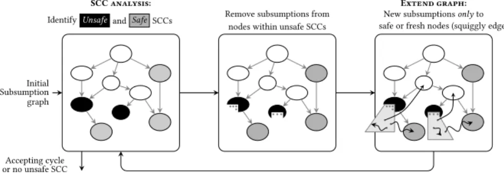
Fig. 8. Illustration of the iterative algorithm to construct liveness compatible subsumption graphs.

5 A NEW ALGORITHM FOR LIVENESS

We now consider the algorithmic problem of computing a liveness compatible subsumption graph for a given automaton. Section 3 says that such a graph allows us to determine if the automaton has a Büchi run. Section 4 indicated that computing such a graph may be much more complex than just computing the subsumption graph using the algorithm in the right of Figure 3. The objective is of course to compute a small graph, as otherwise we could just compute the entire abstract zone graph without subsumption using the algorithm from the left of Figure 3. A better solution is the nested DFS algorithm in Figure 5 - indeed the final graph computed by it is a liveness compatible subsumption graph. In this section, we present a different algorithm, and compare its performance with the nested DFS approach. Our algorithm iterates between a reachability computation and an SCC analysis of the computed graph to find cycles violating condition C5 in Definition 3.3. Recall that a cycle violates C5 if it contains both an accepting state and a subsumption edge; we will call such cycles unsafe in the rest of this section.

Figure 8 illustrates the idea of the algorithm. It starts with an initial subsumption graph obtained by a reachability analysis. This subsumption graph may potentially contain unsafe cycles. The algorithm proceeds by performing an SCC decomposition of the graph by considering → ∪ ⇝ as the edge relation (shown by the left figure, with each bubble denoting an SCC). An SCC is marked Unsafe (black bubble) if it contains an accepting state and a subsumption edge (with both ends in the same SCC). An SCC is marked Safe (grey bubble) if it cannot reach an unsafe SCC. If an accepting cycle (consisting only of → edges) is found during this analysis, the algorithm terminates saying that the automaton has a Büchi accepting run. Otherwise, the algorithm proceeds to the next step. The SCC analysis guarantees that the grey part is liveness compatible and exploration-complete, whereas the remaining part is not yet liveness compatible. Subsumption edges from nodes within unsafe SCCs are removed. This opens nodes for exploration (shown in the middle picture as dots in the black bubbles). A subsumption graph construction is started from the grey dots with subsumption restricted to the previously found safe nodes or the fresh nodes which appear in the new exploration (shown by the squiggly edges in the picture on the right). This restriction is imposed in order to avoid falling repeatedly into the same bad cycle: the grey nodes were subsumed by nodes in their inhabiting black SCCs, and hence the successors of grey nodes will also be subsumed by the corresponding successors in the black SCCs. So such subsumptions would stop the new exploration in one step. Even with this restricted subsumption, it is still possible that new unsafe cycles are formed. Therefore, once the new exploration terminates, the obtained subsumption graph is passed on for the SCC analysis. This process is iterated till either the SCC analysis identifies an accepting cycle, or there are no more unsafe SCCs. The latter case gives a

liveness compatible subsumption graph with no accepting cycles and hence the algorithm can terminate saying that the automaton has no Büchi run. The algorithm needs to handle an extra detail: the removal of subsumption edges after the SCC analysis could lead to dangling nodes that are not → reachable from the initial node. All such nodes are removed before the next subsumption graph computation (in the picture on the right).

The algorithm can be viewed as an iterative refinement of the initial subsumption graph till a liveness compatible graph is obtained. To achieve the behavior of restricted subsumption, a level field is added to each node and subsumption is allowed only between nodes of the same level, or to nodes in the previous levels that do not reach unsafe cycles (nodes in grey SCCs).

We will now give a more detailed description of the algorithm. We will say that a nodes is

covered if it has an outgoing subsumption edges ⇝ s′, for somes′, otherwises is uncovered. Iterative SCC based algorithm with subsumption:

Phase 0 (Initialize). LetS_init andS be the singleton sets containing the initial node which is the initial (state, zone) pair. Set the level of this node to 1. LetK = 1.

Phase 1 (Construct levelK subsumption graph). Construct a subsumption graph from nodes

inSinit in the following manner. Set the pool of nodes to be explored to be equal toSinit. Every node added in this phase will have level field set toK. Repeatedly, pick a node (q, Z) from the pool (and remove it from the pool). For every edge (q, Z) ⇒ (q′_{, Z}′_{), check if there}

is already a node (q′_{, Z}

1) ∈S for which one of the conditions below holds:

1.1 a_≼LU(Z′)= a_≼LU(Z₁), or

1.2 a_≼LU(Z′) ⊂ a_≼LU(Z₁), node (q′, Z₁) is uncovered and has the levelK or ∞. If there is no such node, then add the node (q′_{, Z}′

) to the pool as well as toS, and add the edge (q, Z) → (q′_{, Z}′

) toS. Moreover, for every uncovered (and not initial) node (q′, Z2) of

levelK with a≼LU(Z2) ⊂ a≼LU(Z

′_{): add (q}′_{, Z}

2) ⇝ (q′, Z′) and remove all other edges from

(q′_{, Z} 2).

If there is (q′_{, Z}

1) satisfying the condition 1.1, add the edge (q, Z) → (q′, Z1) toS. If condition

1.2 is satisfied, choose one such node (q′_{, Z}

1), with preference given to level ∞ nodes; then

add the node (q′_{, Z}′_{) and the edges (q, Z) → (q}′_{, Z}′_{), (q}′_{, Z}′

) ⇝ (q′, Z1) toS.

By the end of this phase, graphS is extended with some nodes of level K.

Phase 2 (Check for good and bad cycles).Consider the subgraphG_K ofS induced by nodes

of level ≤K, and containing all the → and ⇝ edges between these nodes. Decompose GK

into maximal SCCs by considering both → and ⇝ as the same kind of edges. We single out two types of maximal SCCs:

• accepting: when it contains an accepting state and no subsumption edges with both ends in the SCC;

• unsafe: when it contains an accepting state and a subsumption edge with both ends of the edge in the SCC.

If there is an accepting SCC inGK then stop, and return non-empty. Otherwise, identify nodes inGK which cannot reach an unsafe SCC. Change the level of all such nodes to ∞.

Phase 3 (Remove potentially unsafe subsumptions).LetS_K′ be the set of nodes which are

subsumed (that is the only edge out of them is a subsumption edge) that still have levelK. Remove subsumption edges with source inS_K′. Remove, fromS and from S_K′, all nodes that are not → reachable from the initial node of the graph (the node created in Phase 0). SetSinit

toS_K′, and set levelK + 1 to all nodes in Sinit. SetK := K + 1.

Repeat or stopIfS_init is non-empty, restart from Phase 1; otherwise return empty, and stop. Before we give the invariants and prove correctness of this algorithm, we illustrate this algorithm on an example.

AutomatonA₄ {x1} x1≥ 1, {x1} {x2, y2} {x2} y2≤ 100 x2≥ 1, {x2} a b c d e f Initial subsumption graph a b c d e f After one refinement a b c d e f c b After two refinements a b c d e f c b b c

Fig. 9. The top figure shows an automaton with clocks {x1, y1, x2, y2}. Clock y1does not appear in the

transitions for clarity. We also assume that L= U = 100 for each clock. The white state is an accepting state. The figures below describe subsumption graphs obtained after two refinements of the initial subsumption graph. We do not show the exact zones. The squiggly edges illustrate subsumptions.

Example 5.1. Consider the automaton A4shown in Figure 9. We assume that it has 4 clocks

{x1, y1, x2, y2}. We can also assume that the boundsL and U are 100 for each clock. The additional

guards that can achieve these bounds have not been illustrated. The white state is an accepting state. The transitionsa and b are similar to the left hand side of the automaton A3(statesq, r) in Figure 6

for clocksx1andy1. Repeated application of the loopb gives zones (y1−x1≥ 0), (y1−x1 ≥ 1) and

so on till (y1−x1 ≥ 101). In all these zones, we will havex2= y2= y1. The transitionsc, d, e and f

behave like the right hand side of A3(statesq, s, t) for clocks x2andy2. Repeated application of the

loope f generates zones 1 ≤ y2−x2 ≤ 101, 2 ≤y2−x2≤ 101 and so on. When this computation

happens, the value ofy1−x1remains unchanged. Moreover, due to the resets inc, we will have

that bothy1andx1are bigger thany2.

In the discussion below we denotenσ the node reached after the sequence of transitionsσ.

If subsumptions are not used, then zones in nodesnabi_{cd(ef )}jreached after sequenceabicd(e f )j

will all be different for eachi ∈ {1, . . . , 100}, j ∈ {1, . . . , 100}: the constraint between x1andy1

the zones reached from different (e f )j_{. Termination occurs after loopsb}i _{and (e f )}j _{take at least}

100 steps. Therefore the number of zones is bigger than 100 × 100. If we were allowed to use subsumptions freely, we would not need to explore each loop more than once. This is shown by the illustration of the initial subsumption graph in Figure 9. This initial subsumption graph is sound and complete for reachability. However, this graph is not liveness compatible since there is a cycle containing a subsumption edge and accepting nodesnaandnab. Of course, if we had a mechanism

to check whether iterating edgeb indeed corresponds to an infinite run of A4, we could stop. This

kind of “loop acceleration” is not our focus here.1The purpose of this example is to illustrate the gains of using the iterative algorithm where a restricted amount of subsumption is allowed.

Let us get back to the initial subsumption graph. The SCC analysis on this graph will reveal that the nodes {nac, nacd, nacde, nacdef} are all safe, and hence will have level ∞. This is because none of these nodes can reach the unsafe cycle formed bynaandnab. For the next iteration, the

subsumption edgenab ⇝ nb in this unsafe cycle will be removed and an exploration started

from the opened statenab. In this new iteration, the already inferred safe nodes can be used for subsumption. Therefore, the nodenabc will be subsumed bynac. The nodenabb will be subsumed bynabas it is in the same level. This will now form the unsafe cyclenab→nabb ⇝ nab, and hence

nabb will be opened again for exploration. This process continues tillb is iterated 101 times when

an equality edgenab101 →n_ab101 would be obtained (as in Figure 6), which means we will have

K = 101 in the end. In each iteration j, we get 2 new nodes nabj_bandn_abj_c. Thee f loop is never

reached in the new iterations.

This example points out an advantage of using the iterative method: subsumptions can be used to cut out “non-accepting” parts of the graph. These are the parts in the graph from which a witness for Büchi non-emptiness cannot be obtained. The nested DFS algorithm adds a subsumption edge x ⇝ y only if the currently explored part of the graph proves that there is no witness from y. In our iterative method, we are less restrictive about this. We allow to use subsumptionsx ⇝ y even

ify has not been completely explored yet, and subsequently remove unsafe subsumptions in an

iterative manner. This mechanism could potentially give rise to more nodesy that end up being safe for subsumption. This is exemplified by the behaviour of the algorithm on the automaton A4. Indeed for this example, the nested DFS algorithm computes the entire zone graph without

subsumption: the nodenacdbecomes ready for subsumption (that is, its colour is red) only after nodenais completely explored (which is when red DFS is started fromna). Hence the subsumptions

on the right which cut out thee f loops cannot be made by the nested DFS.

A more detailed comparison of the iterative algorithm and the nested DFS approach is given in the Section 6.

We will now prove correctness of the iterative algorithm.

Theorem 5.2. A strongly non-Zeno TBA A has a run satisfying the Büchi condition iff the iterative SCC based algorithm with subsumption returns non-empty.

Proof. We will show that the invariants listed below hold after Phase 3 of theKth iteration. Invariants I1, I3, I5, I7 imply that the graphS computed by the iterative algorithm is liveness compatible ifSinit is empty. The conclusion then follows from Theorem 3.4 saying that in this case

there is no Büchi cycle in the zone graph, and Theorem 2.6 saying that then the automaton does not have a run satisfying the Büchi condition.

I1 the set of nodes inS is a subset of nodes in ZGa≼LU_(A);

I2 each node inS has a level between 1 and K, or level ∞; all nodes in S_init have levelK, 1_{Note that the hardness result of Section 4 is independent of the underlying algorithm. Therefore no acceleration method}

I3 for every uncovered node inS \ S_init all its successors are present inS; I4 every → or ⇝ edge out of a level ∞ node leads to a level ∞ node.

I5 There is no cycle containing both an accepting node and a subsumption edge. I6 Every covered node has level ∞.

I7 There is a path of −→ edges from the initial node to every node.

We will prove the above invariants by induction onK. Let us denote by Si andS_initi the setsS andSinit obtained after the execution of Phase 3 of the algorithm in theith iteration. LetS0and S0

initbe the respective sets before the first execution of Phase 1.

From Phase 0 of the algorithm, the setsS0

init andS0contain only the initial node ofZGa≼LU(A).

This node is uncovered and its level is 1. All the invariants mentioned above are clearly true. Assume that the setsSK−1andSK−1_init satisfy the above invariants. IfSK−1_init is empty, the above invariants ensure that conditions C1-C5 for liveness compatibility are satisfied. Hence the graph SK−1_{is sound and complete for liveness. We will now consider the case whenS}K−1

init is non-empty.

In this case, theKthexecution of Phase 1 is started.

Invariants after Phase 1:From the algorithm, we can infer that all new nodes of theKth

iteration are added only during Phase 1. The remaining two phases just change levels of nodes and remove some nodes and subsumption edges. Since the added nodes are obtained during a subsumption graph computation starting fromS_initK−1, which is contained inZGa_{≼LU(A), the new}

nodes added inSK will belong to the zone graphZGa_{≼LU(A). This gives us invariant I1. Invariant}

I2 follows from the fact that we add only nodes of levelK. Invariant I3 is due to the fact that the algorithm does exhaustive exploration.

During this phase we have also an additional invariant

J1 There are no edges from level ∞ nodes inSK−1to nodes inSK \SK−1.

At the beginning of Phase 1 we have edges fromSK−1nodes toSK, namely those toSK_init. These edges go from nodes of levelK − 1. Note that new → edges start in level K and end in level ≤ K (the level can be smaller because of case 1.1); all new ⇝ edges have level K nodes as a source.

Invariants after Phase 2:At the end of Phase 2 ofKthiteration, some nodes inSK are marked ∞. This does not influence invariants I1-I3. Invariant I4 follows from invariant J1, and the code of Phase 2 since if a node fromSK has its level changed to ∞ then all its successors also have its level changed to ∞, or already have level ∞. Invariant I5 holds because the algorithm did not stop, so there is no accepting SCC in the part of the graph consisting of nodes of level ≤K. By invariant I4, such a cycle should have been contained completely in nodes of level ∞. But this is impossible by J1, and I5 from the previous phase.

Invariants after Phase 3:At Phase 3 we consider the setS_K′ of nodes of levelK with outgoing covering edges: we remove those edges. This way we satisfy I6. Invariant I3 still holds because all new uncovered nodes are put inSinit. We also remove fromSK andS_K′ all nodes that are not → reachable from the initial node of the graph. This does not falsify invariants I1-I6, and makes I7 true. Finally,K is increased and the levels of nodes in S_K′ are increased too in order to reestablish invariant I2.

Termination:We have now proved the invariants. Since from invariant I1, the obtained graph

is always a subset ofZGa≼LU_{(A), the algorithm terminates after some finite number of iterations as}

each level is non-empty. The number of iterations is bounded by the number of nodes inZGa≼LU_(A).

This proves that after some numbern of iterations, we would have Sn_initto be empty, and the corresponding graphSn would be liveness compatible. If the algorithm has not stopped in Phase 2, then the invariant I4 says that there is no accepting cycle made of −→ edges in this graph; so it is