Comprehensive inverse modeling for the study of carrier transport models in sub-50nm MOSFETs

Comprehensive Inverse Modeling for the Study of

Carrier Transport Models in Sub-50 nm MOSFETs

by

Ihsan J. Djomehri

B. S. in Electrical Engineering and C. S., University of California at Berkeley, 1997 A. B. in Physics, University of California at Berkeley, 1997

S. M. in Electrical Engineering, Massachusetts Institute of Technology, 1998

Submitted to the Department of Electcrical Engineering and Computer Science in Partial Fulfillment of the Requirements for the Degree of

Doctor of Philosophy

in Electrical Engineering and Computer Science

BARKER

at the _{MASSACHUSETTS INSTITUTE}

OF TECHNOLOGY

Massachusetts Institute of Technology

September 2002

NV 182

LIBRARIES

K) 2002 Massachusetts Institue of Technology. All rights reserved.

A uthor

...

August 14, 2002 C ertified by ... .

Dimitri A. Antoniadis Professor of Electrical Engineering Thesis Supervisor

Accepted by ... . ... ....

Arthur C. Smith Professor of Electrical Engineering Graduate Officer

Comprehensive Inverse Modeling for the Study of

Carrier Transport Models in Sub-50 nm MOSFETs

by

Ihsan J. Djomehri

Submitted to the Department of Electrical Engineering and Computer Science on August 14, 2002 in Partial Fulfillment of the Requirements for the Degree of

Doctor of Philosophy in Electrical Engineering and Computer Science

Abstract

Direct quantitative 2-D characterization of sub-50 nm MOSFETs continues to be elusive. This research develops a comprehensive indirect inverse modeling technique for extracting 2-D device topology using combined log(I)-V and C-V data. An optimization loop minimizes the error between a broad range of simulated and measured electrical characteristics by adjusting parame-terized profiles. The extracted profiles are reliable in that they exhibit decreased RMS error as the doping parameterization becomes increasingly comprehensive of doping features.

The inverse modeling methodology pieces together complementary MOSFET data sets such as capacitance of the gate stack, l-D doping analysis, subthreshold I-V which is a strong function of

2-D doping, and C-V data which is especially sensitive to the source/drain. Combining the data sets enhances the extracted profiles. Such profiles serve as a basis for tuning diffusion coefficients in order to realistically calibrate modem process simulators.

The important application of this technique is in the calibration of carrier transport models. With an accurate device topology, the transport model parameters can be adjusted to predict the on-state behavior. Utilizing a mobility model that conforms to the experimental effective field depen-dence and including a correction for parasitic resistance, the transport model for an advanced NMOS generation at various gate lengths and voltages is calibrated. Employing the Energy

Bal-ance model yields an energy relaxation value valid over all devices examined in this work. Furthermore, what has been learned from profile and transport calibration is used in investigating optimal paths for sub-20 nm MOSFET scaling. In a study of candidate architectures such as dou-ble-gate, single-gate, and bulk-Si, metrics for the power versus performance trade-off were devel-oped. To conclude, the best trade-off was observed by scaling as a function of gate length with a single near-mid-gap workfunction.

Thesis Supervisor: Dimitri A. Antoniadis Title: Professor of Electrical Engineering

Acknowledgements

I would like to acknowledge the assistance of many individuals during my Ph.D. thesis work. First and foremost, the guidance and support of my supervisor Prof. Dimitri Antoniadis were instrumental in carrying this project through. I am deeply appreciative of his general mentorship

and insights into the research environment. Furthermore, the efforts of thesis readers and teachers Prof. Judy Hoyt and Prof. Jesus Del Alamo are very respectfully recognized.

I gratefully acknowledge all the help of my research group. Former students Dr. Zachary Lee, Dr. Tony Lochtefeld, Dr. Keith Jackson, Dr. Andy Wei, and Dr. Mark Armstrong provided my

foun-dation. Graduate students Hasan Nayfeh, Ali Khakifirooz, Andy Ritenour, Isaac Lauer, Corina Tanasa, and Jim Fiorenza rounded out my collaboration. Important academic and industry con-tact with Dr. Hitoshi Wakabayashi, Prof. Ganesh Samudra of NUS, Prof. Mark Lundstrom of

Pur-due University, Prof. Robert Dutton of Stanford University, Dr. Jong Jung, Dr. Chris Bowen, Dr. Carlos Diaz, Dr. Jason Jenq, Dr. Phil Oldiges, Dr. Mei Kei leong, and especially Dr. Rafael Rios

and Dr. Paul Solomon is gratefully recognized. Also, credit is due to Prof. Terry Orlando.

This work was supported largely by the SRC under contracts 98-NJ-625 and 2000-NJ-833.

I sincerely thank my parents, my wife, my family and friends for their patient support during my trials. In finality, I am reminded of the words "Read and your Lord is Most Honorable, He who taught the use of the pen, Taught man what he knew not." [Sura 96:3-5].

Table of Contents

List of Figures

List of Tables

Chapter 1

Introduction

Motivation

Organization of the Thesis

Chapter 2

Computational Techniques for Simulation

Relevant Device Physics Numerical Solutions

Searching the Parameter Space Reliability of Optimizations

Chapter 3

3.1

3.2

3.3

Combined I-V and C-V Inverse Modeling

Comprehensive Methodology

I-V and C-V Optimization

Inverse Modeling Results

9

21

1.1

1.2

23

23

25

2.1

2.2

2.3

2.4

27

27

31

37

43

51

51

55

59

Calibration of Process Simulation

Chapter 4

4.1

4.2

4.3

4.4

Transport Model Calibration

Transport Model Selection

MOSFET Mobility Model

Calibration Methodology

Calibrated Results

Chapter

5

5.1

5.2

5.3

5.4

Scaling to Sub-20 nm MOSFETs

Metrics for Power and Performance

Overscaling Trade-offs

Optimal Double-Gate Considerations

Chapter 6

Conclusions

Summary

6.1

6.2

References

Appendix A

Appendix B

Brief Inverse Modeling Manual

Measurement for C-V

73

73

78

85

89

95

95

101

107

112

119

119

120

123

131

137

₆₈

List of Figures

Figure 1.1: Complex 2-D doping distribution of an Leff = 50 nm MOSFET generated in

SUPREM exhibiting abrupt re-entrant source/drain regions, super-halo channel, and surface dop-ing pile-up.

Figure 2.1: Classical shape of the conduction band in the lateral direction of an undoped L = 6.5

nm MOSFET at VGS = 0 V and VDS = 0.6 V. The band bending lacks enough curvature for the S/ D tunnelling to swamp the thermal current.

Figure 2.2: Plot delineating the 2-D rectangular gridding approach on a archetypal MOSFET with gate stack dielectrics and substrate doping distributions. The mesh becomes finer near regions of heavy transport and where structural details change rapidly.

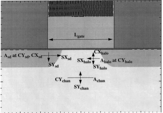
Figure 2.3: An illustration detailing the typical parameters used in analytically describing the complex 2-D doping profiles of a MOSFET. Each impurity has a peak concentration, X and/or Y center positions and associated sigma characteristic roll-off lengths.

Modeling and Design of Experiments. The external parasitic resistance here is determined by varying parameters such as S/D length, thickness, doping and contact material.

Figure 2.5: Design of experiments parameter space surface for RSD as a function of the dominant components of contact resistance and length of the raised S/D.

Figure 2.6: Subthreshold I-V curves for two Leff = 50 nm NMOS devices with different 2-D dop-ing that exhibit the same Ioff, Vt and DIBL at VBS = 0 V. The electrostatics diverge at VBS = -2 V.

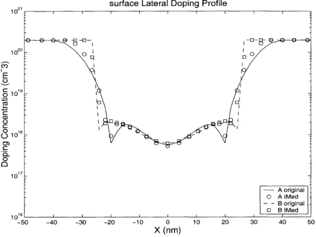
Figure 2.7: Inverse modeling fits using the entire data range showing the lateral doping profiles at the surface for the two Leff = 50 nm NMOS devices with same electrostatics at VBS = 0 V.

Figure 2.8: Order of magnitude error for I-V in parameter space as the example Leff = 50 nm NMOSFET trades off junction depth and lateral roll-off. There is no error for VBS = 0 V but a

global minimum appears for VBS = -2 V.

Figure 2.9: Comparison of the original SUPREM profile to the "re-entrant", "non-re- entrant", and "simple" doping representations: lateral profiles at depth Y = 0 nm show that re-entry is nec-essary to match the Leff.

Figure 2.10: Comparison of the original SUPREM profile to the "re-entrant", "non-re- entrant", and "simple" doping representations: lateral profiles at Y = 20 nm show that the "simple" profile is not complex enough to capture the doping pile-up in the channel (and hence has more error in

its fit to the electrical data).

Figure 2.11: Comparison of the strong inversion I-V characteristics for VDS = 0.2 V, 0.6 V, and 1.2 V on the original SUPREM profile, the "re-entrant", "non-re- entrant", and "simple" doping representations. The more complex doping solutions give less than 5% error.

Figure 2.12: Convergence of an "initial" to "final" parameterized (allowing for 2-D S/D, halo, and two 1-D channel doping features) inverse modeling profile to the original 8e17 cm-3 uniform doping of a 90 nm Leff nFET: in the mid-channel depth profile, the "final" profile matches the original below the depletion depth.

Figure 2.13: Convergence of an "initial" to "final" parameterized (allowing for 2-D S/D, halo, and two 1-D channel doping features) inverse modeling profile to the original 8e17 cm-3 uniform doping of a 90 nm Leff nFET: from the surface lateral profile it is clear that the extraneous halos are suppressed.

Figure 3.1: Cross-section of a t0x = 3.3 nm NMOSFET with Leff - 110 nm depicting I-V

sensitiv-ity via movement of the edge of the depletion region at VGS = 0 V in the substrate with increasing junction reverse bias: depthwise as VBS decreases and laterally as VDS increases.

Figure 3.2: Typical MOSFET 2-D cross-section illustrating Cgds sensitivity to depletion edge in the source/drain. With applied forward VBS (left half) there is more gate controlled depletion than at VBS = 0 V (right half). An accumulation layer will screen the internal fringing capacitance.

Figure 3.3: A flowchart that delineates the ideal comprehensive inverse modeling methodology as a step-by-step procedure from gate stack analysis to determination of a plausible initial guess to a combined log(I)-V & C-V optimization by alternating between data sets to achieve the final 2-D profile.

Figure 3.4: Fit from l-D inverse modeling of long channel subthreshold I-V data for a t0x = 3.3

nm NMOSFET with VBS ranging from 0.5 V down to -3.5 V.

Figure 3.5: An example cross-sectional transmission electron micrograph (TEM) of a L = 30 nm NMOS device fabricated in industry. All non-uniformities such as the configurations of spacer dielectrics and non-planar interfaces must be accounted for in simulations.

Figure 3.6: Inverse modeling fit of the shortest t0x = 3.3 nm device to careful Cgds-V

measure-ments taken at 800 kHz and averaged between four samples per point for varying VBS = 0.5 V, 0

V, and -2 V. The overlap capacitance data for this technology was taken from the stand-alone L = 1 p.m device. The error is within the noise level of 0.025 fF/Mm.

Figure 3.7: Inverse modeling fit of the shortest t0x = 3.3 nm device to subthreshold I-V data for

various biases (VDS = 0.21 V, 0.61 V, 1.21 V) at VBS = 0.5 V, 0 V, and -2 V. The better than 0.08

relative RMS error indicates a converged solution to the 2-D doping profile.

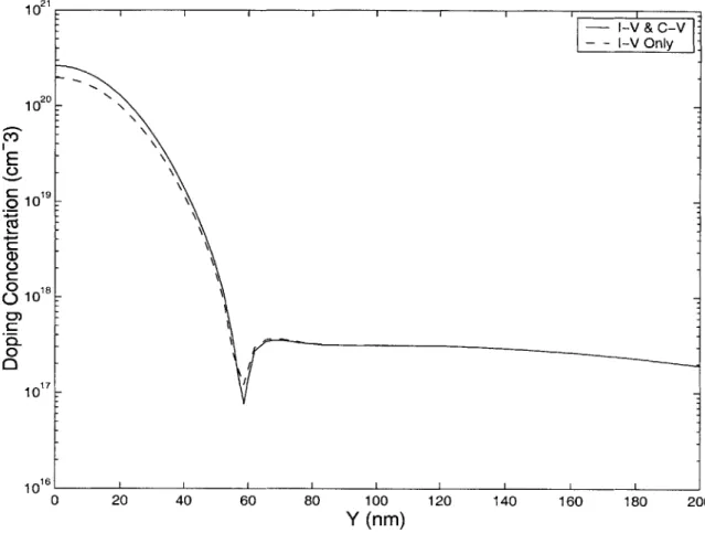
= 3.3 nm device using "I-V & C-V" data versus "I-V Only" data. The methods give roughly the same junction depth but the S/D peak doping in "I-V Only" was arbitrarily set to 1 x102 _cm-3

Figure 3.9: Comparison of the lateral doping profiles at the Si/SiO2 surface for several t0, = 3.3

nm devices with extracted physical Lgate = 100 nm, 130 nm, 160 nm using "I-V & C-V" data ver-sus "I-V Only" data. The log(I)-V data provides sensitivity especially in the channel region while the addition of C-V data determines the S/D peak doping (which has two arbitrary settings of

1x1020 cm-3 and 5x1020 _cm-3 _{for "I-V Only") and slope.}

Figure 3.10: Full Cgg characteristic extracting t0x = 1.5 nm on this L = 10 pm device from an

advanced NMOSFET technology. Due to leakage parasitic resistance, this C-V must be corrected

[15] using two frequencies, here 800 kHz and 400 kHz. The fit exhibits good gate stack modeling

of QM and polysilicon depletion effects.

Figure 3.11: Inverse modeling fit of the shortest t0x = 1.5 nm device to careful Cgds-V

measure-ments taken at 800 kHz and averaged between four samples per point for varying VBS = 0.5 V, 0

V, and -1.5 V. The error is within the noise level of 0.025 fF/Mm.

Figure 3.12: Extracted lateral profiles using the combined inverse modeling technique on t,, =

1.5 nm devices; these short channel MOSFETs have Leff ~ 35 nm, 45 nm, 55 nm, 80 nm, and 120

nm. The longer three lengths all fit to independent Cgds-V measurements. The shorter two lengths had no C-V data but their S/D peak values were fixed at the value obtained for the longer.

Figure 3.13: Extracted depthwise mid-channel doping profiles of the to,, = 1.5 nm technology

devices. The profile approximates the 1-D long channel profile but increases due to merging halos at shorter channels to control short channel effects.

Figure 3.14: Flowchart for optimization of coefficients for processing steps such as diffusion that are simulated with experimental conditions to give a 2-D profile that matches inverse modeling.

Figure 3.15: Lateral doping profiles at the surface from 2-D inverse modeling of t0x = 1.7 nm

NMOSFETs with effective channel lengths of about 30 nm, 45 nm, 60 nm, 95 nm, and 150 nm.

Figure 3.16: Fit of lateral doping profiles of the L = 95 nm device using calibrated "Fermi" point

defect diffusion. While decent, the process simulation has some mismatch in metallurgical junc-tion between the surface and Y = 20 nm deep.

Figure 3.17: Fit of lateral doping profiles of the Leff = 95 nm NMOS device using a calibrated TED diffusion model.

Figure 4.1: Confirmation of the convergence of the simulated drive current of a NMOSFET using EB to the DD model as energy relaxation time goes to zero.

Figure 4.2: Plot of the effective velocity (the Caughey-Thomas mobility times the electric field)

a decreased beta makes it harder for the device to reach velocity saturation.

Figure 4.3: Measured mobility at VDS = 10 mV corrected for field above Vt for long channel devices with high bulk dopings extracted at 1x1017, 8x1017, 1.7x101 8, and 3.9x1018 cm 3

Figure 4.4: Optimization of coulombic mobility dependence as well as universal mobility coeffi-cients using a range of I-V data for the long channel bulk devices with various doping levels.

Figure 4.5: Extracted curve of coulombic mobility versus doping level. The model assumes this mobility (some combination of impurity and phonon scattering) whenever it is under the universal curve. The mobility for minority carriers in bulk tracks this result.

Figure 4.6: technology

Figure 4.7: technology

Measured and calibrated mobility vs. effective field for a nitrided oxide NMOS

with tox = 3.3 nm.

Measured and calibrated mobility vs. effective field for a nitrided oxide PMOS

with tox = 3.3 nm.

Figure 4.8: A simulation of the effective short channel mobility at constant Beff versus Leff

utiliz-ing the calibrated coulombic mobility on the t0x = 1.5 nm NMOS family. The good fit indicates

Figure 4.9: Experimentally observed mobility degradation versus effective channel length in a tox

= 1.5 nm NMOS device family for constant effective field. The triangle symbols represent

simu-lations at various Leff for Eeif of 0.8 MV/cm and 1.1 MV/cm without a Coulomb mobility model.

Figure 4.10: Flowchart outlining the transport model calibration procedure from inverse model-ing, mobility, parasitics, and transport parameters.

Figure 4.11: Calibration of parasitic resistance using strong inversion I-V at low VDS = 10 mV for a tox = 3.3 nm family with a Leff - 110 nm NMOS and Leff 150 nm PMOS device.

Figure 4.12: Fit to strong inversion data for NMOS Leff 110 nm tox = 3.3 nm device with

extracted RSD = 245 Q tm at VGS = 1.8 V.

Figure 4.13: Fit to strong inversion data for PMOS Leff 150 nm tox = 3.3 nm device with

extracted RSD = 600 &4m at VGS = -1.8 V.

Figure 4.14: Measured vs. DD and EB Ion vs. Iof for NMOS tox = 3.3 nm family of Leff 50 nm,

80 nm, 110 nm, 150 nm with VDS = 1.5 V.

Figure 4.15: Comparison of the scaling trends of effective velocities defined as being extracted using the gmi method and the calibrated DD vsat for the NMOS tox = 3.3 nm family.

Figure 4.16: Measured vs. EB Ion vs. Ioff for NMOS tox = 1.5 nm family of Leff - 35 nm, 45 nm, 55 nm, 80 nm, 120 nm with VDS = 1.5 V and 1 V.

Figure 4.17: Measured vs. EB Ion vs. Ioff for NMOS tox = 1.7 nm family of Leff - 30 nm, 45 nm, 65 nm, 95 nm, 150 nm with VDS = 1.5 V and 1 V.

Figure 4.18: Measured vs. DD Ion vs. off for PMOS tox = 3.3 nm family of Leff 70 nm, 90 nm, 150 nm with VDS = -1.5 V; EB calibration coincides (not shown).

Figure 5.1: "Well-tempered" Bulk NMOSFET designed at the Lgate = 13 nm node on the Road Map. The abrupt lateral doping profile at the surface is shown.

Figure 5.2: Design of experiments by varying the halo doping of a Leff = 50 nm NMOSFET with effective tox ~ 2.4 nm. The simulated Ion vs. Iof curve was generated at VDS = VGS = 1.5 V.

Figure 5.3: Template Bulk MOSFET topology showing complicated net doping on the z-axis as a function of the cross-section of the device, here with L = 20 nm.

Figure 5.4: Template MOSFET topology for DG and SG architectures exhibiting raised S/D, spacer, gates, and undoped substrate 2-D cross-section of the device, here with L = 10 nm.

Figure 5.5: The threshold voltage roll-off versus channel length for the template DG device with

Figure 5.6: I-V characteristics at VDS = 1.0 V for the template DG device with mid-gap gates. Gate lengths vary from 38 nm down into the overscaling range to L = 6.5 nm. Multiple

workfunc-tions are extracted by shifting

VGS-Figure 5.7: The density of devices with variation AL = 3 nm around a nominal L = 10 nm is assumed to be a gaussian distribution with 3a = AL. The peak of the power distribution is skewed due to the rapidly increasing Ioff at shorter L.

Figure 5.8: Stand-by power versus gate length of the template DG device at VDD = 1.0 V for var-ious workfunctions from -0.3 V to +0.3 V tracks the exponential rise in off current.

Figure 5.9: Performance versus gate length of the template DG device at VDD = 1.0 V for various workfunctions from -0.3 V to +0.3 V.

Figure 5.10: The trade-off with AL = 2 nm of the template DG MOSFET at VDD = 1.0 V for var-ious $. For each $ curve, the performance (as in Fig. 5.10) and power (as in Fig. 5.9) associated with each L ranging from 38 nm to 6.5 nm is plotted. Fmax is the performance envelope.

Figure 5.11: Ratio of performance to Fmax vs. power of the template DG MOSFET at VDD = 1-0 V for various $ plotted as a function of L, with AL of 1 nm (solid lines) and 3 nm (dashed).

Figure 5.12: The trade-off of performance vs. power of the template DG MOSFET at VDD 0.6 V for various $ plotted as a function of L, with AL = 2 nm.

Figure 5.13: The trade-off of performance vs. power of the template SG MOSFET at VDD 1-0 V for various $ plotted as a function of L, with AL = 2 nm.

Figure 5.14: The trade-off of performance vs. power of the template Bulk MOSFET at VDD 1 -0

V for various $ plotted as a function of L, with AL = 2 nm.

Figure 5.15: The performance envelope trade-off (assuming no AL) versus stand-by power for the template DG, SG, and Bulk devices at operating biases of 1.0 V and 0.6 V.

Figure 5.16: Relative change in stand-by power versus gate length for a 1 nm process variation in Tsi in the template DG at VDD = 1.0 V for various $ from -0.2 V to +0.2 V.

Figure 5.17: Impact on drive current of changing the abruptness cy of the S/D extensions as a

DG device scales with constant DIBL and overdrive, VGS - Vt = 0.7 V, for conditions of having

YES/NO contact resistance.

Figure 5.18: Impact on Ion at constant overdrive and VDS 0.7 V as a DG device scales with con-stant DIBL of having 4x107 Qcm2 (assuming a 10 nm long S/D) or NO contact resistance,

YES/NO to having a 10 nm spacer, or having a 2x1019 cm-3 rather than Ix102 cm-3 S/D.

Figure 5.19: Performance vs. L for the template DG at VDD = 1.0 V bounded by the curves for AL of -2 nm and +2 nm which leads to clock skew.

Figure B.1: Measurement set-up for short channel MOSFETs in order to obtain the log(I)-V and Cgds-V data necessary for inverse modeling.

List of Tables

Table 2.1: For each Road Map node, these initial guess specifications for the MOSFET source/ drain and channel 2-D gaussian doping parameterizations should lead to inverse modeling

Chapter 1

Introduction

1.1 Motivation

As the semiconductor industry continues to shrink transistor sizes into the sub-100 nm regime, accurate characterization of the devices becomes essential. In order to obtain reliable models that will predict the performance of VLSI circuits, physical understanding and tools must be developed to determine both the physical structure of the devices and their transport behavior. This knowledge will then allow for an accurate analysis of the optimal path for sub-50 nm MOS-FET scaling.

Unfortunately, direct characterization methods (e.g., scanning capacitance [1], scanning resistance [2], XTEM [3], or more recently 2-D SIMS [4]) have about one order of magnitude less spatial resolution and minimum doping sensitivity than needed for modem MOSFETs, not to mention that the measurement apparatus and sample preparation can be cumbersome. However, direct characterization may be deemed worth it to obtain an approximation to the doping.

On the other hand, indirect techniques [5] based on inverse modeling [6] using either C-V [7] or weak inversion log(I)-V [8] data have proven effective in extracting the 2-D profiles with required resolution. Whereas Cgds-V (where Cgds = Cgd + Cgs) data can provide good sensitivity for gate to source/drain (S/D) overlap doping features, subthreshold I-V data exhibit strong

dependence on the channel profile, with weak dependence on the transport model and parasitic resistances and capacitances. Additionally, S/D to body diode capacitance has been used as another tool to detect aspects of the doping [9].

29

L7

LII T

4"2

.3B

Figure 1.1: Complex 2-D doping distribution of an Leff = 50 nm MOSFET generated in

SUPREM exhibiting abrupt re-entrant source/drain regions, super-halo channel, and surface dop-ing pile-up.

The complex doping distributions that appear after processing of modemn MOSFETs [10] such as in Fig. 1.1 need all of their important features to be characterized. Hence, the thrust of this thesis will be to research ways to make the indirect, numerical technique of inverse modeling a comprehensive and reliable design evaluation tool for sub-100 nm devices. Furthermore, these results will be used to gain insight into the validity of short-channel transport models and the best path for future MOSFET scaling.

The project will progress through tasks summarized by the following: analysis of the reli-ability of inverse modeling, coding the non-linear optimization loop, performing accurate C-V and I-V measurements on advanced devices, developing an inverse modeling methodology that combines the data sets, inverse modeling of MOSFETs with a spread of channel lengths in multi-ple technology families, developing a methodology to calibrate and evaluate device transport models, study of MOSFET overscaling, designing sub-100 nm bulk and DG MOSFETs, and inte-gration of the inverse modeling results to calibrate process simulation models.

1.2 Organization of the Thesis

The thesis goals and contributions to the field of device engineering are outlined in broad terms in the following paragraphs.

Chapter 2 will commence with a study of the computational techniques needed for the proposed device simulations. Understanding and appropriate choice of device physics models [11] and numerical solution methods, i.e. approximations, are required for accurate results. Then, methods of searching the parameter space, such as the design of experiments, are explored. It is

important to evaluate the reliability of the inverse modeling optimizations to give confidence that the indirectly-obtained profiles are indeed unique.

Chapter 3 develops a technique for combining the log(I)-V weak inversion and C-V data that are most sensitive to the electrostatics of the 2-D gate-stack and doping structure. Fig. 3.1

provides a schematic for performing the idealized inverse modeling methodology. Each stage must have a detailed description of the experimental procedures for measuring the required data. By employing inverse modeling on a variety of sub-100 nm MOSFET technologies, its utility will be realized. The acquired profiles are useful for comparison and modification of process simula-tions.

behavior, it is then possible to investigate carrier transport. It is crucial to select transport models that will have the most physical significance. The methodology [12] used to calibrate these mod-els must isolate the effects of low-field mobility, parasitics, and high-field transport to ensure the extraction of a unique set of transport parameters. The calibrated results can show excellent agreement over a family of device lengths. Also, the short-channel mobility can be explored.

Chapter 5 utilizes accurate models for both MOSFET topology and transport behavior to pursue new paths in scaling [13] to the sub-20 nm regime. For bulk-Si, relationships [14] between device integrity and doping as a function of scaling are developed. A technique of "overscaling" devices beyond the "well-tempered" electrostatic regime yields insight into the performance vs. power trade-off. From these analyses, an optimal double gate design can be infered.

Chapter 2

Computational Techniques for Simulation

2.1 Relevant Device Physics

Before embarking on a project to characterize a device's electrostatic and transport proper-ties, a critical review of the underlying physics relevant to the problem proves useful. The govern-ing equations of electromagnetism [15] and the conservation laws must be solved as well as the statistical and quantum mechanics (QM) [16]. Consequently, analytical models for MOSFET operation are developed. Herein, the coordinate system is defined as Cartesian with X along the length and Y running depthwise of the MOSFET.

The core equations of motion in device simulation mix Maxwell's equations with Boltz-mann transport. Because modem transistor logic is not optical, the Poisson's equation

0 = FV 2 i +q(p-n+Nd-Na)+p = FO Equation 2.1

contains the necessary electrodynamics where E is the material permittivity, V is the potential, q is the elementary charge, p is extra fixed charge, and p, n, Nd, and Na are the hole, electron, donor impurity, and acceptor impurity concentrations, respectively. For most purposes here, macro-scopic approximations underpin the transport computations with the continuity equations

1 an

0 = -V* - n - U

a

o=-Vej - UP -- _q

_at

Equation 2.2

Equation 2.3

where Jn and JP represent the current density for electrons and holes, respectively. The quantities labeled as U indicate the net carrier recombination rates with most processes proportional to (np

-nj2_{), where ni is the intrinsic concentration. In static flow, the time derivates go to zero while}

in = -q On i = -q p pV$,

Equation 2.4 Equation 2.5

represent the densities as a function of mobility, pg, scattering terms and the gradient of quasi-Fermi potentials, $, which include carrier diffusion and drift phenomena due to the applied field.

The interrelation between carrier concentration and potential introduces the role of statisti-cal mechanics. The integral of the density of states multiplied by the population function yields

n = NCF1/₂(nn) p = NVF1/ ₂(1p) - qq - EC ln= _kT kq+ E SP kT Equation 2.6 Equation 2.7

with k as the Boltzmann constant and T as absolute temperature where NC, EC, Nv, and Ev are the effective density of states and energies for the conduction and valence bands edges, respectively, of the solid-state material (such as silicon). Using Fermi-Dirac statistics is necessary for highly doped semiconductors due to the dependence on the difference in quasi-Fermi and band energy in the integral of order 1/2

F _F1/2(Tif) ( = 2 Equation 2.81/2

Jn01 _{+ e"}

d

f

Furthermore, advanced MOSFETs with thin gate dielectrics must account for the QM effect of carrier quantization in the inversion layer. Although solving the Schroedinger equation

[17] for the carrier wave function would be most accurate, for the devices in this study the Van Dort approximation [18] is sufficient and dramatically saves time.

Because the carrier distribution shifts away from the surface, the threshold voltage increases and the energy level splitting of the band gap, Eg, is modeled as

AEg= $ QM T 1/3 E2/3 Equation 2.9

where E1 is the electric field perpendicular to the surface at any grid point, and 3QM is a fitting

factor roughly 4.1 x10-8 _{e V -cm. Also, the QM concentration shifts in the inversion layer by}

-AEg

ni,QM = nie 2kT Equation 2.10

To estimate the effect of further 2-D QM as the gate length decreases to sub-10 nm, con-sider [19] the potential V(x) between S/D as a harmonic oscillator barrier with peak xO

2

qV(x) = 2W (X - x)2 _{kT = ho}

2Tc Equation 2.11

where m is the effective mass and o signifies the curvature. This o can be translated into an effective temperature T. In the L = 6.5 nm simulation of Fig. 2.1, a VDD of 0.6 V induces a

curva-ture in the potential that is less than the curvacurva-ture at T = 300 K, indicating that the S/D tunneling

is still below the thermal off-current. 0.51 0 4-0. 0 -0.5 -1i ) -5 DG Tsi=5nm; Vds=0.6V 0 X (nm)

Figure 2.1: Classical shape of the conduction band in the lateral direction of an undoped L = 6.5 nm MOSFET at VGS = 0 V and VDS = 0.6 V. The band bending lacks enough curvature for the S/ D tunnelling to swamp the thermal current.

Another leakage path across material junctions is band tunneling which is described generically by a Fowler-Nordheim model where a and

@

2 E

J = cE e Equation 2.12

Finally, using a few simplifications of these numerical equations results in an approximate yet handy analytic description of MOSFET operation meant for reference. The C-V

characteris--- Conduction Band

5 10

.. . . .. . . . . . . . ... . . . . . . . -..

tics will be discussed later and their measurement technique is described in Appendix B. In weak inversion, the drive current, ID, is diffusion dominated and exponential with applied voltage yet linear with mobility. In strong inversion, drift is the dominant mechanism. For qualitative refer-ence, the equations [20] for a MOSFET of width W and length L with uniform channel doping, N, in subthreshold condense to

- _{Ixexp VGS- 1 - exp ( Dis]}

L not Ot I2 = _{IX = ot2} X VC ox2 eF )1.50F _{- V S es 29} Equation 2.13 Equation 2.14 Equation 2.15 Equation 2.16 V = V FB + .+ Yef. 5 F - VBS - CDIBL(N, VBs)VDS 2 E qN Yeff = ASCE Co

where

Q,

O, = kT/q, $F is the Fermi potential, VFB is the flat band voltage, Cox is the oxide capacitance,

and yff the body factor along with the drain induced barrier lowering parameter TDIBL and a short-channel-effect fitting parameter ASCE are highly dependent on the doping. For inverted operation, a relatively crude approximation for the current goes linear with voltage until the drain falls below the threshold voltage [21], Vt, at VDS(sat)

L ID ~ fo iDriftdx V _{(sat) = VGS - V} W t _VS-V L ox G VDS - VDs 2] Equation 2.17 Equation 2.18 Vt- VFB + 20F

2.2

Numerical Solutions

If describing the solid-state physics as a set of relevant equations as in the previous section is accurate, then theory shall readily characterize the behavior of any device. However, as in most scientific cases, the complexity of the system demands numerical methods [22] to provide timely self-consistent solutions. These methods, along with techniques to optimize the devices at hand, require an overview to ensure their robustness.

Most sets of nonlinear partial differential equations can be solved accurately by linearizing into matrix form and iterating. When the electrostatics are relatively independent of the conserva-tion laws, decoupled iteraconserva-tions that solve each equaconserva-tion individually are suitable. More generally,

aF(i)Ai = -Fi) Equation 2.19

represents the coupled solution using Newton's method where the Fi are the governing equations (e.g., Eq. 2.1 to 2.3) and A is the update to the unknowns; the matrix in expanded form is

[A~]

_FO]

An

=-FJ

Ap_ F

Equation 2.20

This equation can itself be solved directly using Gaussian elimination, which unfortu-nately becomes computationally intractable for larger problems. Several iterative methods exist to solve the Ax = b matrix problem such as the conjugate gradient method. Fast convergence occurs if A has degenerate eigenvalues when essentially minimizing the residual

r = b-Ax Equation 2.21 aF₀ an aF_1n an aF1, aF₀ ap aFl ap aF1 aFe aFln

aF

For systems involving transient physical behavior, the time evolution is sufficiently

approximated by first or second order difference equations. In the particular case of the small-sig-nal response of a device, the vector x of unknowns is assumed to be of the form

5c = _{x xDC XACe}x- e

j(O*

which leads to a DC solution and a set of AC parameters at frequency w.

C

z

Ci

03-m-Lnue '!1 5 ronw)

Figure 2.2: Plot delineating the 2-D rectangular gridding approach on a archetypal MOSFET with gate stack dielectrics and substrate doping distributions. The mesh becomes finer near regions of heavy transport and where structural details change rapidly.

Of course, the numerical apparatus must solve the aforementioned equations at each grid point in the problem. Thus, the finesse given to meshing issues often determines the ease of

con-vergence. A typical gridding scheme for a MOSFET with a 2-D cross-section of the gate stack and doped substrate is rendered in Fig. 2.2. Although too coarse a mesh fails to capture rapid changes in the potential and carrier distributions, too fine a mesh can lead to unphysical values (e.g., if less than the lattice spacing - 0.5 nm). Moreover, the non-uniform mesh should be as smooth as possible: in the vertical dimension, a good choice grid spacing often varies geometri-cally from 1/3 of gate height at the top to 1/3 of to at the oxide interface (which gives a few mesh lines in the inversion layer) to 1/10 of the substrate thickness at the bottom simulation edge; in the lateral direction, the grid is symmetric about mid-channel and typically ranges from 1/20 of the gate length to half the characteristic length of doping at the metallurgical junction to 1/5 of the spacer at the simulation edge. Since most device features are sufficiently rectangular, the govern-ing equations are solved usgovern-ing finite difference between grid points rather than finite element.

Furthermore, good approximations used as the initial guess to the mesh solution often require projections of previous simulations and small increments to the bias points. A solution is determined to have converged when the error norm (difference between both sides of the equa-tions) is below a specified tolerance. The non-contact materials observe the boundary condition

E awl-

aE2

where the difference in permittivities times the derivatives of the potentials normal to the bound-ary realizes any existing surface charge, us.

The last piece of structural information in standard device simulations is the impurity dis-tribution. A simple yet powerful way to describe the 2-D doping is through a superposition of representation functions where the Aj are the peak doping values

N(x, y) = JAjfXj(x)fYj(y) Equation 2.24

a

Figure 2.3: An illustration detailing the typical parameters used in analytically describing the complex 2-D doping profiles of a MOSFET. Each impurity has a peak concentration, X and/or Y center positions and associated sigma characteristic roll-off lengths.

fXj(x) = exp [(X j)2]

x,f

f Y1(y) = exp[-(y C'2 7

Equation 2.25

Equation 2.26

As depicted in Fig. 2.3, the source/drain (S/D) and halos of the typical MOSFET are rep-resented analytically by 2-D gaussians with center positions C, and CY, and characteristic lengths aT and (Y ; the channel implants usually take the form of 1-D gaussians.

Finally, with a reasonable device simulator in place, optimization of device parameters [23] becomes feasible. A non-linear optimizer such as Levenburg-Marquardt algorithm [24] takes

F(P) = 2 = [ (sim) _ (expt) 2 Equation 2.27

the sum, F, of squared errors hi between simulated and experimental electrical data yj and tries to minimize it with respect to the vector of parameters, P, to be optimized with

VpF = 2J T = 0 Equation 2.28

where J signifies a special matrix containing the sensitivity of each data on each parameter

J- = Equation 2.29

called the Jacobian. To find the zeros of the gradient of F, once again apply Newton's method

[2J

to reduce the problem to solving Ax = b for the parameter updates Aji using the matrix

2

HU =Equation F 2.31

apiapj

called the Hessian. The magnitude of the elements of the matrix H also indicate the sensitivity to a particular pair of parameters. For practicality, the algorithm approximates the Hessian as

H~2J J+XD Equation 2.32

where D is a matrix with only the diagonal of J. The optimization begins as a steepest descent method with large 1 which is then reduced every iteration. Until the desired data error tolerance is met, the parameters of the ith iteration are revised as

i+ = + Equation 2.33

To conclude, an analysis of the time per iteration based on a computer's intrinsic speed rsim which is multiplied by the size of the mesh, data, and number of parameters is

Titeration = (1 + npara) * ndata - node * Tsim Equation 2.34

2.3 Searching the Parameter Space

When designing or evaluating a device, it would be handy if one could accurately predict how changing certain device parameters [25] would affect certain characteristics and measures of performance. Inverse modeling is a technique which accomplishs these tasks through a numerical optimization procedure. Another mathematical method is the Design of Experiments which searches many parameters in as few as possible combinations, runs experiments to obtain the desired characteristics, and generates a multi-dimensional response surface fitted to these values.

A choice of parameters with both efficiency and accuracy for the Design of Experiments is the Central Composite Design (CCD). Each of N parameters is assigned a range of values includ-ing a minimum, midpoint, maximum. There are also two "2-Level" points equidistant from the

conducted: 1) runs of all combinations of parameters being at 2-Level points; 2) a centerpoint (all

parameters at the midpoint) run counted about 3 x times; and 3) axial runs of the minimum and maximum of a particular parameter with the midpoints of the others. A general purpose C++ program has been written to carry out this procedure. A standard device simulator performs the runs and the desired figure of merit output is then tabulated. Last, a statistical mathematics pack-age such as SPLUS is utilized to compute a non-linear least squares fit of the data to a response manifold.

Inverse Modeling I Design of Experiments: Parasitics

Z--n+ polysilicon

spacpr

inversion, R R R

extension oping +Pcontac

deep

S/D

Figure 2.4: Example structure of the drain region of a MOSFET under investigation using Inverse Modeling and Design of Experiments. The external parasitic resistance here is determined by varying parameters such as S/D length, thickness, doping and contact material.

The simulated test structure of Fig. 2.4 depicts the drain region of a MOSFET that can be investigated by different methods. For example, the Design technique has been used to study the

changes in the parasitic S/D resistance, RSD, in a raised contact SOI NMOSFET. A small 0.1 V potential was applied from an artificial "contact" at the inversion layer to the raised contact; thus, RSD can be calculated as twice the voltage divided by the drain current. The arbitrarily chosen features include a raised S/D height of 60 nm with a silicide contact extending down 40 nm from the top, and a donor concentration of 2x1020 cm-3in the deep S/D region.

1000 800 -J. E E .C 6001 400.1 200-,. 5 x 10-7 4 0.3 3 - -0.25 . . . -0.2 2 _0.15 R.CONT (Ohm*cm2) 1 0.1 L.RAISE (um)

Figure 2.5: Design of experiments parameter space surface for RSD as a function of the dominant components of contact resistance and length of the raised S/D.

Several experiments were then conducted varying the following parameters: length of the S/D, L.EXT, from 13 to 37 nm; length of the raised region, L.RAISE, from 100 to 300 nm; SOI thickness, YSOI, from 10 to 30 nm; doping concentration in the S/D extension, D.EXT, from

Picking the midpoints for L.EXT, Y.SOI and D.EXT, one can render the response surface for RSD in Fig. 2.5 as a function of the two dominant parameters R.CONT and L.RAISE. Most of the resistance components follow the physically intuitive dependence

= pLength

Area Equation 2.35

where p is resistivity and the proportionality is linear with length and inverse with contact area.

log(I)-V Data; Vbs = OV, -2V 10 106 10-7 102 10-1014 1015 A: Vds = 0.21V, 0.71V, 1.21V - - B: Vds = 0.21V, 0.71V, 1.21V --0.2 -0.1 0 0.1 0.2 Vgs (V) 0.3 0.4 0.5

Figure 2.6: Subthreshold I-V curves for two Leff = 50 nm NMOS devices with different 2-D

dop-ing that exhibit the same Ioff, Vt and DIBL at VBS = 0 V. The electrostatics diverge at VBS = -2 V.

The trickiest step of this method is coming up with an appropriate fitting function that minimizes the error. In general, this formula consists of linear, inverse linear, higher order, and

cross terms. In practice, it requires knowledge of the underlying physics as

RSD = _{+ k OLEXT + L + ki1LRAISE}

LRAISE

ki ki2 RCN

+ _SoI + k12YSOI + _EXT + k1 3DEXT+ kl4RcoNT + k24RCONT2 + kCLONT_RAISE

Equation 2.36

where the k's are fitted coefficients. From Eq. 2.X, one justifies the linear dependence on L.EXT and the mostly inverse linear depedence on YSOI, D.EXT (resistivity varies inversely with dop-ing), and L.RAISE (proportional to contact area).

1021 10 20 E S19 o010 C.) o 18 U) 10 0) 0 10 17 1 016 -5

surface Lateral Doping Profile

-o a0-80 e - --- A original 0 A iMed - - B original o B iMed -40 -30 -20 -10 0 10 20 30 40 50 X (nm)

Figure 2.7: Inverse modeling fits using the entire data range showing the lateral doping profiles at

the surface for the two Leff = 50 nm NMOS devices with same electrostatics at VBS = 0 V.

Even with good means of searching parameter space, one must verify how broad a range

of electrical data is necessary to ensure a unique profile. As an exercise, two simulated Leff = 50

nm NMOS devices have been constructed with identical electrostatic qualities (i.e., I, Vt and DIBL) at a back bias, VBS = 0 V, as in Fig. 2.6. Device A trades off the electrostatic influence of a gradual S/D with a short junction depth, xj, of 25 nm while B has an abrupt fall-off and an xj of 40 nm; the halos are modified slightly to maintain the desired I-V.

-- Vbs = OV -e- Vbs = -2V 1 0.8 -20.6 -00.4 0 0.2-0 -45 40-35 _{- 8} 30 6 25 2 4 xj (nm) 20 0 _{sigma,x (nm)}

Figure 2.8: Order of magnitude error for I-V in parameter space as the example Leff = 50 nm NMOSFET trades off junction depth and lateral roll-off. There is no error for VBS = 0 V but a global minimum appears for VBS = -2 V.

However, as soon as a broad range of bias is included in the log(I)-V data, the difference in electrical signature becomes apparent. In fact, it is only through utilizing this difference in electri-cal data that the optimization loop was able to distinguish between the two dissimilar doping pro-files as in Fig. 2.7. The lateral cut of the 2-D profile shows that a wide range of data, in this case

VBS = -2 V which detects doping deeper, is vital to ensure that the inverse modeling method cap-tures all existing topological device feacap-tures. If there are no electrical data sensitive to a particular feature, detection cannot be expected.

To further highlight the importance of selecting a broad range of data, the error is plotted as a function of the parameter space variables xj and a, in Fig. 2.8. The line of zero error

repre-sents a continuum of devices that trade-off between depthwise and lateral junction parameters. Going along the same multi-variable path but looking at the error for VBS = -2 V produces an error curve relative to the I-V data for the device with the midpoint doping parameterization. Clearly, using more data is a means of obtaining a true global minimum. The graphical depiction of error accentuates how the optimizer calculates the updated search direction and verifies that enough sensitivity exists to extract the parameters.

2.4 Reliability of Optimizations

While the potential power of inverse modeling in 2-D profiling of sub-100 nm devices is evident, it would be ideal to have a means of characterizing the reliability of this technique. How-ever, since no direct approach can currently verify the modeling results, we resort to a heuristic

assessment. The most obvious question is how close the simulated electrical data from the inverse modeled device agree with the experimental electrical data. From a wide array of inverse model-ing experience, it is found that the majority of converged results typically exhibit relative RMS errors below 0.1.

All positions reference mid-channel as X = 0 and the surface as Y = 0. The starting value for the S/D extension peak doping, Asd, is 2x1020 cm-3 which extends down uniformly to a center Y position, Cysd, of 5 nm beyond which it starts to roll-off. As for the halo centers, Cx,h is

xj, which is tracked by

Cy'c-Ah AC

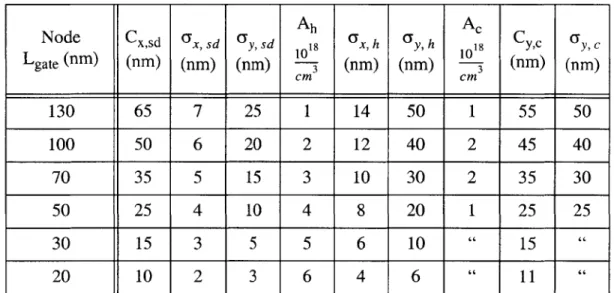
Node Cx,sd , sd ysd 10 18 ax, h y, h 1018 yC y, C

Lgate (nm) (nm) (nm) (nm) -i (nm) (nm) cm (nm) (nm) 130 65 7 25 1 14 50 1 55 50 100 50 6 20 2 12 40 2 45 40 70 35 5 15 3 10 30 2 35 30 50 25 4 10 4 8 20 1 25 25 30 15 3 5 5 6 10 15 20 10 2 3 6 4 6 11

Table 2.1: For each Road Map node, these initial guess specifications for the MOSFET source/

drain and channel 2-D gaussian doping parameterizations should lead to inverse modeling conver-gence given a broad enough range of electrical data.

How easy is it to achieve convergence to the global minimum error with a given parame-terization? Taking the aforementioned sum of two 2-D gaussians for the S/D and halos and 1-D gaussian for the channel as the doping representation functions, Table 2.1 quantifies inital guess parameter values for each Lgate node that should lead to convergence. The estimates for charac-teristic roll-off lengths derive from experience in modeling industry devices: the S/D is typically twice as abrupt as the halos. Also, the super-steep retrograde channel doping is not very signifi-cant for the shortest nodes which are essentially super-halo devices. If numbers for an intermedi-ate node are desired, simple interpolation of the doping level trends will suffice.

More challenging questions present themselves regarding the ideality of the final set of doping function parameters. Does the converged parameter set actually represent the original pro-file? An equivalent statement is whether the solution becomes unique using the given doping rep-resentation functions. Furthermore, how closely does the inverse modeled parameterization approximate the real 2-D doping distribution? Perhaps even more significant, how complex should the parameterization be to obtain the best fit and to what extent can this choice of

represen-tation functions be applied generally? A promising strategy to attack these questions is via quali-tative numerical studies because direct methods are too inaccurate.

Original - - Re-entrant -- Non-Re-entrant .... Simple -80 -60 -40 -20 0 X (nm) 20 40 60 80 100

Figure 2.9: Comparison of the original SUPREM profile to the "re-entrant", "non-re- entrant", and "simple" doping representations: lateral profiles at depth Y = 0 nm show that re-entry is nec-essary to match the Leff.

To evaluate the uniqueness of inverse modeling solutions, a virtual nFET that exhibits the super-halo characteristic [26] with 50 nm Leff and 2 nm physical t0x was generated in

TSUPREM4 using Monte Carlo implantation and a RTA with a transient enhanced diffusion model. The doping profiles for this virtual symmetrical device are quite complex, exhibiting re-entrant and box-like S/D features with halos spiking prominently at the surface and washing together deeper in the channel, being quite far from simple gaussians. In this approach, knowing the original 2-D doping allows for a qualification of the inverse modeling. Three inverse

model-E c 19 O010 -C 0) C 0 C 10 17 10 -1C 0

ing representations of the virtual device of decreasing complexity were used: "re-entrant" (a 2-D gaussian for each S/D and halo with peak at depth Y >0, plus a 1-D gaussian background), "non-re-entrant" (same but with peak at Y = 0), and "simple" (uses the non-re-entrant 2-D gaussians only). Fig. 2.9 and Fig. 2.10 compare the original with the extracted profiles at two depths. The corresponding converged log(I)-V RMS error is 0.01, 0.02, and 0.12; futhermore, the C-V RMS error is 0.003, 0.010, and 0.019 fF/pm, respectively.

- - - - - - -- Original - Ii - - Re-entrant -- Non-Re-entrant -.... Simple -80 -60 -40 -20 0 X (nm) 20 40 60 80 100

Figure 2.10: Comparison of the original SUPREM profile to the "re-entrant", "non-re- entrant", and "simple" doping representations: lateral profiles at Y = 20 nm show that the "simple" profile is not complex enough to capture the doping pile-up in the channel (and hence has more error in its fit to the electrical data).

For each parameterization, the solution converges as close as possible to the real doping. Evidently, the better the parameterization, the better the fit to data (i.e., the smaller the RMS error), and the better the fit to doping. This main conclusion regarding the uniqueness and ideality

10 21 1020 E c 19 O010 U 0 C)10 0~ 10 17 10161 -10 0

of possible parameterizations can be phrased independently of which electrical data sets are used in the optimization loop. The "re-entrant" profile is needed to match the longer channel length at the surface, and agrees to better than a factor of two with the original profile except at the peak doping where the re-entry has diminished the peak level. While the log(I)-V data has tried to cause the representation functions to match the Leff at all depths, the inverse modeling has made a compromise by maintaining a S/D peak doping that fits the C-V data as close as possible. While even the "non-re-entrant" doping fits the original after a certain depth, the "simple" representation cannot account for the background created by the merging of the halos in the channel.

SUPREM 50nm NMOS; Vbs = OV; Vds = 0.2V, 0.6V, 1.2V 1 0.9 - 0.8- 0.7- 0.6- 0.5-E 0.4- 0.3- 0.2-- Original 0.1 --- Re-entrant -e Non-Re-entrant -o Simple 0 0.2 0.4 0.6 0.8 1 1.2 Vgs (V)

Figure 2.11: Comparison of the strong inversion I-V characteristics for VDS = 0.2 V, 0.6 V, and 1.2 V on the original SUPREM profile, the "re-entrant", "non-re- entrant", and "simple" doping representations. The more complex doping solutions give less than 5% error.

into possible errors in the strong inversion data are important if one were to use inverse modeled profiles in transport studies. In Fig. 2.11, the more complex dopings exhibit less than 5% error in the output I-V characteristics while the "simple" profile has about 12% error at several voltages. The important conclusion from this exercise is that the electrical and doping fits improve as the representation functions are given increasing degrees of freedom to approximate the profile. A modified parameterization with lateral S/D extension fall-off as a function of Y and variable peak to capture the Leff and the S/D doping level at all depths would be required. The most general representation function is theoretically a sufficiently fine grid 2-D spline function, but simulation time for the optimization would be prohibitive.

MOSFET; mid-channel Depth Doping Profile

10 19 E C 0 0 0 CL 0 O010 16 20 40 60 80 100 Y (nm) 120 140 160 180 200

Figure 2.12: Convergence of an "initial" to "final" parameterized (allowing for 2-D S/D, halo, and two 1-D channel doping features) inverse modeling profile to the original 8e17 cm-3 uniform doping of a 90 nm Leff nFET: in the mid-channel depth profile, the "final" profile matches the original below the depletion depth.

Original

--...- _{Initia l}

- - Final

10 15 0

One must emphasize that it is not intuitive that simply adding more doping parameters and making the representation more and more general will always lead to a more realistic profile. Will a very detailed parameterization (e.g., "re-entrant") work in the general case of trying to inverse model an unknown profile? Towards answering this question a device with minimal dop-ing features such as uniform channel dopdop-ing was inverse modeled startdop-ing from a complicated "initial" guess (2-D gaussian S/D and halos, plus two 1-D gaussian channel profiles); the results are displayed in Fig. 2.12 and Fig. 2.13. As anticipated for a robust algorithm, the "final" profile converges to the uniform doping within the limit of depletion depth, which defines the region of log(I)-V sensitivity; any extraneous functions (e.g., halos) are suppressed as shown in the lateral profile.

MOSFET; surface Lateral Doping Profile

10 21 0 2 0 19 8 017 10 16 -1 I I I I I I - I I I

r

Figure 2.13: Convergence of an "initial" to "final" parameterized (allowing for 2-D S/D, halo, and two 1-D channel doping features) inverse modeling profile to the original 8e17 cm-3 uniform doping of a 90 nm Leff nFET: from the surface lateral profile it is clear that the extraneous halos are suppressed. E C) C., 0 0

In conclusion, the simulations performed in this thesis draws on rigorous computational techniques that describe the device physics and allow for optimization. A broad range of data exhibiting electrical signatures to the actual 2-D features will reliably extract the MOSFET topol-ogy given a parameterization with the corresponding doping representation functions.

Chapter 3

Combined I-V and C-V Inverse Modeling

3.1 Comprehensive Methodology

As MOSFETs scale into the sub-100 nm regime, knowledge of the two-dimensional (2-D) doping distribution is critical for accurate device analysis, process calibration, and compact circuit modeling. This work demonstrates and evaluates a comprehensive inverse modeling technique

[27] that combines the sensitivities of log(I)-V and C-V data. As discussed, the highlights of employing log(I)-V data are high dependence on both lateral (through VDS variation to bring out short channel effects) and depthwise (through varying VBS and depletion depth) doping features including the S/D to bulk junction with associated doping gradients as well as the non-uniform 2-D channel doping distributions. The 2-2-D cross-section in Fig. 3.1 plots the edge of the channel depletion region in the off-state as a function of multiple VBS and VDS; the 2-D sensitivity is quite apparent.

The main advantage of adding the C-V data [28] to the optimization is their sensitivity to the physical gate length and to the shape of the S/D overlap region, including detection of the peak doping (through depletion of part of the highly doped extension). With this more coherent and complete methodology, the indirect characterization of 2-D MOSFET topography may prove itself a dominant device engineering tool in the deep sub-100 nm regime.