1
Debunking the Stereotype of the Lazy Welfare Recipient:
Evidence from Cash Transfer Programs Worldwide
1 Abhijit Banerjee, MITRema Hanna, Harvard Gabriel Kreindler, MIT Benjamin A. Olken, MIT
ABSTRACT
Targeted transfer programs for poor citizens have become increasingly common in the developing world. Yet, a common concern among policy makers – both in developing as well as developed countries – is that such programs tend to discourage work. We re-analyze the data from 7 randomized controlled trials of government-run cash transfer programs in six developing countries throughout the world, and find no systematic evidence that cash transfer programs discourage work.
I. INTRODUCTION
Governments in the developing world are increasingly providing social assistance programs for their disadvantaged citizens. For example, in a recent review of programs worldwide, Gentilini et al (2014) find that 119 developing countries have implemented at least one type of unconditional cash assistance program and 52 countries have conditional cash transfer programs for poor households. Thus, on net, they find that 1 billion people in developing countries participate in at least one social safety net.2
1 Contact email: bolken@mit.edu or rema_hanna@hks.harvard.edu. We thank Alyssa Lawther for excellent research assistance. This study would not have been possible without the many researchers who provided their data to us (or to the public-at-large) and we thank them wholeheartedly for their efforts. All of the views expressed in the paper are those of the authors, and do not necessarily reflect the views any of the many institutions or individuals acknowledged here.
2 These programs serve to transfer funds to low-income individuals and have been shown to have led to reductions in poverty (Fiszbein and Schady 2009) and to have positive effects on education (Schultz 2004, Glewwe and Olinto 2004, Maluccio and Flores 2005) and health services (Gertler 2000, Gertler 2004, Attanasio et al. 2005). However, despite this, policy-makers are often concerned about whether transfer programs of this type discourage work. And indeed, in developed country policy contexts, some transfer programs have indeed been shown to have small, but statistically significant, effects on work.3 On the other hand, despite occasional claims in policy circles to the contrary, there is little rigorous evidence showing that transfer countries in poor countries actually lead to less work, with most existing evidence finding little or no effect of transfer programs on labor supply (see, for example, Alzua, Cruces, and Ripani, 2013; Parker and Skoufias, 2000).
In this paper, we re-analyze the results of seven randomized controlled trials of government run cash transfer programs from six countries worldwide to examine the program impacts on labor supply.4 Re-analyzing the data allows us to make comparisons that are as comparable as possible, using harmonized data definitions and empirical strategies. Re-analyzing the micro data directly also allows us to pool effects across studies to yield tighter bounds than would be possible from any single study.
In this paper we bring together data on this issue from the randomized control trials (RCT) that we could find that met three criteria:5 it was an evaluation of a (conditional or unconditional) cash transfer program in a low-income country that compared the program to a
3 See for example, Ashenfelter and Plant (1990) analysis of the Seattle –Denver Maintenance Experiment or Imbens, Rubin, Sacerdote (2001) estimates of the effect of unearned income on work from studying lottery winners.
4 This extends Alzua, Cruces, and Ripani (2013), which explores the program impacts on labor outcomes for three of the programs that we include. While we use slightly different specifications to harmonize across the full set of datasets that we include, our findings echo theirs.
5 This is a work in progress and we are still continuing to accumulate datasets from additional RCTs that fit these criteria.
3 pure control group; we could obtain micro data for both adult males and females from the evaluation; and the randomization needed to have at least 40 clusters (more details on these restrictions can be found below). To date, this yielded data for programs from six countries: Honduras, Indonesia, Morocco, Mexico (2 different programs), Nicaragua, and the Philippines.
Across the seven programs, we find no observable impacts of the cash transfer programs on either the propensity to work or the overall number of hours worked, for either men or women. Pooling across the five comparably designed studies to maximize our statistical power to detect effects if they exist, we again find no observable impacts on either work outcome.
Theoretically, the transfers could have different effects on work outside the household versus self-employment or work within the family. For example, one could imagine that the effect for outside work sector may be larger, as individuals fear—rationally or otherwise—that formal work employment could disqualify them from receiving future transfers. Looking at the pooled sample, we find a small, significant negative effect on work inside the household (about 1 percentage point, significant at 10 percent level). However, we find no observable effect of the transfers on work outside the household (if anything, while statistically insignificant, the estimated treatment effect is positive).
In short, despite much of the rhetoric that cash transfer programs lead to a massive exodus from the labor market, we do not find overwhelming evidence to support these claims.
II. DATA, EMPIRICAL STRATEGY AND SAMPLE STATISTICS
In this section, we first describe the data and then detail our empirical strategy. In the last sub-section, we provide sample statistics to provide a descriptive picture of each program area.
4 A. DATA AND PROGRAM DESCRIPTION
We began by identifying randomized evaluations of cash transfer programs in low-income nations. For a study to be included, it needed to have both a pure control group and at least one
treatment arm of a conditional or unconditional cash transfer program. In several of the studies that we identified, the authors had randomized across different variants of a cash transfer program or compared cash to in-kind transfers, but did not have a pure control group. These studies provide us with valuable information about how outcomes change based on the program design features, but do not provide us with the overall effect of having the program to begin with and thus are excluded from our analysis.
In total, to date, we identified 18 RCTs that met the above criteria.6 Of these, three were excluded because they did not include variables on both male and female adult labor supply in the public datasets,7 two were excluded due to having fewer than 40 clusters,8 and to date we have been unable to obtain data for another six studies.9
Therefore just 7 RCTs were included in this analysis: Honduras’ PRAF II, Morocco’s Tayssir, Mexico’s Progresa and PAL, Philippines’ PPPP, Indonesia’s PKH, and Nicaragua’s RPS. A notable characteristic of all 7 programs is that they are implemented by national governments (as opposed to NGOs) either as pilot or expansion programs, and thus are
6 We apologize in advance if we have missed a particular study that meets our criterion. Please contact us if you believe we have omitted a potential RCT from this list.
7 Ecuador’s BDH (Edmonds and Schady, 2012; Schady and Caridad Araujo, 2008), Columbia’s SCAE (Barrera-Osorio et al, 2011), and Nicaragua’s Atención a Crisis (Macours et al, 2012).
8 Treatment status was randomized over 8 communities in Malawi’s SCT program (Covarrubias et al, 2012) and over 28 locations in Kenya’s CT-OVC. Despite having a larger number of households in both experiments, the small number of randomization units biases one towards not being able to measure a statistically significant effect unless the effect size is very large; therefore, we did not include them.
9 These include Kenya’s Give Directly (Haushofer and Shapiro, 2013), Tanzania’s TASAF (Evans, Hausladen, Kosec, and Reese, 2014), Burkina Faso’s NCTPP (Akresh, De Walque and Kazianga, 2013), Uganda’s cash transfer to pre-schools (Gilligan and Roy, 2013), Zambia’s Child Program (American Institute for Research 2013) and the Malawi - Schooling, Income, and Health Risk Impact Evaluation Household Survey (Baird, McIntosh, and Ozler, 2011). Some of these datasets are not publicly available and thus cannot be included in our analysis. Others we are in the process are acquiring and we hope to include in future paper drafts.
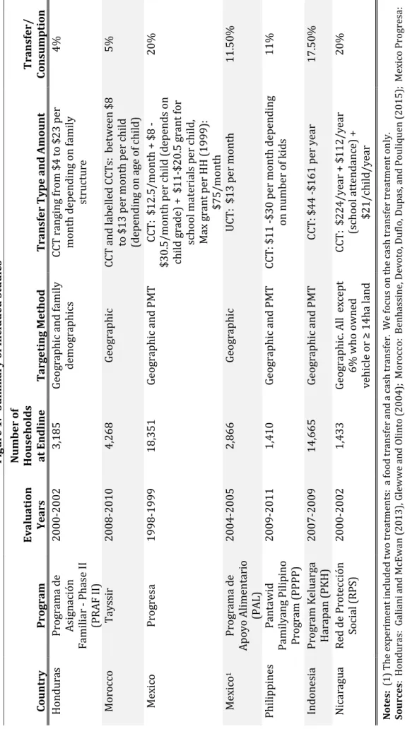
5 Figu re 1 : Sum mar y o f I n cl ude d S tud ies Co un tr y P ro gra m Eval uat ion Y ear s N umber o f H ouseho lds at End li n e Tar ge ti n g Me thod Tra n sfer Ty pe an d Amo un t Tra n sfer / Co n su mpt io n Hon dura s Pr og ram a d e A si gn ac ión Fam ili ar - Pha se II (P RA F II) 2000 -2002 3, 185 Geog raph ic an d fam ily dem og raphi cs CC T r ang in g from $ 4 t o $23 p er m ont h d epen di ng on fa m ily stru cture 4% Moro cc o T ays si r 2008 -2010 4,2 68 Geog raph ic CC T an d labelled CC T s: b etween $8 to $1 3 p er m ont h per chi ld (depen di ng on ag e of ch ild) 5% Mex ic o Pr og res a 1998 -1999 18,351 Geog raph ic an d PM T CC T : $12. 5/m ont h + $ 8 - $30. 5/m ont h per chi ld ( depen ds on ch ild g rade) + $11 -$ 20 .5 gran t for sc ho ol m ate ri al s p er ch ild , Max g ran t per HH ( 1999): $75/ m ont h 20 % Mex ic o 1 Pr og ram a d e A poy o A lim ent ari o (P A L) 2004 -2005 2, 86 6 Geog raph ic U CT : $13 p er m ont h 11.50 % Phi lipp in es Pan tawid Pam ily ang P ili pi no Pr og ram (P PP P) 2009 -2011 1,410 Geog raph ic an d PM T CC T : $11 -$ 30 p er m ont h depen di ng on num ber o f k id s 11% Indon es ia Pr og ram K elu arg a Harapan (P KH) 2007 -2009 14 ,665 Geog raph ic and PM T CC T : $44 -$ 161 per year 17.50 % N ic arag ua Red de P rote cc ión Soc ial (R PS ) 2000 -2002 1, 433 Geog raph ic . A ll ex cept 6% w ho ow ned veh ic le or ≥ 14ha lan d CC T : $224/y ear + $112/y ear (s cho ol att end anc e) + $21/ ch ild/y ear 20% N ot es: ( 1) The e xpe rim en t i nc lude d tw o tr ea tm en ts : a food tr an sf er a nd a ca sh t ra ns fe r. W e focu s on th e ca sh t ra ns fe r tr ea tm en t o n ly. Sources : Ho ndura s: G al ia ni an d M cE wa n (2013) , G le w w e an d Ol in to (20 04) ; M or oc co: B en ha ss in e, D evot o, Dufl o, Dupa s, an d Po ul iq ue n (2 015 ); M exico Pr og re sa : Pa rk er a nd Sk oufia s (2000) ; Sk oufia s an d di M ar o (2008 ); Me xico PAL : Sk oufia s, U na r, an d G on za le z-Coss io (201 3) ; P hil ipi nn es : Cha udh ury , F rie dma n an d O nish i (2013) ; In don es ia : W or ld B an k Of fic e Ja ka rta ( 20 11) ; N ic ar agua : M al uc cio an d Fl or es ( 2005)
6 representative of “real-world” cash transfers. Figure 1 provides some summary details about the programs and evaluation data and provides references to key academic papers for each program.
In terms of program type, most of the programs that we include are conditional cash transfer (CCTs), where benefits are “conditional” on desirable social behaviors, such as ensuring your children attend school and get vaccinated. The two exceptions to pure CCT programs were: (1) Mexico’s PAL program, where benefits were not conditioned on behaviors10 and (2) Morocco’s Tayssir program, which had two treatment arms consisting of a CCT and a “labeled” cash transfer in which the conditions were recommended but were explicitly not enforced. In general, it is important to note that there is considerable variation in how stringent conditions are enforced across countries, so even in programs that profess conditionality, beneficiaries may still receive the full stipend amount regardless of whether they meet them.
A first challenge in these types of programs is finding the poor (“targeting”). Unlike developed countries, where program eligibility can be verified from tax returns or employment records, developing country labor markets often lack formal records on income and employment and thus alternative targeting methods must be used (see Alatas, et al, 2012, for a description). For all of the programs in our study, regions were first geographically targeted based on some form of aggregate poverty data. After that, in 5 out of the 7 programs eligibility was determined by a demographic criterion (e.g. a woman in the household was pregnant or there were children below an age cutoff) and/or an asset-based means test (e.g. not owning land over a certain size).
Once a household becomes eligible for any of the programs that we study, the amount of benefit that one receives is the same regardless of actual income level and lasts at least a period between 2 and 9 years, depending on the program. This differs from many U.S. transfer
7 programs (e.g. EITC, SNAP), where the stipend depends (either positively or negatively) on family income, and is updated frequently. This discrepancy likely stems from the greater difficulty in ascertaining precise income levels in data-poor environments. However, similar to the U.S programs, the level of the transfer received was determined, at least in part, by the number of children in the family and their ages. On net, however, the programs were fairly generous ranging from 4 percent of household consumption (Honduras’ PRAF II) to about 20 percent (Mexico’s Progresa).
For each evaluation, we obtained the raw evaluation micro-datasets from either online downloads or personal correspondence with the authors. Note two features of the evaluation design that affects the analysis. First, all of the studies that we consider are clustered-randomized designs, i.e. the program was clustered-randomized over locations rather than individuals. Thus, in the analysis below, we cluster our standard errors by the randomization unit. Second, we have both baseline and endline data for 5 of the studies. Baseline data were not collected for the Philippines’ PPPP. Moreover, the baseline data for the treatment group of the Honduras’ PRAF II study was collected in a different agricultural season than for the control group (Glewwe and Olinto 2004). Alzua, Cruces, and Ripani (2013) point out that this leads a small but statistically significant imbalance in labor supply between the two groups and, therefore, we decided not to use the baseline for this program. Thus, as we discuss below, we use a different empirical strategy for the programs with baseline data and those without.
While some of the studies had explored impacts on some of the work variables, the sample composition and work variable definitions varied across the studies. Thus, we harmonized the datasets. First, we attempted to restrict our datasets to include all adult males and females, aged 16 to 65, from eligible households. We have two exceptions to this, where we included adults in all surveyed households (regardless of eligibility status): First, Nicaragua’s
8 RPS contains a random sample of households. About 6 percent of households were excluded from the cash transfer program based on a proxy means test, but we cannot identify them in the data. Second, Honduras’ PRAF II has a random sample from households in the geographically targeted areas; we attempted to code the eligibility rules within the evaluation dataset, but did not yet feel fully confident in our ability to back out eligible households.
Next, for these samples, we coded consistent variables for employment status and hours worked per week for each included individual.11 Note two important features of our data set-up: First, our sample includes all individuals, regardless of whether or not they are in the labor force. Thus, if cash transfers induce individuals to exit the labor force, this will be captured by our employment variable. Similarly, individuals who are do not work are counted as “zero” hours of work in our analysis; thus, this variable is capturing both the decision to work (extensive margin) and the number of hours worked (intensive margin). Second, we lack information on hours of work for Indonesia’s PKH program, so it is only included in the analysis on employment status.
In the poor areas where the programs that we analyze are located, a significant share of people work in agriculture (in rural areas) or in self-employment. We include both these activities in the employment status, and we later analyze two outcome variables that differentiate between household work (any self-employed activity) and work outside the household (casual or permanent employment).
11All programs except Morocco ask about the number of hours worked during the last week. In Morocco the
9 B. EMPIRICAL STRATEGY
We begin our analysis by first estimating the effect of being randomized to receive a transfer program on labor market outcomes. Due to the randomization of who received the program, the treatment and control groups should be similar on average, except for receiving the program. Thus, one can estimate the following regression:
Eq 1: 𝑦𝑖𝑐 = 𝛽𝑇𝑟𝑒𝑎𝑡𝑐+ 𝜇𝑠(𝑐)+ 𝜸 ⋅ 𝑿𝑖𝑐+ 𝜀𝑖𝑐
where 𝑖 is an individual in cluster (randomization unit) 𝑐. 𝑦𝑖𝑐 is individual i’s labor market outcome, either an indicator variable that takes the value of 1 if the individual is employed or a continuous variable on the hours an individual worked per week. 𝑇𝑟𝑒𝑎𝑡𝑐 is an individual variable that equals 1 if individual was randomly assigned to the treatment group and zero otherwise; 𝛽 is the parameter of interest, providing the difference in work outcomes between the treatment and the control group.
Note two features of the specification. First, while the randomization should ensure that 𝛽 capture the causal impact of the program, we can include additional control variables to improve our statistical precision. Specifically, we include strata fixed effects (𝜇𝑠(𝑐)) and a number of individual-level control variables (𝜸 ⋅ 𝑿𝑖𝑐), including age, age squared, household size, years of education, and a dummy variable for being married or in a partnership. For each control variable, we code missing values at the variable mean and include a dummy variable that indicates the observations with missing values. Standard errors are clustered at the randomization unit level.
We run this basic specification for the two programs for which we do not have reliable baseline data (Philippines’ PPPP and Honduras’ PRAF II). For the other 5 programs, we can take advantage of the fact that baseline data were also collected. Specifically, we can stack the
10 individual baseline and endline data and estimate the following difference-in-difference specification:
Eq2: 𝑦𝑖𝑐𝑡 = 𝑇𝑟𝑒𝑎𝑡𝑐+ 𝜇𝑠(𝑐)+ 𝑃𝑜𝑠𝑡𝑡+ 𝛽(𝑇𝑟𝑒𝑎𝑡𝑐× 𝑃𝑜𝑠𝑡𝑡) + 𝜸 ⋅ 𝑿𝑖𝑐𝑡+ 𝜀𝑖𝑐𝑡
where 𝑖 is an individual in cluster 𝑐 at time 𝑡. While the randomization implies that Equation 1 would provide a causal estimate of the program effect, the difference-in-difference specification allows us to better control for any baseline imbalances between the treatment and control group and thus provides us with greater statistical precision.12 We include all of the same control variables as before and continue to cluster our standard errors at the randomization unit.13 The parameter of interest is 𝛽, which provides the difference in work outcomes across the treatment and control relative to their baseline values and conditional on our control variables.
A benefit of harmonizing and re-analyzing the various micro-datasets is that we can pool the data across studies and estimate a single treatment effect. This allows us to potentially generate tighter statistical bounds than would be possible from any one study. For the five studies for which we have baseline data available, we additionally estimate the following pooled difference-in-difference specification:
Eq 3: 𝑦𝑖𝑐𝑝𝑡 = 𝑇𝑟𝑒𝑎𝑡𝑐𝑝+ 𝜇𝑠(𝑐𝑝)+ 𝑃𝑜𝑠𝑡𝑡+ 𝜂𝑝× 𝑃𝑜𝑠𝑡𝑡+ 𝛽𝑇𝑟𝑒𝑎𝑡𝑐𝑝× 𝑃𝑜𝑠𝑡𝑡+ 𝜸𝒑⋅ 𝑿𝑖𝑐𝑝𝑡+ 𝜀𝑖𝑐𝑝𝑡 where p now identifies which program evaluation the individual belongs to. We include the same control variables as before, but we now interact them with indicator variables for each program. As the sample sizes vary considerably across studies, the observations are weighted such that each program receives equal weight; we continue to cluster the standard errors by the
12 We can additionally estimate Equation 1 for these five programs. The findings remain the same, with no observable effects on employment, except Mexico’s Progresa, where we actually find a slightly positive effect of the transfer programs on employment.
13 There are two additional differences across specifications. First, as Mexico’s Progresa includes three endline waves and Nicaragua’s RPS has two endline waves, we additionally include wave dummy variables in these specifications. Second, we weight observations in Morocco’s Tayssir to account for the sampling structure as in Benhassine, Devoto, Duflo, Dupas, and Pouliquen (2015).
11 randomization unit level. 𝛽 is again our parameter of interest, but now captures the effect of the transfers across all five programs under consideration.
C. SAMPLE STATISTICS
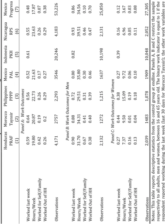
Table 1 provides descriptive statistics for the standardized work variables that we construct across the seven studies, using data from the control group to show work outcomes in the absence of the program.1415
Many of the program recipients would have worked in the absence of the program. Pre-program employment ranged from 48 percent in Mexico Progresa to 64 percent in Morocco, with a weighted mean of 55 percent across all programs. Note that this figures includes all adults aged 16 to 65, including those not in the labor force due to being in school, disability, or retirement. Across everyone regardless of employment status, we observe about 20 hours of work per week, implying about a 40 hour work week for those who are employed.
However, these means mask considerably heterogeneity in work patterns. First, male employment rates are high, with a weighted average of about 87 percent; in contrast, female employment rates tend to be much lower, ranging from 12 percent in Mexico Progresa to 44 percent in Morocco. Second, for most countries, work outcomes tend to be split between self-employment/family work and outside work, with two key exceptions: men in Honduras tend to be more engaged in work inside the house, while men in Mexico’s Progresa program tend to be more engaged in outside work.
14 Note that we provide the control group statistics rather than the baseline since we do not have baseline data for two of the programs and the definitions of work are not the same in the baseline and endline for one of the evaluations (Morocco’s Tayssir).
15Appendix Tables A1 and A2 report the baseline balance check by program, or in the case of the two
programs without baseline, the balance on demographic characteristics at endline. With the exception of PAL and Progresa—for which the analysis in Tables 2-5 uses the difference-in-difference specification—the joint significance tests do not reject balance.
12 IV. DO CASH TRANSFERS REDUCE WORK?
A. OVERALL FINDINGS
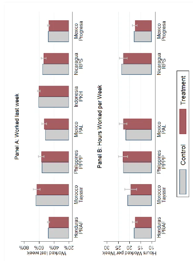
Figure 2 provides a graphical summary of our main findings. In Figure 2A, we graph the employment rate for all eligible adults in both the control and treatment arms for each evaluation. Note that the evaluations are listed in order from the least generous in terms of benefits relative to consumption levels (Honduras’ PRAF) to the most generous (Nicaragua’s RPS and Mexico’s Progresa). Figure 2B replicates Figure 1A, but for hours of work. As one can see by just looking across each program, the overall figures for both employment and hours of work are similar across treatment and control across all of the programs.
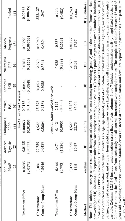
Table 2 provides the corresponding regression analysis underlying Figure 2. Panel A presents the analysis for the employment outcome, while Panel B does so for hours of work per week. Columns 1 through 7 present the analysis for each individual program, while Column 8 provides the pooled analysis for the five programs in which baseline data are also available.
As Figure 2 showed, we do not observe a significant effect of belonging to a transfer program on employment or hours of work in any of the seven programs. Turning to the pooled estimates in Column 8, we also cannot distinguish the effect of the program from zero. These insignificant results are not just driven by large standard errors, as the estimated magnitudes of the pooled treatment effects are, in fact, very small. For example, the coefficient on employed is -.004, representing a statistically insignificant 0.67 percent (i.e., about two thirds of one percent) relative to the control group of 55 percent (p-value of 0.56). The 95% confidence interval on this estimate is between a 1.6 percentage point decrease and a 0.9 percentage point increase in the employment probability.
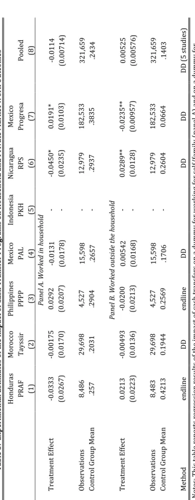
In Table 3, we disaggregate work type by whether the work is self-employed/within family (Panel A) or outside of the household (Panel B). This is especially important if we
13 Figur e 2: E xp eri m enta l E stim ates of Ca sh T ra nsf ers on Work o u tco m es
14 believe that households choose not to work outside the household due to fears that this form of employment could disqualify them from receiving benefits, regardless of whether this fear is rational or irrational according to program rules. Note that we do this for all programs, except Indonesia’s PKH where we do not have the disaggregated data available.
In the four programs that had the least generous benefits (Columns 1-4), we find no statistically observable impacts on either type of work. We find a decrease in outside work and an associated increase in within household work in Mexico’s Progresa program, but the opposite pattern holds for Nicaragua’s RPS program (which has a similar transfer size). Turning to the pooled estimates across the 5 comparable evaluations, we find a 1 percentage point decrease in work within the home (marginally insignificant at the 10 percent level) and no detectable effect on outside work. Thus, overall the results on the allocation of employment are consistent with the zero impact on employment and hours, and mask some heterogeneous impacts going in opposite directions across different programs.
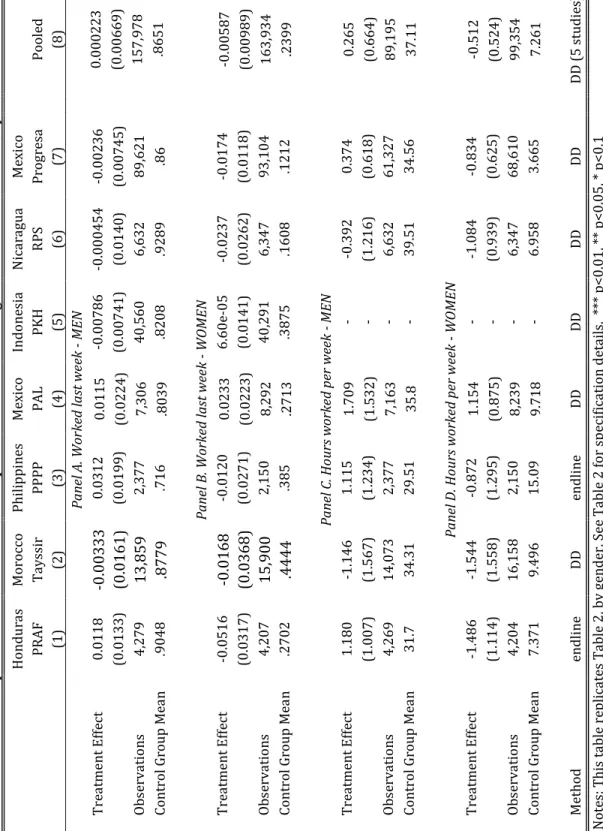
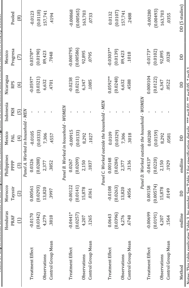
B. DISAGGREGATED BY GENDER
As we observe large differences in baseline employment status across men and women, we next disaggregate the analysis by gender. It is not clear ex ante whether we would expect larger effects for men or women. For example, the additional income may allow a woman who previously had to work the ability to choose to stay home with the children if she prefers, or the additional income may make it possible for her to afford additional child care and actually work more. Alternatively, the literature often paints a picture of the lazy male in the developing country household, who uses transfer stipends to stay home from work and spend money on cigarettes and alcohol.
15 Table 4 replicates Table 2, but disaggregating by gender, while Table 5 does the same for Table 3. The patterns are similar to the main findings above, with no effect of the transfers on either female or male work outcomes.
VI. COMPARISON WITH ASSET TRANSFER PROGRAMS
Our analysis has focused on cash transfers programs that provide small amounts of money either monthly or quarterly to poor households. However, a policy alternative to cash transfers is an
asset transfer program. This is more of a one-time intervention where the beneficiary gets the
gift of a productive asset or money to buy such an asset, with the idea that they will benefit from the income stream from the asset in the future.
The labor supply effect of this program could be quite different from that of an income transfer because it is a lump sum or a lumpy asset, potentially worth much more than the amounts that the beneficiary household has access to through savings or borrowing. If it is a productive asset (e.g. livestock or tools for a business) that requires household labor—say because the labor is needed to take advantage of this capital and because of transaction cost in the labor market that prevent households from hiring labor, or if the household has labor that is underemployed for the same reasons—the presence of the asset would quite naturally encourage the household to work harder. Labor supply would also increase if the household combines the lump sum with a loan to purchase a consumer durable that complements the asset, but then needs work harder to pay down the loan.
There is now evidence on this from a number of asset transfer programs across the world. One version of the program is the so-called graduation model, developed by BRAC in Bangladesh. Under this model, households, chosen for being the poorest members of poor communities, are given an asset of their choosing (from a set of affordable assets) as well as some training and
16 support, including a small income stipend for a short period of time (no more than six months). An RCT of this program by Bandiera et al. (2015) reports, “After four years, eligible women work 170 fewer hours per year in wage employment (a 26% reduction relative to baseline) and 388 more hours in self-employment (a 92% increase relative to baseline). Hence total annual labor supply increases by an additional 218 hours which represents an increase of 19% relative to baseline.” Another RCT by Banerjee et al. (2015) of this program in six different countries (Ethiopia, Ghana, Honduras, India, Pakistan, Peru), reports that total labor supply across the six sites went up by 10 percent of the control group mean (or about 85 hours a year), two years after the start of the program. Consistent with this, both the Bangladesh study and the multi-country study also find increases in income and consumption of commensurate magnitudes in these households.
There is also evidence from a small number of lump sum cash transfer programs. Blattman et al. (2015) carry out a randomized evaluation of a program where women in Northern Uganda most of whom had never run a business before were given a package comprised of $150 in cash, five days of business training, and ongoing supervision. They find that hours worked per week goes up by a stunning 10 hours, and correspondingly, there is a doubling of new non-farm enterprises and a significant rise in incomes. Blattman (2014) also evaluates the Youth Opportunities Program (YOP), a government program in northern Uganda designed to help unemployed adults become self-employed artisans. The government invited young adults to form groups and prepare proposals for how they would use a grant to train in and start independent trades. Funding was randomly assigned among 535 screened, eligible applicant groups. Successful proposals received one-time unsupervised grants worth $7,500 on average— about $382 per group member, roughly their average annual income. After four years the treatment group had 57% greater capital stocks, 38% higher earnings, and 17% more hours of
17
work than did the control group.
Perhaps not surprisingly, these have a strong and clear positive effect on labor supply, in contrast with the more or less zero effect we find from the income support style cash transfer programs. However, it is very important to note two aspects of these programs. First, all of these programs combined assets (or cash for assets) with training and support, and so the evidence is not yet available as to whether supervision is needed to achieve these increases in work or just the asset transfer would be enough. Moreover, it is likely that labor supply is a complementary input to the asset; for example, a cow or goat needs to be fed and taken care of. Future research is needed to disentangle the various aspects of the programs. Second, in thinking through large-scale implementation across governments, physical assets (and in-kind transfers, in general) are often more expensive to distribute than cash. Moreover, we often observe leakages in the distribution of in-kind goods in many developing countries, with the goods never reaching program beneficiaries. New advances in technologies for distributing cash, such as mobile money, may make it easier to provide cash directly to beneficiaries with both potentially low leakage and low costs. Thus, research into understanding how large-scale physical asset distribution programs fare against these newer ways to distribute cash is also important for policy.
V. CONCLUSION
In recent years, there has been a large growth in safety net programs across the developing world. If anything, we might expect this trend to increase as countries become richer: Chetty and Looney (2006) show that social insurance as a fraction of GDP rises as countries get richer, suggesting an that safety nets may be increasingly important as countries grow.
18 As safety nets have increased, so has the debate about whether they simply discourage work, enabling a “lazy poor.” Aggregating evidence from randomized evaluations of seven cash transfer programs, we find no effects of transfers on work behavior, either for men or women. Moreover, a 2014 review of transfer programs worldwide by Evans and Popova also show no evidence—despite claims in the policy debate—that the transfers induce increases in spending on temptation goods, such alcohol and tobacco. Thus, on net, the available evidence implies cash transfer programs do not induce the “bad” behaviors that are often attributed to them in the policy space.
WORKS CITED
Akresh, Richard, Damien De Walque, and Harounan Kazianga. 2013. "Cash Transfers and Child Schooling: Evidence from a Randomized Evaluation of the Role of Conditionality." World Bank Policy Research Working Paper 6340.
Alatas, Vivi, Abhijit Banerjee, Rema Hanna, Benjamin A. Olken, and Julia Tobias. 2012. "Targeting the Poor: Evidence from a Field Experiment in Indonesia." American Economic Review 102(4): 1206-40. Alzúa, María Laura, Guillermo Cruces, and Laura Ripani. 2013. "Welfare programs and labor supply in developing countries: experimental evidence from Latin America." Journal of Population Economics 26(4): 1255-1284.
American Institutes for Research. 2013. “Zambia’s Child Grant Program: 24 Month Impact Report.” Washington, DC.
Ashenfelter, Orley, and Mark W. Plant. 1990. "Nonparametric estimates of the labor-supply effects of negative income tax programs." Journal of Labor Economics, S396-S415.
Attanasio, Orazio, Erich Battistin, Emla Fitzsimons, and Marcos Vera-Hernandez. 2005. "How
effective are conditional cash transfers? Evidence from Colombia." Institute for Fiscal Studies Briefing
Note.
Baird, Sarah, Craig McIntosh, and Berk Özler. 2011. "Cash or condition? Evidence from a cash transfer experiment." Quarterly Journal of Economics, 126(4): 1709-1753.
Bandiera, Oriana, Robin Burgess, Narayan Das, Selim Gulesci, Imran Rasul, and Munshi Sulaiman. 2013. “Can entrepreneurship programs transform the economic lives of the poor?” IZA Discussion Papers 7386.
Banerjee, Abhijit V., Esther Duflo, Nathanael Goldberg, Dean Karlan, Robert Osei, William Parienté, Jeremy Shapiro, Bram Thuysbaert, and Christopher Udry. 2015. “A Multi-faceted Program Causes
19 Lasting Progress for the Very Poor: Evidence from Six Countries.” Science, 348(6236): 1260799. Barrera-Osorio, Felipe, Marianne Bertrand, Leigh L. Linden, and Francisco Perez-Calle. 2011. "Improving the Design of Conditional Transfer Programs: Evidence from a Randomized Education Experiment in Colombia." American Economic Journal: Applied Economics, 3(2): 167-95.
Benhassine, Najy, Florencia Devoto, Esther Duflo, Pascaline Dupas, and Victor Pouliquen. 2015. "Turning a Shove into a Nudge? A "Labeled Cash Transfer" for Education." American Economic Journal: Economic Policy, 7(3): 86-125.
Blattman, Christopher, Nathan Fiala, and Sebastian Martinez. 2014. “Generating skilled employment in developing countries: Experimental evidence from Uganda.” Quarterly Journal of Economics, 129(2): 697–752.
Blattman, Christopher, Eric Green, Julian Jamison, and Jeannie Annan. 2015. “The returns to microenterprise support among the ultra-poor: A field experiment in post-war Uganda” forthcoming in American Economic Journal: Applied Economics.
Chaudhury, Nazmul, Jed Friedman, and Junko Onishi. 2013. "Philippines conditional cash transfer program impact evaluation 2012." Manila: World Bank Report Number 75533-PH.
Chetty, Raj, and Adam Looney. 2007. "Income risk and the benefits of social insurance: Evidence from Indonesia and the United States." In Fiscal Policy and Management in East Asia, NBER-EASE, Volume 16, 99-121. Chicago: University of Chicago Press.
Covarrubias, Katia, Benjamin Davis, and Paul Winters. 2012. "From protection to production: productive impacts of the Malawi social cash transfer scheme."Journal of Development Effectiveness 4(1): 50-77.
Edmonds, Eric V., and Norbert Schady. 2012. "Poverty Alleviation and Child Labor." American Economic Journal: Economic Policy, 4(4): 100-124.
Evans, David, Stephanie Hausladen, Katrina Kosec, and Natasha Reese. 2014. Community-Based Conditional Cash Transfers in Tanzania: Results from a Randomized Trial. Washington, DC: World Bank Publications.
Fiszbein, Ariel, Norbert Rüdiger Schady, and Francisco HG Ferreira. 2009. Conditional cash transfers:
reducing present and future poverty. World Bank Publications.
Galiani, Sebastian, and Patrick J. McEwan. 2013. "The heterogeneous impact of conditional cash transfers." Journal of Public Economics 103: 85-96.
Gentilini, Ugo, Maddalena Honorati, and Ruslan Yemtsov. 2014. “The state of social safety nets 2014.” Washington, DC : World Bank Group.
Gertler, Paul. 2000. "Final Report: The Impact of Progresa on Health." International Food Policy Research Institute (IFPRI): Food Consumption and Nutrition Division.
Gertler, Paul. 2004. "Do conditional cash transfers improve child health? Evidence from PROGRESA's control randomized experiment." American Economic Review 94(2): 336-341.
20 Gilligan, Daniel O., and Shalini Roy. 2013. "Resources, stimulation, and cognition: How transfer programs and preschool shape cognitive development in Uganda." Washington, DC: International Food Policy Research Institute (IFPRI).
Glewwe, Paul, and Pedro Olinto. 2004. “Evaluating the Impact of Conditional Cash Transfers on Schooling: An Experimental Analysis of Honduras’ PRAF Program.” University of Minnesota Unpublished Manuscript.
Haushofer, Johannes, and Jeremy Shapiro. 2013. "Household response to income changes: Evidence from an unconditional cash transfer program in Kenya." Massachusetts Institute of Technology. Imbens, Guido W., Donald B. Rubin, and Bruce I. Sacerdote. 2001. "Estimating the effect of unearned income on labor earnings, savings, and consumption: Evidence from a survey of lottery players." American Economic Review: 778-794.
Maluccio, John, and Rafael Flores. 2005. “Impact Evaluation of a Conditional Cash Transfer Program the Nicaraguan Red de Protección Social.” Washington, DC: International Food Policy Research Institute (IFPRI) Report 141.
Macours, Karen, Norbert Schady, and Renos Vakis. 2012. "Cash Transfers, Behavioral Changes, and Cognitive Development in Early Childhood: Evidence from a Randomized Experiment." American Economic Journal: Applied Economics, 4(2): 247-73.
Parker, Susan W., and Emmanuel Skoufias. 2000. “The Impact of PROGRESA on Work, Leisure, and Time Allocation.” Washington, DC: International Food Policy Research Institute (IFPRI) Report, October.
Schady, Norbert, and Maria C. Araujo. 2008. “Cash Transfers, Conditions, and School Enrollment in Ecuador.” Economía 8(2): 43–70.
Schultz, Paul. 2004. “School subsidies for the poor: Evaluating the Mexican Progresa poverty program.” Journal of Development Economics 74 (1): 199-250.
Skoufias, Emmanuel, and Vincenzo Di Maro. 2008. "Conditional cash transfers, adult work incentives, and poverty." The Journal of Development Studies 44(7): 935-960.
Skoufias, Emmanuel, Mishel Unar, and Teresa Gonzalez de Cossio. 2013. "The poverty impacts of cash and in-kind transfers: experimental evidence from rural Mexico." Journal of Development Effectiveness 5(4): 401-429.
World Bank Office Jakarta. 2011. "Main findings from the impact evaluation of Indonesia's pilot household conditional cash transfer program." World Bank.
21 Ta bl e 1: D escr ip tive S ta tis tics for N on -P ro gr am A re as Hon du ra s M or oc co Phil ipp in es M exico Ind on es ia N ic ar agua M exico PR A F Ta ys sir PPPP PAL PKH R PS Pr og re sa (1) (2) (3) (4) (5) (6) (7) Pa nel A : W ork O ut com es W or ke d la st we ek 0.59 0.64 0.56 0.52 0.61 0.55 0.48 Hour s/ W ee k 19.80 20.87 22.73 21.63 23.63 17.87 W or ke d for S el f/F amil y 0.42 0.19 0.26 0.17 0.26 0.07 W or ke d Out of H H 0.26 0.2 0.29 0.27 0.29 0.38 Ob se rva tio ns 4,171 2757 2,293 3546 20,246 4,183 53,226 Pa nel B : W ork O ut co m es for M en W or ke d la st we ek 0.90 0.88 0.72 0.80 0.82 0.93 0.86 Hour s/ W ee k 31.70 34.31 29.51 35.80 39.51 34.56 W or ke d for S el f/F amil y 0.67 0.41 0.31 0.30 0.46 0.10 W or ke d Out of H H 0.38 0.40 0.39 0.46 0.47 0.70 Ob se rva tio ns 2,132 1272 1,215 1637 10,198 2,131 25,850 Pa nel C: W or k O ut co m es fo r W om en W or ke d la st we ek 0.27 0.44 0.38 0.27 0.39 0.16 0.12 Hour s/ W ee k 7.37 9.50 15.09 9.72 6.96 3.67 W or ke d for S el f/F amil y 0.16 0.01 0.19 0.06 0.05 0.03 W or ke d Out of H H 0.13 0.04 0.18 0.10 0.11 0.08 Ob se rva tio ns 2,039 1483 1,078 1909 10,048 2,052 27,305 N ote s: Th is ta bl e re por ts d es cr ipt iv e sta tistic s fr om th e con tr ol gr ou p at e ndl in e. Pa ne ls A , B a nd C r es tr ic t the s ampl e re sp ec tiv el y to al l a dul ts , m en a nd wo m en , b et w ee n 16 a nd 65 ye ar s ol d. Th e bin ar y wo rk in dic ator is e qua l to 1 if th e re sp on de nt re po rte d wo rk in g duri ng the l as t we ek ( la st 30 da ys f or M or oc co Ta ys sir ); th e othe r wo rk va ria bl es a re re por te d fo r th e sa m e ti me fr ame .
22 Ta bl e 2: Ex p er imen ta l E st ima tes of t h e Imp act of C as h Tr ansf er P ro gr ams on W or k O u tcom es Hon du ra s M or oc co Phil ipp in es M exico Ind on es ia N ic ar agua M exico PR A F Ta ys sir PPPP PAL PKH R PS Pr og re sa Poo le d (1) (2) (3) (4) (5) (6) (7) (8) Pa nel A. W or ked las t w eek Tr ea tme nt E ff ec t -0.0285 -0.0135 0.00863 0.0135 -0.00441 -0.0161 -0.00895 -0.00368 (0.0171) (0.0231) (0.0185) (0.0156) (0.00848) (0.0166) (0.00765) (0.00635) Ob se rva tio ns 8,486 29,759 4,527 15,598 80,851 12,979 182,940 322,127 Con tr ol G roup M ea n 0.5946 0.6439 0.5604 0.5172 0.6058 0.5541 0.4804 .547 Pa nel B . H ou rs w orke d per w eek Tr ea tme nt E ff ec t -0.466 -1.471 0.112 1.154 - -0.928 -0.337 -0.228 (0.793) (1.336) (0.995) (0.880) - (0.839) (0.513) (0.452) Ob se rva tio ns 8,473 30,235 4,527 15,402 - 12,979 130,127 188,743 Con tr ol G roup M ea n 19.8 20.87 22.73 21.63 - 23.63 17.87 21.63 M ethod en dl in e DD en dl in e DD DD DD DD DD (5 stu di es ) N ote s: This ta bl e re por ts r eg re ss io n re sul ts of the im pa ct of ca sh tr an sfe rs on a du mm y fo r wo rk in g (pa ne l A ) a nd on th e num be r of hou rs w or ke d pe r we ek (pa ne l B ). Col um ns 1 -7 re por t r es ul ts fr om ea ch study se pa ra te ly, a nd c ol um n (8) r epo rts a po ol ed r eg re ss ion ove r 5 stud ie s (Hon dura s PR A F an d Phil ipp in es PP P ar e exc lude d). Th e tr ea tme nt eff ec t is th e co eff ic ie nt on Tr ea tme nt x Fol low -up fo r diff er en ce s-in -di ff er en ce s (D D) , an d the c oe ff ic ie nt on Tr ea tme nt oth er wi se . C on tr ol s ar e age , a ge s qua re d, ye ar s of educ ation , ma rita l s ta tus dummie s (s in gl e, ma rr ie d or w ith pa rtn er , divo rc ed or s epa ra te d, an d wi do w), hou se hol d si ze , a nd s urv ey wa ve fixe d eff ec ts , a s w el l a s dummi es for miss in g va lue s for e ac h co ntr ol va ria bl e. C ol umns 1,2,3,5, 6 in cl ude r an do miza tio n st ra ta fix ed e ff ec ts , c ol umns 4 an d 7 in cl ude r an dom iza tion unit ( vil la ge ) fix ed e ff ec ts , a nd Col umn 8 co nta in s th e fix ed e ff ec ts fr om ea ch stu dy an d al l c on tr ol s in te ra ct ed wi th study du mmi es . Th e sa mpl e is a ll adul ts b et we en 1 6 an d 65 ye ar s ol d, exc ludin g dom es tic wo rk er s. Sta nda rd er ro rs c lus te re d at the r an dom iza tion un it le ve l ar e re por te d in pa re nth es es . * ** p<0.0 1, ** p<0.05, * p<0.1
23 Ta bl e 3: Ex p er imen ta l E st ima tes of t h e Imp act of C as h Tr ansf er P ro gr ams on H ouseh old a nd Pr iva te M ar ket W or k O u tc omes Hon du ra s M or oc co Phil ipp in es M exico Ind on es ia N ic ar agua M exico PR A F Ta ys sir PPPP PAL PKH R PS Pr og re sa Poo le d (1) (2) (3) (4) (5) (6) (7) (8) Pa nel A. W or ked in h ou seh ol d Tr ea tme nt E ff ec t -0.0333 -0.00175 0.0292 -0.0131 - -0.0450* 0.0191* -0.0114 (0.0267) (0.0170) (0.0207) (0.0178) - (0.0235) (0.0103) (0.00714) Ob se rva tio ns 8,486 29,698 4,527 15,598 - 12,979 182,533 321,659 Con tr ol G roup M ea n .257 .2031 .2904 .2657 - .2937 .3835 .2434 Pa nel B . W orke d ou ts id e the hou seho ld Tr ea tme nt E ff ec t 0.0213 -0.00493 -0.0200 0.00542 - 0.0289* * -0.0235* * 0.00525 (0.0223) (0.0136) (0.0213) (0.0168) - (0.0128) (0.00957) (0.00576) Ob se rva tio ns 8,483 29,698 4,527 15,598 - 12,979 182,533 321,659 Con tr ol G roup M ea n 0.4213 0.1944 0.2569 .1706 - 0.2604 0.0664 .1403 M ethod en dl in e DD en dl in e DD DD DD DD (5 stu di es ) N ote s: T his ta bl e re po rts r eg re ss io n re sul ts of th e im pa ct of ca sh tr an sfe rs o n a du mm y fo r wo rk in g fo r se lf/fa mil y (pa ne l A ) an d on a dummy for wo rk in g ou ts ide th e hou se hol d (pa ne l B ). S ee Ta bl e 2 no te s fo r sp ec ifi ca tio n de ta ils . * ** p<0.0 1, ** p<0.0 5, * p<0.1
24 Ta bl e 4: Ex p er imen ta l E st ima tes of t h e Imp act of C as h Tr ansf er P ro gr ams on W or k O u tcom es, by G ender Hon du ra s M or oc co Phil ipp in es M exico Ind on es ia N ic ar agua M exico PR A F Ta ys sir PPPP PAL PKH R PS Pr og re sa Poo le d (1) (2) (3) (4) (5) (6) (7) (8) Pa nel A. W or ked las t w eek - M EN Tr ea tme nt E ff ec t 0.0118 -0.00 333 0.0312 0.0115 -0.00786 -0.000454 -0.00236 0.000223 (0.0133) (0.0161) (0.0199) (0.0224) (0.00741) (0.0140) (0.00745) (0.00669) Ob se rva tio ns 4,279 13,859 2,377 7,306 40,560 6,632 89,621 157,978 Con tr ol G roup M ea n .9048 .8779 .716 .8039 .8208 .9289 .86 .8651 Pa nel B . W orke d las t w ee k - W O M EN Tr ea tme nt E ff ec t -0.0516 -0.01 68 -0.0120 0.0233 6.60e -05 -0.0237 -0.0174 -0.00587 (0.0317) (0.0368) (0.0271) (0.0223) (0.0141) (0.0262) (0.0118) (0.00989) Ob se rva tio ns 4,207 15,900 2,150 8,292 40,291 6,347 93,104 163,934 Con tr ol G roup M ea n .2702 .4444 .385 .2713 .3875 .1608 .1212 .2399 Pa nel C. H ou rs w orke d per w eek - M EN Tr ea tme nt E ff ec t 1.180 -1.146 1.115 1.709 - -0.392 0.374 0.265 (1.007) (1.567) (1.234) (1.532) - (1.216) (0.618) (0.664) Ob se rva tio ns 4,269 14,073 2,377 7,163 - 6,632 61,327 89,195 Con tr ol G roup M ea n 31.7 34.31 29.51 35.8 - 39.51 34.56 37.11 Pa nel D . H ou rs w orke d per w eek - W O M EN Tr ea tme nt E ff ec t -1.486 -1.544 -0.872 1.154 - -1.084 -0.834 -0.512 (1.114) (1.558) (1.295) (0.875) - (0.939) (0.625) (0.524) Ob se rva tio ns 4,204 16,158 2,150 8,239 - 6,347 68,610 99,354 Con tr ol G roup M ea n 7.371 9.496 15.09 9.718 - 6.958 3.665 7.261 M ethod en dl in e DD en dl in e DD DD DD DD DD (5 stu di es ) N ote s: T his ta bl e re pl ic ate s Ta bl e 2, by g en de r. Se e Ta bl e 2 for s pe cifi ca tion d eta ils . ** * p<0.01, * * p<0.05, * p<0. 1
25 Ta bl e 5: Ex p er imen ta l E st ima tes of t h e Imp act of C as h Tr ansf er P ro gr ams on H ouseh old a nd Pr iva te Ma rket W or k, by G end er Hon du ra s M or oc co Phil ipp in es M exico Ind on es ia N ic ar agua M exico PR A F Ta ys sir PPPP PAL PKH R PS Pr og re sa Poo le d (1) (2) (3) (4) (5) (6) (7) (8) Pa nel A. W or ked in h ou seh ol d - M EN Tr ea tme nt E ff ec t -0.0170 0.00561 0.0326 -0.0105 - -0.0597* 0.0378* * -0.0123 (0.0342) (0.0293) (0.0288) (0.0333) - (0.0321) (0.0190) (0.0118) Ob se rva tio ns 4,279 13,820 2,377 7,306 - 6,632 89,423 157,741 Con tr ol G roup M ea n .3818 .3997 .3852 .4557 - .4701 .7048 .4194 Pa nel B . W orke d in ho us eho ld - W O M EN Tr ea tme nt E ff ec t -0.0441* -0.00122 0.0267 -0.00915 - -0.0238 -0.000795 -0.00868 (0.0257) (0.0141) (0.0209) (0.0133) - (0.0211) (0.00586) (0.00565) Ob se rva tio ns 4,207 15,878 2,150 8,292 - 6,347 92,895 163,703 Con tr ol G roup M ea n .1265 .0361 .1837 .1027 - .1085 .0795 .0733 Pa nel C. W or ked o ut si de the hou seho ld - M EN Tr ea tme nt E ff ec t 0.0643 -0.0108 0.00148 0.0109 - 0.0592* * -0.0303* * 0.0132 (0.0396) (0.0263) (0.0284) (0.0329) - (0.0248) (0.0139) (0.0107) Ob se rva tio ns 4,276 13,820 2,377 7,306 - 6,632 89,423 157,741 Con tr ol G roup M ea n .6748 .4056 .3136 .3018 - .4588 .1018 .2488 Pa nel D . W or ked ou ts id e the hou seho ld - W O M EN Tr ea tme nt E ff ec t -0.00699 0.00158 -0.0413* 0.00200 - 0.000104 -0.0173* -0.00280 (0.0191) (0.00574) (0.0220) (0.0159) - (0.0122) (0.0102) (0.00493) Ob se rva tio ns 4,207 15,878 2,150 8,292 - 6,347 92,895 163,703 Con tr ol G roup M ea n .1564 .0149 .1929 .0581 - .0522 .0328 .0355 M ethod en dl in e DD en dl in e DD DD DD DD (5 stu di es ) N ote s: T his ta bl e re pl ic ate s Ta bl e 3, by g en de r. Se e Ta bl e 2 for s pe cifi ca tion d eta ils . ** * p<0.01, * * p<0.05, * p<0. 1
26 Appe n dix Tab le 1 A: Bal ance C heck Hon d u ra s PR AF Mo rocco T ayss ir Ph il ip p ine s PPP Ctl Tr ea t Diff Ctl Tr ea t Diff Ctl Tr ea t Diff Pa nel A : D em og ra phi c Cha ra ct er is ti cs o f I nd ivi du als Ag e 1 6-65 Ma le 0.51 0.50 -0.01 0.48 0.48 0.00 0.53 0.52 -0.01 (0.01) (0.01) (0.01) A ge 33.47 33.58 0.11 34.53 34.49 -0.00 33.07 32.84 -0.27 (0.32) (0.23) (0.30) Ye ar s of Ed uc ation 3.07 3.41 0.35* 1.59 1.60 0.03 6.32 6.35 0.10 (0.19) (0.10) (0.20) M ar rie d 0.65 0.65 -0.00 0.60 0.60 -0.00 (0.01) (0.02) Divor ce d 0.01 0.00 0.00 0.01 0.01 -0.00 (0.00) (0.00) W ido w 0.03 0.03 0.01* (0.01) Sin gl e 0.32 0.32 0.00 0.37 0.36 -0.01 (0.01) (0.02) # P eo pl e in H H 5.61 5.81 0.19 6.64 6.57 -0.03 6.04 6.13 0.09 (0.13) (0.09) (0.13) P-va lue , joi nt sig nifi ca nc e 0.14 0.94 0.38 Pa nel B : W ork in g Va ri abl es for I nd iv id ua ls Age 16 -65 (C on troll in g for D em og ra ph ic Ch ara ct er is ti cs ) W or ke d La st W ee k 0.39 0.39 -0.00 (0.01) Hour s W or ke d Pe r W ee k 47.04 47.88 0.63 (0.81) W or ke d Fo r Se lf/F amil y 0.14 0.14 -0.01 (0.01) W or ke d Out of H H 0.25 0.25 0.00 (0.01) P-va lue , joi nt sig nifi ca nc e 0.72 N ote s: T his ta bl e re por ts th e re sul ts o f a b al an ce c he ck b etw ee n tr ea tme nt a nd c on tr ol fo r ea ch stu dy sa m pl e. Da ta for PR A F an d PPP c om e fr om en dl in e; da ta fr om al l oth er p rogr am s come fr om b as el in e. F or e ac h pr og ra m, the c ol umn “C tl ” is me an in c on tr ol a re as , “T re at” is m ea n in t re at me nt ar ea s, an d “Dif f” is dif fe re nc e be tw ee n tr ea tme nt an d con tr ol , c on tr ol lin g for s tr ata fix ed eff ec ts ( for a ll pr og ra ms b ut PA L an d Pr ogr es a) , wi th sta nda rd er ror s cl us te re d at th e ra nd omiza ti on u nit. In Pa ne l B , “ Diff ” a ls o con tr ol s fo r de m ogr aph ic v ar ia bl es . The p -va lue fr om a join t t es t of d emog ra phic ( Pa ne l A ) an d wo rk in g (Pa ne l B ) va ria bl es for e ac h p rogr am is p rovi de d wh en poss ib le .
27 Appe n dix Tab le 1 B: Ba lance C heck , Co n ti n ued M exico PAL Ind on es ia P KH N ic ar agua R PS M exico Pr ogr es a Ctl Tr ea t Diff Ctl Tr ea t Diff Ctl Tr ea t Diff Ctl Tr ea t Diff Pa nel A : D em og ra phi c Cha ra ct er is ti cs o f I nd ivi du als Ag e 1 6-65 Ma le 0.47 0.48 0.01 0.50 0.50 0.00 0.52 0.52 0.00 0.49 0.49 0.01* (0.01) (0.00) (0.01) (0.00) A ge 34.51 35.02 0.51 35.24 35.20 -0.04 32.07 31.91 -0.14 34.04 33.87 -0.17 (0.47) (0.10) (0.32) (0.24) Ye ar s of Ed uc ation 5.26 5.02 -0.24 5.88 5.81 -0.09 2.34 2.18 -0.25 3.66 3.65 -0.01 (0.29) (0.07) (0.19) (0.13) M ar rie d 0.69 0.68 -0.00 0.76 0.76 0.00 0.61 0.63 0.02 0.69 0.68 -0.00 (0.02) (0.01) (0.02) (0.01) Divor ce d 0.04 0.03 -0.00 0.01 0.01 -0.00 0.05 0.06 0.01 0.02 0.02 -0.00 (0.01) (0.00) (0.01) (0.00) W ido w 0.03 0.03 -0.01 0.04 0.04 -0.00 0.02 0.02 -0.00 0.04 0.04 -0.00 (0.00) (0.00) (0.00) (0.00) Sin gl e 0.24 0.26 0.02 0.18 0.19 0.00 0.31 0.29 -0.03* 0.25 0.26 0.01 (0.01) (0.01) (0.01) (0.01) # P eo pl e in H H 4.74 4.64 -0.10 5.16 5.12 -0.05 6.22 6.05 -0.14 5.61 5.60 -0.01 (0.18) (0.04) (0.14) (0.07) P-va lue , joi nt sig nifi ca nc e 0.33 0.41 0.58 0.24 Pa nel B : W ork in g Va ri abl es for I nd iv id ua ls Age 16 -65 (C on troll in g for D em og ra ph ic Ch ara ct er is ti cs ) W or ke d La st W ee k 0.51 0.51 -0.00 0.59 0.59 -0.00 0.58 0.58 -0.00 0.51 0.53 0.02* * (0.02) (0.01) (0.02) (0.01) Hour s W or ke d Pe r W ee k 22.84 21.12 -1.85* 23.81 23.49 -0.43 22.34 22.96 0.44 (0.97) (0.84) (0.49) W or ke d Fo r Se lf/F amil y 0.23 0.25 0.02 0.27 0.25 -0.02 0.10 0.14 0.04* ** (0.03) (0.02) (0.01) W or ke d Out of H H 0.28 0.26 -0.02 0.31 0.33 0.02 0.38 0.35 -0.03* * (0.03) (0.03) (0.01) P-va lue , joi nt sig nifi ca nc e 0.04 0.62 0.01 N ote s: T his ta bl e re por ts th e re sul ts o f a b al an ce c he ck b etw ee n tr ea tme nt a nd c on tr ol fo r ea ch stu dy sa m pl e. Da ta for PR A F an d PPP c om e fr om en dl in e; da ta fr om al l oth er p rogr am s come fr om b as el in e. F or e ac h pr og ra m, the c ol umn “C tl ” is me an in c on tr ol a re as , “T re at” is m ea n in t re at me nt ar ea s, an d “Dif f” is dif fe re nc e be tw ee n tr ea tme nt an d con tr ol , c on tr ol lin g for s tr ata fix ed eff ec ts ( for a ll pr og ra ms b ut PA L an d Pr ogr es a) , wi th sta nda rd er ror s cl us te re d at th e ra nd omiza ti on u nit. In Pa ne l B , “ Diff ” a ls o con tr ol s fo r de m ogr aph ic v ar ia bl es . The p -va lue fr om a join t t es t of d emog ra phic ( Pa ne l A ) an d wo rk in g (Pa ne l B ) va ria bl es for e ac h p rogr am is p rovi de d wh en poss ib le .
28
Program Notes for Honduras PRAF
Data Source. Endline survey data from Glewwe and Olinto (2004); treatment and randomization
strata from Galiani and McEwan (2013).
Program Eligibility. The 70 poorest municipalities in Honduras were eligible for PRAF16. Within eligible municipalities, households with pregnant women or children younger than three were eligible for the health transfer, and households with children 6-12 enrolled in grade 1-4 were eligible for the education transfer.
Original Study Randomization. 70 municipalities were grouped into five strata based on their mean
height-for-age z-score for first graders. Within each stratum, four municipalities were randomly assigned to receive CCTs, four to receive CCTs plus direct investments in health and education, two to receive direct investments only, and four to control. Randomization occurred publically.
Original Study Sample. Within each municipality, 8 communities were randomly selected, and 10
dwellings (which could contain multiple households) were randomly selected to be interviewed at baseline. The endline sample consists of 92% of the 5,748 households from baseline. Additionally, household members who left their baseline household were followed if they were pregnant women, lactating mothers, or children age 0-16.
Sample restriction. We restrict to municipalities assigned to CCTs only or control. We restrict to
adults between 16 and 65 at the time of the survey. Individuals defined as the household’s domestic workers are dropped from the sample (57 observations).
Variable Definitions. The household roster asks whether each member worked in the last week for
a private job and if each member worked in the last week for self/family. Household members are also asked for the work activity to which they dedicated the most time last week, the days spent working on this activity, and the hours per day spent working on this activity.
We code the “Worked last week” dummy is equal to 1 if the household member reports working in a private job, working for self/family, or working 1-7 days on a work activity. The “Worked for Self/Family” dummy is equal to 1 if the household member reports working for self/family, and the “Worked Out of HH” dummy is equal to 1 if the household member reports working for a private job. “Hours per week” is obtained by multiplying hours per day and days per week, censoring at 98 hours per week, and filling with zero if the individual did not work.
We code age, gender, and years of education, as well as household size, from the household roster.
Other notes. We do not use baseline data from PRAF because treatment and control areas were
interviewed in different coffee growing seasons, which influences labor.
16 298 municipalities were sorted based on mean height-for-age z-score for first graders; eligible municipalities had a z-score below the cutoff od -2.304. Three municipalities were excluded because of distance and cost, leaving a final sample of 70 municipalities.
29
Program Notes for Morocco Tayssir
Data Source. Data from Benhassine, Devoto, Duflo, Dupas, and Pouliquen (2015). Program Eligibility. All households in treatment school sectors were eligible.
Original Study Randomization. 314 school sectors were randomized into control (59 sectors) and
treatment (255), stratified by 46 regions.
Original Study Sample. In each school cluster, 6 households were randomly selected from a list of
households in the school's vicinity that had at least one child enrolled in school, and 2 households were randomly selected from a list of households with no child currently enrolled in school but at least one child of school-age who had enrolled at some point but dropped out within the previous three years.
Sample restriction. We restrict to adults between 16 and 65 at the time of the survey. No domestic
workers appear in the original sample.
Variable Definitions. There are two types of question on work activities. The household roster asks
the main activity of each member during the past 30 days, with the following options: (1) worked throughout the period as self-employed, (2) was employed throughout the period, (3) worked occasionally, (4) was looking for work, (5) domestic tasks, (6) studied, (7) was sick, (8) is retired, (9) did not work, (10) other.
Another section asks about the top three paid and unpaid work activities during the past 30 days. It contains questions on the number of day in the past 30 days, and the average number of hours per working day in this activity. In the baseline survey domestic tasks is included as one of the work activities, and this option disappears for the baseline.
We code the “Worked last week” dummy is equal to 1 for options 1, 2 and 3 of the first question (main activity). In addition, at endline only, we code it as 1 if the person reported positive hours in the section on work activities.17 The “Worked for Self/Family” dummy is equal to 1 for options 1, and the “Worked Out of HH” dummy is equal to 1 for options 2 and 3. Hours of work per month are calculated using the top three work activities, multiplying days in the past 30 days and hours per day worked, and summing up over the top three activities. “Hours per week” is obtained by multiplying by 7/30 and censoring at 98 hours per week.
We code age, gender, years of education and marital status, as well as household size, from the household roster.
Other notes. Years of education is asked for persons above 15 years and 17 years at baseline and
endline, respectively. Thus, we are missing this data for 16 year olds at endline.
17 At baseline, 88% of adult women reported at least one activity – this includes domestic tasks. By comparison, 44% of adult women reported a work activity at endline, when domestic tasks was no longer an option. For other programs we do not code domestic tasks as work, hence we decided to use only the main reported activity at baseline. This leads to classifying 3% of women as working at baseline, and 44% at endline. For men, these numbers are 78% and 87%.
30
Program Notes for Philippines PPPP
Data Source. Data from Chaudhury, Friedman and Onishi (2013).
Program Eligibility. Beneficiaries were selected using a combination of geographical targeting and
proxy means testing (PMT), using data from the National Household Targeting System for Poverty Reduction (NHTS-PR). Households are eligible if they have a pregnant mother at the time of the Household Assessment by NHTS-PR and/or children between 0-14 years of age.
Original Study Randomization. 130 villages (barangay) were randomized into 65 treatment and
65 control villages, stratified by 8 municipalities.
Original Study Sample. The original study included 4 sample groups.
Sample restriction. We first restrict attention to sample group 1, namely 10 random eligible
households in each study village. We restrict to adults between 16 and 65 at the time of the survey.
Variable Definitions. The survey contains a question on the whether the respondent did any work
or business at least one hour during the past 7 days. This is our “Worked last week” dummy. A follow-up question asks the sector of work, with options: (0) worked for private household, (1) worked for private establishment, (2) work for government corporation, (3) self-employed without any paid employee, (4) employer in own family-operated farm or business, (5) worked with pay on own family-operated farm or business, (6) worked without pay on own family-operated farm or business, (8) don't know, (9) no response. The “Worked for Self/Family” dummy is equal to 1 for options 3, 4, 5 and 6, and the “Worked Out of HH” dummy is equal to 1 for options 0, 1 and 2. We use a follow-up question on the total number of hours from all jobs during the past 7 days to calculate the “Hours per week” variable, which we top code at 98 hours per week.
We code age, gender, years of education and marital status, as well as household size, from the household roster.
Program Notes for Mexico PAL
Data Source. Data from Cunha, De Giorgi, and Jayachandran (2013).
Program Eligibility. Poor households in eligible localities18 (around 89% of sample population); however, household targeting was not implemented, implying all households in treated localities received PAL.
Original Study Randomization. 208 localities in eight states in southern Mexico were randomized
into one of three treatments (25% of localities each to in-kind transfer treatment, in-kind transfer
18 Villages are eligible for PAL if they have fewer than 2,500 inhabitants, are highly marginalized (classified by Census Bureau), and do not receive aid from Liconsa (subsidized milk program) or Oportunidades (CCT that originated as Progresa). PAL villages tend to be poorer and more rural than Progresa villages.