HAL Id: hal-01313615
https://hal.archives-ouvertes.fr/hal-01313615
Submitted on 11 May 2016
HAL is a multi-disciplinary open access
archive for the deposit and dissemination of
sci-entific research documents, whether they are
pub-lished or not. The documents may come from
teaching and research institutions in France or
abroad, or from public or private research centers.
L’archive ouverte pluridisciplinaire HAL, est
destinée au dépôt et à la diffusion de documents
scientifiques de niveau recherche, publiés ou non,
émanant des établissements d’enseignement et de
recherche français ou étrangers, des laboratoires
publics ou privés.
Abnormal Ventricular Electrograms
Rocío Cabrera-Lozoya, Benjamin Berte, Hubert Cochet, Pierre Jaïs, Nicholas
Ayache, Maxime Sermesant
To cite this version:
Rocío Cabrera-Lozoya, Benjamin Berte, Hubert Cochet, Pierre Jaïs, Nicholas Ayache, et al..
Image-based Biophysical Simulation of Intracardiac Abnormal Ventricular Electrograms. IEEE
Transac-tions on Biomedical Engineering, Institute of Electrical and Electronics Engineers, 2016, PP (99),
�10.1109/TBME.2016.2562918�. �hal-01313615�
Intracardiac Abnormal Ventricular Electrograms
Roc´ıo Cabrera-Lozoya, Benjamin Berte, Hubert Cochet, Pierre Ja¨ıs, Nicholas Ayache, Maxime Sermesant
Abstract— Goal: In this work, we used in silico patient-specific models constructed from 3D delayed-enhanced magnetic resonance imaging (DE-MRI) to simulate intracardiac electro-grams (EGM). These included electrically abnormal electroelectro-grams as these are potential radiofrequency ablation (RFA) targets. Methods: We generated signals with distinguishable macroscopic normal and abnormal characteristics by constructing MRI-based patient-specific structural heart models and by solving the simplified biophysical Mitchell-Schaeffer model of cardiac electrophysiology. Then, we simulated intracardiac electrograms by modelling a recording catheter using a dipole approach. Results: Qualitative results show that simulated EGM resemble clinical signals. Additionally, the quantitative assessment of signal features extracted from the simulated EGM showed statistically significant differences (p<0.0001) between the distributions of normal and abnormal electrograms, similarly to what is observed on clinical data. Conclusion: We demonstrate the feasibility of coupling simplified cardiac EP models with imaging data to generate intracardiac EMG. Significance: These results are a step forward in the direction of the pre-operative and non-invasive identification of ablation targets to guide RFA therapy.
Index Terms—cardiac electrophysiology modelling, intracar-diac electrogram modelling, radiofrequency ablation planning, electroanatomical mapping.
I. INTRODUCTION
D
Espite its numerous advantages over the implantation of a defibrillator, radiofrequency ablation as a curative therapy for patients at risk of sudden cardiac death is still challenging due to the difficulty in finding the appropriate ablation targets. Invasive measures of cardiac activity obtained during an electrophysiology (EP) study provide insightful information about the electrical characteristics of the analysed myocardium. Under pathological conditions, these extracellu-lar recordings deviate from the normal (healthy) signal shape and present multiple deflections and fractionation episodes. However, this lengthy and invasive procedure is difficult for both the patient and the clinician. This is why we are exploring non-invasive approaches to define the ablation targets pre-operatively.In this work, we focus on a target that recently emerged as an appropriate therapy. On structurally diseased hearts with fibrotic scar, bundles of surviving tissue promote electrical circuit re-entry and are a cause of arrhythmias. Local abnormal ventricular activities (LAVA) are sharp fractionated bipolar potentials occurring during or after the far-field electrogram. They have been shown to indicate surviving fibers within the
R. Cabrera-Lozoya, N. Ayache and M. Sermesant are with Inria, Asclepios Research Group, Sophia-Antipolis, France
B. Berte, H. Cochet and P. Ja¨ıs are with the IHU Liryc, Hˆopital Cardi-ologique du Haut-L´evˆeque, Bordeaux, France
scar and have been successfully used as targets for radiofre-quency ablation [1].
Previously, fractionated electrograms (EGM) were thought to be caused mainly by artifacts related to the electronics of the acquisition system. Although artifacts indeed may cause complex EGM, most of them are caused by the peculiar behavior of activation fronts, due to structural and electrical complexity of the underlying tissue [2]. Previous studies have used synthetically generated EGM to explore different pathological phenomena. The authors in [3] describe the generation of EGM fractionation from changes in activation wavefront curvature in experimental canine infarction. In [4], the modelling of intracardiac recordings was used to aid in the reconstruction of cardiac ischemia. The work in [5] studied the influence of different catheter angles, locations and filter settings on the morphology of simulated intracardiac EGM and compared them to clinical signals. The study in [6] derived a way to estimate wave direction and conduction velocity from simulated intracardiac EGM recorded using circular mapping catheters and the one in [7] complemented it by applying such estimations on personalized models.
Delayed-enhanced magnetic resonance imaging (DE-MRI) enables a non-invasive 3D assessment of scar topology and heterogeneity with millimetric spatial resolution. It has been hypothesized that areas of intermediate signal intensity in DE-MRI, also referred to as the border zone (BZ), host scarred and surviving myocardium related to arrhythmia in ischemic populations [1].
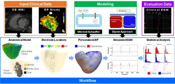
In this work, we test the feasibility of using DE-MR image-based simulation to reproduce macroscopic abnormal patterns in intracardiac EGM. Through this work, we aim to shine some light on the understanding of the macroscopic mechanisms underlying EGM fractionation in the border zone. The overall scheme of the approach is described in Fig. 1.
II. CLINICALDATA
Five patients referred for cardiac ablation of post-infarction ventricular tachycardia (VT) were included in this study. All patients gave written informed consent. They underwent cardiac MRI prior to high-density EP contact mapping of the endocardium (Fig. 1).
A. Imaging Data
The scar tissue was imaged on a 1.5 Tesla clinical device (Avanto, Siemens Medical Systems) 15 minutes after the injection of a gadolinium contrast agent. A whole heart image
Fig. 1: The processing pipeline includes the generation of a personalized cardiac model from imaging data, the simulation of cardiac electrophysiology and intracardiac electrograms and the statistical analysis of the clinical and simulated signals.
was acquired using an inversion-recovery prepared, ECG-gated, respiratory-naviECG-gated, 3D gradient-echo pulse sequence with fat-saturation (1.25×1.25×2.5mm3).
The myocardium was manually segmented on images which were reformatted to have isotropic voxel size (0.625mm3).
Abnormal myocardium consisting of dense scar and border zone areas was segmented using adaptive thresholding of the histogram, with a cut-off at 35% of maximal signal intensity. Segmentations were reviewed by an experienced radiologist, with the option of manual correction.
B. Electrophysiological Data
The CARTO mapping system (Biosense Webster) enables the 3D localization of the catheter tip and provides the dis-tribution of EP signals on cardiac surfaces. Contact mapping was achieved in sinus rhythm on the endocardium (trans-septal approach) with a multi-spline catheter (PentaRay, Biosense Webster). The catheter’s five-branched star design (including 20 electrodes located along 5 branches) allows for high density mapping by recording multiple locations at once. Recordings are of 2.5 seconds of duration. Signals were categorized as normal or abnormal by an experienced electrophysiologist. Table I includes details on the EP studies for each patient.
TABLE I: CARTO Electrophysiology Study Details
P1 P2 P3 P4 P5 µ ± σ # of Catheter Locations 368 1201 339 214 700 567±399 # of Abnormal EGM 71 44 82 44 33 55±21 # of Normal EGM 297 1157 257 170 667 510±409 % of Abnormal EGM 19 4 24 21 5 15±9
Fig. 2 provides further insight in the distribution of the clinical annotations of the electrode locations for Patient 1. The distance to the border zone is computed by taking the Euclidean distance from the annotated signal location to the
closest edge or point in the mesh generated from the border zone segmentation, as will be detailed in Section III-A. If points are within the border zone mesh, their distance is set to zero. Because the distances are computed using a border zone mesh and not the image intensities themselves, the edges of the BZ are not diffuse. It can be seen that abnormal signals have a higher tendency to remain close to the border zone, nonetheless, healthy signals can also be found in these regions. Similar abnormal EGM distributions were found in the remaining four patients.
Fig. 2: (Left) Image-driven personalized model and location of abnormal (red) and normal (blue) annotated signals on Patient 1. (Right) Boxplots representing the distance of the annotated signals to the border zone.
III. CARDIACMODELCONSTRUCTION
Fig. 1 shows our processing pipeline. It consists of the generation of a patient-specific cardiac model from imaging data, with inclusion of synthetic myocardial fibers. A cardiac EP model with tissue-specific properties is solved on this geometry and intracardiac EGM are computed at locations obtained from the clinical EP study. Signal feature extraction is performed on both clinical and simulated EGM, which allows us to perform statistical analysis. Each segment of the pipeline will be detailed in the following sections.
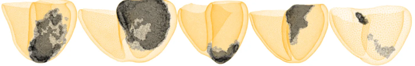
Fig. 3: Personalized heart meshes for our five patients depicting healthy myocardium (yellow), scar (black) and border zone (grey) tissues derived from DE-MRI segmentations.
A. Anatomical Model Generation
Segmentations of the myocardium, border zone and scar regions on DE-MRI were performed using MUSIC software (multimodality software for specific imaging in cardiology, L’Institut de Rythmologie et de Mod´elisation Cardiaque, Uni-versity of Bordeaux, Institut National de Recherche en Infor-matique et AutoInfor-matique Sophia Antipolis, Sophia Antipolis, France). The software is a solution that was developed in-house and built on the open-source medInria software ar-chitecture (http://med.inria.fr). Segmentations masks were the basis to generate personalized 3D tetrahedral meshes of the biventricular myocardium using the CGAL library [8]. Mesh details including mean edge length and number of tetrahedra are shown in Table III.
Myocardial fiber directions were created synthetically as proposed in [9]. The elevation angle (measured w.r.t. the short axis plane) was varied from -80◦ on the epicardium to 0◦ at mid-myocardial wall to +80◦ on the endocardium.
B. Electrophysiology (EP) Model
Cardiac electrophysiology can be described through a va-riety of mathematical models [10], [11], [12], [13]. More detailed cell-specific models also exist which aim to describe cell-to-cell variability in the cardiac tissue [14], [15]. These models have evolved in the last decades to better represent physiological phenomena [16], e.g. some have been used to study VT or other arrhythmia episodes [17], [18], [19], [20].
We chose a model able to represent complex cardiac elec-trical phenomena while keeping the number and variation of the involved variables tractable: the Mitchell-Schaeffer (MS) [13] model. Its main advantages include:
- its simplicity, as it only includes two differential equa-tions
- the relationship between its parameters and physiologi-cal behavior makes it easier to interpret
- its ability to simulate arrhythmia macroscopically due to its restitution parameters
It has been used for patient-specific personalization for VT simulation [19] and interactive simulation of patient-specific EP [21].
The Mitchell-Schaeffer (MS) model describes the trans-membrane potential as the sum of a passive diffusive current and active reactive currents (inward and outward ionic cur-rents). The system of equations used is the following:
∂tu = div(D∇u) +zu 2(1−u) τin − u τout + Jstim(t) ∂tz = ( (1−z) τopen if u < ugate −z τclose if u > ugate (1) Where:
- u: normalised transmembrane potential variable - z: gating variable depicting depolarization and
repolar-ization phases by opening and closing the current gates - Jin = zu2(1 − u)/τin: inward N a+ and Ca2+ ionic
currents which raise the action potential voltage - Jout = u/τout: outward ionic K+ current which
de-creases the action potential voltage during repolarization - Jstim: stimulation current at the pacing location
- τin, τout, τopen, τclose have units of seconds
- D = d · diag(1, r, r): anisotropic diffusion tensor in fiber coordinates which enables conduction velocity in the fiber direction to be 2.5 larger than in the transverse plane (r = 1/2.52)
This model incorporates both action potential duration (APD) and conduction velocity restitution effects. We used the MS model implementation in the SOFA framework [21]. C. Pseudo-personalization: Tissue-specific EP Properties
The EP properties of the infarcted and border zone tissues differ from those of the healthy myocardium. For the construc-tion of our personalized model, DE-MRI was used to asses the viability of the cardiac tissue. We identified tissue as either healthy myocardium, scar or border zone. Fig. 3 shows the derived volumetric ventricular models for each of our patients. Conductivity in the border zone was decreased by 90% with respect to its value in the healthy myocardium [22]. Studies in infarcted hearts [23] [24] [25] [26] reported variations in ionic currents in the border zone tissue generating action potentials that differ from the healthy myocardium, with:
- 32% lower peak action potential amplitudes - 31% smaller upstroke velocity
- 25% longer action potential duration (APD)
Consequently, in our model, the term Jin= zu2(1 − u)/τin
in (1) was modified to zu2(a − u)/τ
in, where variable a
controls the peak amplitude for the action potential. To obtain a smaller upstroke velocity, τinin the border zone was increased
31% with respect to the value in the healthy tissue.
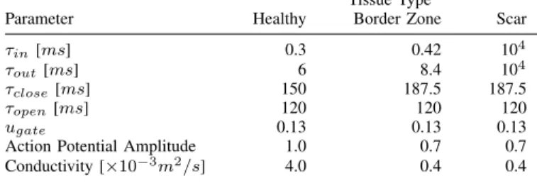
The analytical expression for the maximum APD for the Mitchell-Schaeffer model is given by AP D =
Tissue Type
Parameter Healthy Border Zone Scar
τin[ms] 0.3 0.42 104
τout[ms] 6 8.4 104
τclose[ms] 150 187.5 187.5
τopen[ms] 120 120 120
ugate 0.13 0.13 0.13
Action Potential Amplitude 1.0 0.7 0.7 Conductivity [×10−3m2/s] 4.0 0.4 0.4
τclose ln (τout/4τin), implying a linear relationship between
τcloseand the APD. Therefore, the values for this parameter in
the border zone were increased by 25%. Finally, because τin
had been modified to account for a smaller upstroke velocity, τout was modified in the same proportion to keep the ratio
τout/τin constant.
Scar tissue was modelled to have a null reaction component on the MS model by setting much higher values of τin
and τout with respect to those of the healthy myocardium.
The diffusion component was left with the values of the border zone. Healthy myocardial values were set to the default values in [13]. Furthermore, patient-specific sinus rhythm was extracted from surface electrocardiogram (ECG) recordings. Table II summarizes the parameters used for our personalized simulations.
The current tissue-specific model parameters were not mod-ified to account for the heterogeneity in action potential dura-tions between the endocardial and epicardial [27] nor between the apex to base [28] tissue, which affect the repolarization phase. This study focuses on EGM abnormalities found in the depolarization complex. This can explain the difference between simulated and recorded T-wave patterns.
IV. INTRACARDIACEGM SIMULATION
Extracellular electrograms arise due to transmembrane cur-rents occurring from differences in the axial voltage gradient at the interface between activated and inactivated myocardial cells [2]. If an activation wave front travels from left to right throughout the myocardium, at the boundary of the propagation front, the depolarized cell has an intracellular potential of +20mV whereas that of the cell in resting state remains at -90mV. This creates a current flow from the activated to the inactivated myocyte. To comply with the preservation of charge, the back of the activation front presents a current flow from the extracellular space into the intracellular space, whereas the current flow direction is reversed in the regions ahead of the activation front. This flow of current in the extracellular space generates an extracellular voltage difference and therefore a potential dipole.
A. The Dipole Approach
The notion of resulting dipoles at the depolarization wave front can be used to compute the resulting potential at a given coordinate in the extracellular space [29]. This approach was used by [30] to compute pseudo pre-cordial and limb-lead ECGs from a Purkinje muscle model. We introduce a similar
approach to simulate unipolar and bipolar intracardiac EGM at a given position representing the catheter location.
The monodomain formulation describes the action potential propagation with the following reaction diffusion equation:
Cm
∂v
∂t + Iion= ∇ · σm∇v (2) where v represents the transmembrane potential, Cmis the
membrane capacitance, σm corresponds to the local
conduc-tivity and Iion is the current through the cell membrane per
unit of area. We define the equivalent current density jeq as:
jeq= −σm∇v (3)
−jeq behaves like a flow source density, and it can also be
seen as a dipole moment per unit of volume: p =
Z
jeqdV (4)
According to the volume conductor theory [29], the electric potential registered at a distance R in a homogeneous volume conductor of conductivity σ outside the region occupied by the volume source V is :
Ψ(R) = 1 4πσ Z V jeq· ∇( 1 R)dV (5) In our case, we model the moving propagation front as a local dipole. As this dipole is proportional to the potential gradient, and we use linear elements to solve the model equa-tions, the dipole momentum pX at a position X is spatially
invariant over a single tetrahedron H: ∀X ∈ H, pX= pH.
Then we sum the potential over all the myocardial regions: those being activated, those depolarized and those at rest. Non-activated regions give almost null dipole momenta and it simplifies the overall calculation.
We discretize (4) in space (H tetrahedra of the mesh) and get the formulation of the dipole moment of the charge in the volume VH of tetrahedron H :
pH= VHjeq,Ht = VHσm,H∇vH (6)
The gradient of the electrical potential in the tetrahedron ∇vH is computed using its node values and its shape vectors
as defined in [31], and the dipole is located at the tetrahedron center XH.
From (5), the contribution ΨH(Xel) of tetrahedron H to
the potential field calculated at the electrode location Xel is
estimated by: ΨH(Xel) = 1 4πσ (VHσm,H∇vH) · (Xel− XH) kXel− XHk3 (7) Finally, we sum over the whole mesh to get the potential field at Xel: Ψ(Xel) =P
N b tetra
ploring electrode in the heart and the indifferent electrode away from the heart so it has little or no cardiac signal [32]. Bipolar EGM correspond to the difference in potential between two unipolar measurements and are useful to study the local activities. The far-field signal is assumed to be similar for both unipolar recordings so it is largely filtered out [32].
Each of the five branches of the recording catheter used in the clinical environment has four electrodes named M1, M2, M3 and M4 from the distal to the proximal. Two bipolar recordings are generated from these unipolar measurements: M1-M2 and M3-M4 (Fig. 4). Electrode positions at recording time are given by the CARTO system and its spatial coordi-nates are used to generate our computational measurements, as exemplified in Fig. 1.
Fig. 4: The subtraction of two unipolar measurements gener-ates a bipolar measurement. Here, the M1 and M2 unipolar signals are used to generate the bipolar M1-M2 signal.
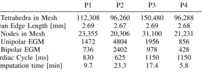
Simulations were performed with a time step of 1 × 10⁻⁵ seconds. Further details on EGM simulations per patient are shown in Table III. Computation times correspond to the sim-ulation of a single cardiac cycle and of all the corresponding patient-specific intracardiac EGM, on a computer with Intel Core i5 CPU.
TABLE III: Patient-specific Simulation Details
P1 P2 P3 P4 P5
# Tetrahedra in Mesh 112,308 96,260 150,480 96,288 29,586 Mean Edge Length [mm] 2.69 2.67 2.69 2.68 3.98 # Nodes in Mesh 23,355 20,306 31,100 21,231 6,742 # Unipolar EGM 1472 4804 1956 856 2800 # Bipolar EGM 736 2402 978 428 1400 Cardiac Cycle [ms] 830 625 1150 1150 830 Computation time [min] 9.7 23.3 17.4 5.8 4.3
V. SIGNALANALYSIS
In addition to a qualitative assessment of signal morphology, a quantitative signal evaluation was performed by extracting the signal characteristics from simulated and clinical EGM.
- Signal Range: difference between the maximum and minimum amplitude signal values.
- Number of Inflection Points: number of points where the signal changes concavity.
- Signal Energy: calculated using Teager’s operator [33]. - Dominant Frequency: from the fast Fourier transform. - Mean Slope: mean absolute value of dV /dt.
- Fractionation Index: number of deflections with an amplitude >0.2mV from the signal baseline.
- Minimum and Maximum Signal Value.
Fig. 5: Illustration of signal features extracted for EGM characterization and quantitative analysis.
Some of these features were inspired by those used clini-cally [34] to characterize EGM associated with atrial fibrilla-tion. Signal range is expected to be smaller in abnormal elec-trograms when compared to healthy ones. On the other hand, the number of inflection points, mean slope and fractionation index are interesting characteristics as their values tend to be higher in abnormal electrograms with multiple deflections and fractionation episodes.
The distributions of the values of each of these char-acteristics in the normal and abnormal signal groups were assessed using the non-parametric Kolmogorov-Smirnov (KS) test, as this test does not assume that data come from a normal distribution [35]. This test compares the cumulative distribution functions of two datasets and computes a p value dependent on the maximum distance between them. It is useful to detect substantial differences in either shape, spread or median between the distributions. A value of p < 0.05 was considered as statistically significant.
VI. RESULTS ANDDISCUSSION
Catheter measurements were simulated using the image-driven personalized heart model at personalized sinus rhythm with the parameters stated in Table II. Resulting EGM were qualitatively compared to their clinical counterparts and fea-tures between normal and abnormal groups were assessed.
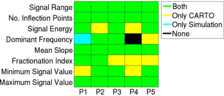
Fig. 7: KS test results. Statistically significant differences (p<0.05) between normal and abnormal feature distributions in (green) both CARTO and simulated signals (yellow) only in CARTO signals (blue) only in simulated signals (black) neither in CARTO nor in simulated signals.
A. Qualitative Assessment of Simulated EGM
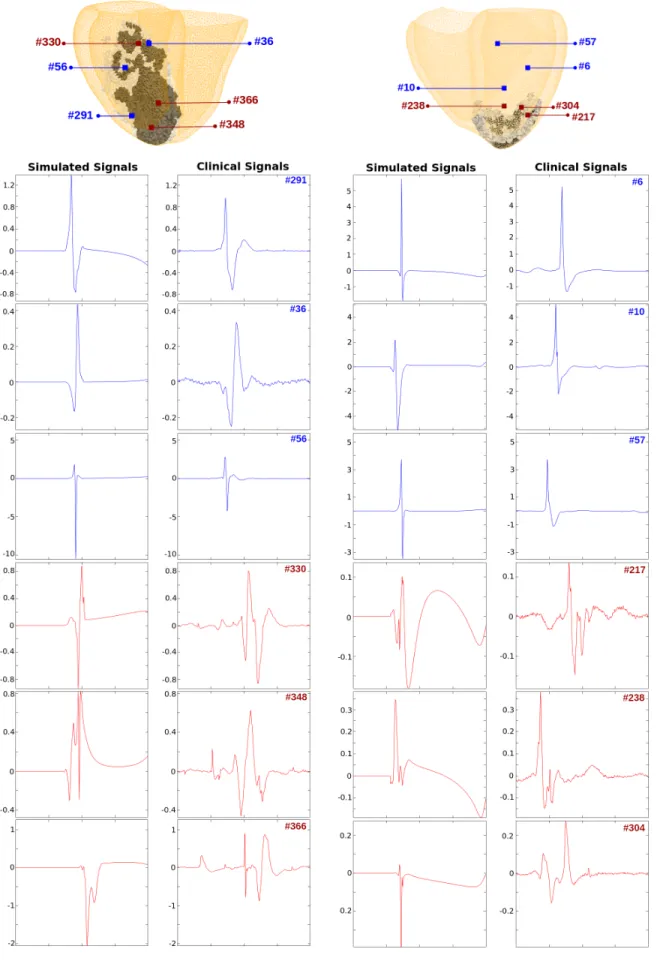
Fig. 6 shows samples of the locations of the electrodes with respect to the cardiac geometry, and the resulting EGM simu-lation and clinical bipolar (M1-M2) signals at these locations for Patients 1 and 3. Three normal and three abnormal signals per patient are depicted.
A first qualitative assessment shows that simulated signals are less prone to noise when compared to the CARTO signals. This is expected as the simulated signals are not affected by catheter movement, breathing or cardiac motion, among other factors.
For the normal simulated signals, we observe a normal ventricular depolarization in the form of a steep slope, without any fragmentation inside the EGM signal. For the abnormal signals, fractionation is found anywhere during the QRS complex of the bipolar EGM.
As was mentioned before, the T-wave abnormality is due to the fact that APD heterogeneity across the myocardium was not accounted for in the model.
B. Clinical and Simulated Signal Characterization
Results of the KS test on the signal characteristics of the clinical CARTO recordings can be obtained from Fig. 7. With the exception of the dominant frequency in Patients 1 and 4, a statistically significant difference between the signal characteristics of normal and abnormal distributions was found. For reference, most test results yielded as low as p value of <0.0001, denoting a very good separability between the class distributions of normal and abnormal signal features. For the simulated signals, the results of the KS test can also be obtained from Fig.7. The distributions of mean slope, number of inflection points and maximum signal value differed significantly among simulated normal and abnormal signal populations, as can be seen by the low p value obtained after the KS test.
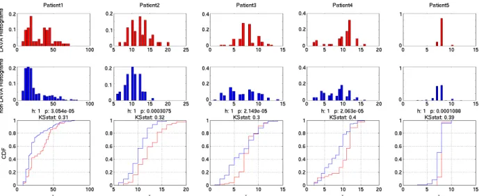
Looking in more detail at these tests, the first two rows in Fig. 8 show the histograms of the distributions for the number of inflection points in the abnormal and normal classes in the simulated signals, respectively. The difference in distributions is perhaps more evident in the bottom row which shows the CDF of both classes. The average KS statistic (maximum
between the distributions.
Figure 7 shows a good agreement between the KS test results in clinical and simulated signals. A statistically signifi-cant difference was found in the distributions of features such as signal range, number of inflection points, mean slope and maximum signal value on both clinical and simulated signals. The distributions of dominant frequency in the signals performed the worst, where a statistically significant difference was only found in simulated signals for Patient 1. For Patient 5, only the CARTO signals had difference in their distribution and no statistically significant difference was found neither in the clinical nor in the simulated signals in Patient 4.
C. Discussion
This exploratory research paper seeks to evaluate whether computer simulation combined with medical imaging is able to pinpoint non-invasively the regions of the myocardium that generate abnormal signals in the same way as it is measured in a clinical environment invasively with a catheter, rather than to recreate EGM signals with high fidelity when compared to their clinical counterparts.
Given all the simplifications in modelling both the biophys-ical phenomenon and the data acquisition procedure, it would be hard to obtain quasi-realistic signals using the approach shown in this paper. Nevertheless, this approach demonstrated statistically significant differences in simulated normal and abnormal intracardiac electrograms which is of high clinical relevance. It opens the door for simulation-based approaches to guide EP interventions in order to guide clinicians to the locations where abnormal electrograms are found. It also restricts the search of abnormalities to subregions in the myocardium and could decrease procedure times. Finally, the clinician would in any case measure the electrical activity in the region before taking the decision of ablating.
VII. CONCLUSION
We presented the use of a personalized image-based model for the simulation of intracardiac EGM with abnormal elec-trical characteristics. We showed that the use of a simpli-fied biophysical electrophysiology model with tissue-specific parameters and the use of a dipole approach to simulate intracardiac electrograms were sufficient to generate abnor-mal signals which are properly localized and distinguishable from their normal counterpart as labeled by an experienced electrophysiologist.
Also, the resemblance of the simulated signals with their clinical CARTO counterpart was qualitatively assessed. Fur-thermore, feature extraction was performed on both the sim-ulated and clinical signals. Characteristics such as the mean slope and number of inflection points presented significantly different distributions when assessed through the use of a Kolmogorov-Smirnov test in both the simulated (p<0.002) and clinical signals (p<0.0001).
The encouraging results obtained in this work demonstrate that it is feasible to generate intracardiac EGM using a
Fig. 8: Histograms of the number of inflection points for abnormal EGM (top) and normal EGM (middle) simulated signals by patient. (bottom) Cumulative distribution functions (CDF) for abnormal EGM (red) and normal EGM (blue) simulated signals.
simplified cardiac EP models personalized with imaging data, with distinct characteristics which could aid in the planning of RFA therapy by pre-operatively and non-invasively identifying ablation targets.
VIII. ACKNOWLEDGEMENT
Part of this work was funded by the European Research Council through the ERC Advanced Grant MedYMA 2011-291080 (on Biophysical Modelling and Analysis of Dynamic Medical Images).
REFERENCES
[1] P. Ja¨ıs, P. Maury, P. Khairy, F. Sacher, I. Nault, Y. Komatsu, M. Hocini, A. Forclaz, A. S. Jadidi, and R. Weerasooryia, “Elimination of local abnormal ventricular activities a new end point for substrate modifica-tion in patients with scar-related ventricular tachycardia,” Circulamodifica-tion, vol. 125, no. 18, pp. 2184–2196, 2012.
[2] J. de Bakker and F. Wittkampf, “The pathophysiologic basis of fraction-ated and complex electrograms and the impact of recording techniques on their detection and interpretation.,” Circulation: Arrhythmia and Electrophysiology, 2010.
[3] E. Ciaccio, H. Ashikaga, J. Coromilas, B. Hopenfeld, D. Cervantes, A. Wit, N. Peters, E. McVeigh, and H. Garan, “Model of bipolar elec-trogram fractionation and conduction block associated with activation wavefront direction at infarct border zone lateral isthmus boundaries.,” Circulation: Arrhythmia and Electrophysiology, 2014.
[4] D. ´Alvarez, F. A. Atienza, J. L. Rojo- ´Alvarez, A. Garc´ıa-Alberola, and M. Moscoso, “Shape reconstruction of cardiac ischemia from non-contact intracardiac recordings: A model study.,” Mathematical and Computer Modelling, vol. 55, no. 5-6, pp. 1770–1781, 2012. [5] M. W. Keller, S. Schuler, A. Luik, G. Seemann, C. Schilling, C. Schmitt,
and O. Dossel, “Comparison of simulated and clinical intracardiac electrograms,” in Engineering in Medicine and Biology Society (EMBC), 2013 35th Annual International Conference of the IEEE, pp. 6858–6861, IEEE, 2013.
[6] F. M. Weber, C. Schilling, G. Seemann, A. Luik, C. Schmitt, C. Lorenz, and O. D¨ossel, “Wave-direction and conduction-velocity analysis from intracardiac electrograms–a single-shot technique,” Biomedical Engi-neering, IEEE Transactions on, vol. 57, no. 10, pp. 2394–2401, 2010. [7] M. Burdumy, A. Luik, P. Neher, R. Hanna, M. W. Krueger, C. Schilling,
H. Barschdorf, C. Lorenz, G. Seemann, C. Schmitt, et al., “Com-paring measured and simulated wave directions in the left atrium–a workflow for model personalization and validation,” Biomedizinische Technik/Biomedical Engineering, vol. 57, no. 2, pp. 79–87, 2012.
[8] T. C. Project, CGAL User and Reference Manual. CGAL Editorial Board, 4.7 ed., 2015.
[9] D. D. Streeter, “Gross morphology and fiber geometry of the heart,” Handbook of physiology, pp. 61–112, 1979.
[10] R. R. Aliev and A. V. Panfilov, “A simple two-variable model of cardiac excitation,” Chaos, Solitons & Fractals, vol. 7, pp. 293–301, Mar. 1996. [11] P. N. K. ten Tusscher, D. Noble and A. Panfilov, “A model for human ventricular tissue,” American Journal of Physiology - Heart and Circulatory Physiology, 2004.
[12] F. Fenton and A. Karma, “Erratum: ”vortex dynamics in three-dimensional continuous myocardium with fiber rotation: Filament insta-bility and fibrillation” [chaos 8, 20-47 (1998)].,” Chaos, vol. 8, p. 879, Dec. 1998.
[13] C. Mitchell and D. Schaeffer., “A two-current model for the dynamics of cardiac membrane.,” Bulletin of Mathematical Biology, 2003. [14] M. Zaniboni, A. E. Pollard, L. Yang, and K. W. Spitzer, “Beat-to-beat
repolarization variability in ventricular myocytes and its suppression by electrical coupling,” American Journal of Physiology-Heart and Circulatory Physiology, vol. 278, no. 3, pp. H677–H687, 2000. [15] A. X. Sarkar, D. J. Christini, and E. A. Sobie, “Exploiting mathematical
models to illuminate electrophysiological variability between individu-als,” The Journal of physiology, vol. 590, no. 11, pp. 2555–2567, 2012. [16] A. E. Pollard, “From myocardial cell models to action potential
propa-gation,” Journal of electrocardiology, vol. 36, pp. 43–49, 2003. [17] M. P. Nash and A. V. Panfilov, “Electromechanical model of excitable
tissue to study reentrant cardiac arrhythmias,” Progress in biophysics and molecular biology, vol. 85, no. 2, pp. 501–522, 2004.
[18] I. V. Kazbanov, R. H. Clayton, M. P. Nash, C. P. Bradley, D. J. Paterson, M. P. Hayward, P. Taggart, and A. V. Panfilov, “Effect of global cardiac ischemia on human ventricular fibrillation: Insights from a multi-scale mechanistic model of the human heart,” 2014.
[19] J. Relan, P. Chinchapatnam, M. Sermesant, K. Rhode, M. Ginks, H. Delingette, C. A. Rinaldi, R. Razavi, and N. Ayache, “Coupled personalization of cardiac electrophysiology models for prediction of ischaemic ventricular tachycardia,” Journal of the Royal Society Inter-face Focus, vol. 1, no. 3, pp. 396–407, 2011.
[20] K. S. McDowell, S. Zahid, F. Vadakkumpadan, J. Blauer, R. S. MacLeod, and N. A. Trayanova, “Virtual electrophysiological study of atrial fibrillation in fibrotic remodeling,” PloS one, vol. 10, no. 2, p. e0117110, 2015.
[21] H. Talbot, S. Marchesseau, C. Duriez, M. Sermesant, S. Cotin, and H. Delingette, “Towards an interactive electromechanical model of the heart,” Interface Focus, vol. 3, no. 2, 2013.
[22] H. Arevalo, G. Plank, P. Helm, H. Halperin, and N. Trayanova, “Tachy-cardia in post-infarction hearts: insights from 3d image-based ventricular models,” PloS one, vol. 8, no. 7, p. e68872, 2013.
[23] K. F. Decker and Y. Rudy, “Ionic mechanisms of electrophysiological heterogeneity and conduction block in the infarct border zone,” Ameri-can Journal of Physiology-Heart and Circulatory Physiology, vol. 299, no. 5, pp. H1588–H1597, 2010.
and Circulatory Physiology, vol. 287, no. 3, pp. H1046–H1054, 2004. [25] M. Jiang, C. Cabo, J.-A. Yao, P. A. Boyden, and G.-N. Tseng, “Delayed
rectifier k currents have reduced amplitudes and altered kinetics in myocytes from infarcted canine ventricle,” Cardiovascular research, vol. 48, no. 1, pp. 34–43, 2000.
[26] J. Pu and P. A. Boyden, “Alterations of na+ currents in myocytes from epicardial border zone of the infarcted heart a possible ionic mechanism for reduced excitability and postrepolarization refractoriness,” Circula-tion Research, vol. 81, no. 1, pp. 110–119, 1997.
[27] C. Antzelevitch and J. Fish, “Electrical heterogeneity within the ven-tricular wall,” Basic research in cardiology, vol. 96, no. 6, pp. 517–527, 2001.
[28] P. C. Franzone, L. Pavarino, S. Scacchi, and B. Taccardi, “Modeling ventricular repolarization: effects of transmural and apex-to-base het-erogeneities in action potential durations,” Mathematical biosciences, vol. 214, no. 1, pp. 140–152, 2008.
[29] J. Malmivuo and R. Plonsey, Bioelectromagnetism: principles and applications of bioelectric and biomagnetic fields. Oxford University Press, 1995.
[30] O. Berenfeld and J. Jalife, “Purkinje-muscle reentry as a mechanism of polymorphic ventricular arrhythmias in a 3-dimensional model of the ventricles,” Circulation Research, 1998.
[31] H. Delingette, “Triangular springs for modeling nonlinear membranes,” IEEE Transactions on Visualization and Computer Graphics, vol. 14, March/April 2008.
[32] W. G. Stevenson and K. Soejima, “Recording techniques for clini-cal electrophysiology,” Journal of Cardiovascular Electrophysiology, vol. 16, no. 9, pp. 1017–1022, 2005.
[33] M. Nguyen, C. Schilling, and O. D¨ossel, “A new approach for automated location of active segments in intracardiac electrograms,” in World Congress on Medical Physics and Biomedical Engineering, September 7-12, 2009, Munich, Germany, pp. 763–766, Springer, 2010.
[34] Y. Takahashi, M. D. ONeill, M. Hocini, R. Dubois, S. Matsuo, S. Knecht, S. Mahapatra, K.-T. Lim, P. Ja¨ıs, A. Jonsson, et al., “Characterization of electrograms associated with termination of chronic atrial fibrillation by catheter ablation,” Journal of the American College of Cardiology, vol. 51, no. 10, pp. 1003–1010, 2008.
[35] J. W. Pratt and J. D. Gibbons, “Kolmogorov-smirnov two-sample tests,” in Concepts of Nonparametric Theory, pp. 318–344, Springer, 1981.