Decomposition methods for facility location problems

-,, _{,,-., ;, -5 , -,. ,---.--} , ,--- , , -;-", ,,,-, _{--iI-' --"-, ,-,-' --., . ,,'Y' - ,,,,, "-,,-,}

-, --- -- -,-,,- --,:- -- , - I- ,- -- ,4

,,-, ,-" ',-,,; -,,,,-',":,.---,"- -',"-,-',,-Z' -- ,.- , ,:,, c , -- ,-,;:- '- ,, -a.- '. -,--- ,,-. i--. ; '- ,.,- _-. 1,,.-

-, .-1 I -, " Z , ., ""-" ,--: " ,

---- ,,-,- -, 7,:,-, ,;J,

I",,,---,3': ,.-.,- -1 ,4F -,. 't, - -! .,.--I, -, .- ,-1I-1 c - III- -.

-I -- ,,---i, 1. -',., ---.- ,,,,--f ;,",', 1'11,--",,---, r,,,--. -- ----, ,., , ,-,: "t-",-.---. .- , .,::, ", -,-- -,,---, 1, --, , I- " w,",, ,,,,---I;?-.-:, -- .- :_,i <sub>-- ,,,1`1 ,I Y 11,.1</sub> - , --,,,-,'. ,-, . ,j,, ' ' -- ,., -,,, ,,-,- ,,,;--- -',,'. t -, , , ,-"-. ,,-.-,,- , -,- 7 --,U ,,--, -- ; -! , - -,-,, -, ,,, , ;- ,-,7---,, ,-, ,-,,, " ': I.,,-,--,-I,- ,,--;- ,-, ,. ,, --,1.,- ,-,.,-, - --- " I I, ,--,-,, -- ,---A- - -,,--I-".--,, I ,---,''- .- , -- , -- ,,--. -', ,, , .I"' ,-t a -: -,-,,-" -' '---, -,- --,-,j,,-, ,- ,, -,",, ,1--`,--," -.o,--..-,,--- ,-:,.--,,----, ---- , ,-'... ,,1- ,.- ,-,,,-2 -,.",Z- ,-- - v,,,, ",. ,- ," ,-1 . .,- ,,-- i- ` -- , .,,-, ,,,-- -,-" .

-"`;",- <sub>,-</sub> -r , , , ,-,,-'. , '', ,,--,r,,-1-ol---, <sub>,,-, ,,,,--,5,,-',</sub> ,,,-,- <sub>"',-',,,",.---_ ,, , , : --</sub> -," 'I" ,-,,`,- , ,-, ,-- 1,.. , , : , -,, ,i--, .

,,,--' -,,,,,--' .- --3,,-,. '. , --,--- -.- : !_ , -, 4 ,: ,'- ,-- - -- .--- -- i9R"-,, ,,, ,2 , , ,'., ' I" ,-, ,;, - '.-I,,,-, --,,".-, --, -,,,,-', 7, ""- : --, ,"., -,:'. ` --i -,.,.---.1 -;,,, -,I-I ,,. I,- -- ",.-,.,:! , "-p,, --, -,-Is -- ,,,,,,,, --.-%f ,,.-,,,, -;, - ,.-,. , "', ,,,,- -, , , -,-- ; ".--'- ,- , ',". ,, 7 -5t, -7, --",,,,- ' I-, ,-,-, , -- ." -'-", Z5 - , ,,",,4-.,- N, K , -,".,.---,-- -"---,,,--,-, !,I I, -, IJ, ,". 4, -1 .- .I

,---,,-.,,, _{, ,;`,U,,- .f l'i, .,- j- _-4 , -,f. ,,-.I--.,r} -X _{,e,,--.- ,-,,,} -,.-; -, n Y', -f, !, ,% _,-I,-,,--, , --,--l,-,---: -,:-;;, , -, -- e --, ---- ,-. Z ,, , - " ,,,---,, .,:,-",c,: .SZ

,-- I;.," -, , , , , i " , ,-- t.,, ," r- i, , '.-,-"-, -, -,,," "-, - - -. ,' 5- .. ,

,- --- i,,---.1 ,-," ,,

-5 ... .' ,,., ..: ,., ,. ;,,-- ,i,

--" , F,',, , ,. . , ,, ,-,, 11, ,.-- ,, -!!,: ,-:- 'T, -,, .,-: :-, , ", .- -_,7- -- I ",,: I.,II -Z11--, -_ .1-- J,-,--7---, .---,,-,,,,,,,- -,, !` !7-, -21I ",,' '_f,,,

,;;-7 ,,,--. -I7_-,,, '3 -, , `:--,.,, -- <sub>,--1:</sub> 3 -1,Z --, : -- r. -.-:, - --. - -,Z, -'. ` ',- ,',-, ",

-"I,, -,,-I,- -,- ---,-,---,,,,--.,-::" ,'- " , ,,, -."'-. '-. ,--ap : '. ':ii , ,-,II' "7,,'-7 ---.-- ,- , --. -- -,-, ,,",: ', -- -,:":::, .e -, 2 ,, ,-,-' -,

,:,---- i,:,----,,.',:,----,:,----`,:,----,:,----,:,---- ",:,----,:,---- ,'l,:,----',:,---- ', --,;, -,- ,,:- ',,..,- ,.,, ',, -, , '-'Li",',",i , ---;-,t-:., ,,- "a,-- ,----,-,,--, -.,-,,, ,-, ,, , : " ,,,-. .:

c :,--, ,% , -., ,-.1 -1111. : -, 7-'-- : ,-, - -, - ." ,,---,.- - , ,,-,,.,--I,,--- --- -` --- -. ,-, ,-,; ,- ---, ,f , ,f,, ,-" ,,% %,- '' ,; ,-- ,,,"' "., "-I,",`-,-,. ,., ,--, ,-, - -- ---, ---,,,, 7'. , .-',",,,,,--,,,;-, -,1--,--`-- -,-,:, -. ,, ,,, ,,, , 7,, -." -- :---, t,-, -, -,, , , -, , -, 5. -, -,. ,-Z,,_,, -, ,,; , , ,,",, , -. ,., "', -,- -,-',., , ,, -- , -I---;, -.- : , , " --l ,% ," , , .- a,,", -,., ---,,, ,,:.-- , -- ,

,,-I----I--I--I--- I m i-, I--.,- --. .r-. -.,--? -:-I.--" - ,, -,- -,o :,--., , "I

--- I ---. '-1-1;41 11 ,.-,-- ,, ,,, ;,,-z"," --,- ',1 ',El ,- ,i- -,,- , , ., -,,-- -", -, , .-, ,-,- ", '-, k-; , , -,J',-, e; , ., ,- I-;,-- -, -'-, -';,, --,,-,- .--, , ;,-,Ir -Ir., -,-,': -- 1- 14 ---1 ,I--1 --- I- -- II-, r--- 'x,- . .r, ", _- ;,"

,,-, -"I-.-'::, , , , iI- --- ,, ,-, -, ! ,, ', , "

.---'- ,e I-- -- _{.- --- -,,.- ,r4 -; ,, -.} "-- _{', -, --}, -,-- _.,-- , -,- 'I, _{-, , , ' , -t--,,I} .,, , ,- .' I-i -`, !,--',, ,.-, :- ,,,,,- - -- -: ,:-,--,- ,-'- -"]. ,. ,,, ,,, .-,-,-,,,_- --, .I,, -: Ir , ,, .-, - , -, , 2-1 Z-, --,',',, , 11 ", ,-'.,-- --, .. ,;. ;,I-, I

, ,-, ,_,,". , , - - " -,'. r,- '. "z,:-, . .. .--, ,- ,-,-,-- .-, " -- - - .f,,----"--,, , -Z. ,--, -- , I--" ,I, -f ;,,.,,,-, i,7.,, -,-. .. ,-- .,- --- , -,,,,,-,,, - _---- , -,,,-I,,--,-". ---- ",' : ,, ,-,"f 1 -'l- ,,---- : ,,%, .,, , -' ' I. - - ,, .,- ,,,-, "', ` ---I. i. , --" ---- ,': ,) '!,:,-,' ; '-Z-- , -, J-. ',-, ', -, -"'., ,:--, -- ", '. , - -,,, '. , , .--Z ,,"I1 -. --,'.,,.,I,-,' ,. ,,,,', ,, ,--,I,, ' ,-.' , -;, , :" , t ,, -; : ., ,I, --.- ,; ,'.;, , ,,, -,-,r , --- "-- -I, ; ' ;" -, ---", ,, ,,,,-,---, :,-f,,.- ,-,,,-- ,"I.: '-, , ,'.--, .-. -',- -,_." , --v :, -,' --,,,-', I,.- ,-- " -,-,,"--,-,--- -: I- -",.-z--- ,, -: , I -t , -, -, -, ., '-,.--- -,',, ',.,".,-'.-,-,, ,, I I : I I .---- ':',.,, 'I, 11-3 ,:.-,- , -` .,, 7 ---,..-I- -,-,,, .-,-- -- ,," ----1,,--- ! ,'r,-- --- -,,,-,.., .," -1, Z-,I- ,-'d----,;r ,,L -,,,: ,,,, -,_ -,,.,, .- ;-, , - --, ,-,-, ,J ---1 -, .... ... '. - a ,, -, ,- -,-i:,-3;, ,,,, ---:-.- -, , ':-:,-z -, , ----,,-, , , , , ,. , - 5-,.. -, ,- I - ,,-- -, ,.: " -, - .- , '.II,-,,,',' -, ,,-;;,'-,: '' ; -V.- --, " -: I -, ., -" ., ,;, -1. cj--",' . :' ,,1, ,:,-,,-- -" ,,,-T.., .. -... .,,,, ., , -,,, --,,-,,-, -- ,- ,--'.-, ., ", , --, - -Zz: -, i--, ',,-,",-,-I ,r'. ,, Z- ,", , ,

-"--. , ,,-,- ,,,"W,", -'., - - -,, : -, %,-- -I", II11,,, -, : ". , ",- ,,,, ' i- ,- :",I- -,, "-.,

F-'-,-,,, "-,," - --" -, ,,---,,.".,,-,-- .

,- '" `-"'-,,,----,-,,-":, ;,-,- .I"-f,,- .- I,-,-....',,

:,,:---,,,,,-- ',--,,l ,,, 4,,`," ,', .,,' -- - -,, , -, , , j" ,-, ,, ,.1 .,".".,,-"

.., --- ,-,-'. , - -, -,, --, '-, ,,--: -,,, -, .1, ..- ," " 4---__- ,- ,.- .- ,,-

,- -A -_p,-", .- ,.,,, _{-,.",--,---I--,----}3,,- ,,,-",- - , , ` %r,:,I,--II- .- '": -", :,'-'-,-_- ,,, r-. .,. ,., , 1,I,

,---., I -_g - "',f-, , V--- '. , ;:,,' , '', , I ,. , ,- -,- _- , ,; .,-,-:--I-,,I-`,,,,-,1. ,,1:- .7,,.I,,,:.. ,-. ,--, :,,,,,,. ,4 , ,.; , -,-,,- -- -_. -,, -,, --- --",-,"--. ,,-,. -- : , - --, ,.- -,, ,,--,-,:.. -,- -,,- -" --,-_I, , ",",--r., , .- - -, --, -- ,,--. :---"-,I--I-,-11 , ,L., ", : , . , : ,", ! -- - ,-- ,,,-',,, - -,!,-, '! --- , , I-.-,-,,-1i,-? II.,"It -, 11--,.,, nt ", --,--., , ", ' -.--" e . -, --! 2 , '. - -, , ` -, , ,-,- -, -, t, : ,;, "- -,--,-- ,',. :i,, -, .,.;.:..-- ', , , -, .,-- :-":,!, ,.,;, :, `"-" ,. _ ,-,,;; , -,,:i,,- --,, ."--,-,-- ---.

--1, ,-,--.- ". ', . , -, ,-,-, . - 19- .',J -,,----.:, -,,-I.-,,r ,,-,,--I- , ,-, -.--,-.- I",,-",, - ,. -" --- ", ': , .,' ,'

K,,',,,,' -,' _i -, _-,-- ,,:, , ,, --, --,, -. , ,T, 7",i, --- --,, ---" --", , -',-3 ", ; -- , ,, , -, ", - ,, - , - -I I' ; 21:,,": -, , : ,-;-, ., ,,',,,,,.,,-,,. ", ' ' I " '..--,--:-.,,,- . -,, ,- --- :,-,---- , ,, - ,--.'

-1-,-, '. -,,,,--. , , ,,L-,,,---.,, ,- --- ,-,----,,-, " -k'

-'. --- , ,, ,,", --- .-j ,,,.-Z- --. , -: , , , , ,- -',---- .- -',,-,t',,,',- , -- -, , ,,.-, -;, I ;,,,-,--i, , : : ,,% -, , ,,,

; - -,-4,"', -.q ,,. , : ,, , :,-, ,,,,,--- -- ,-,I-,.;,, -, ,,,ll .,11 . . ,, ,,, , -- , .- 1 ,

,--;,----'I -, :; , .,, .. ,, -,, . ".,,,,-,-,-,' , --, :Z -- , - ,,Y, -:- .,,- --,-.

,--- -,,--- .i--- -, "I -,", -- r',,- ,.,,!..--- "--1 -,, , -,-_ .,,-,, I .- - "-,I, .,-", .-- ,. ---- , ," ", -",

--,,-q ,-" , --, --: , ;, ,.,- tk, ., ;-,.-,,,-- i ,,-11,--,, ,-- , , ,..,, ,- - .-- L --- -,- _---.. -,,,--,-0,-, ,-, , ,. ,--, ---- ,-:: -,-- ,' :.,-" -,,,,-,, ,--,`-: , ,,, --- .-7: ,---- -, 7 , ,; _- ",-,-, -- L,,, , -, '.'7 --,, -- _, --. _{,.,,---, ,,- ,,,----11I: ,-" , -",} , --. , ,-.,A,.- . ,, -. , ,-,, , r ,,-", .:,,, TZ,., ," -,,- 5-. "" ,,-,,, 1 ,,-L -: , I , , -, -,. -, -1, -:,, .- ,,"--,, I , ,,---, _{. , -.-} ,-,, ,,,- '; -, "

,.-'I" ,:--,,-L: ',:,,,,":,, . Z -7;-::", ,, 4:1 Z-, ,,,,X,,7i,-., , -,I..11,,-,. ,- -, 11-,,,..;,II.I..I-, I, .",

I,-,:, --, - ",- ---,, "' , " , ", -, ' ` --,-,-,,-- -, ,Ak",X' 1 -",K'--",,WB;:--..-,-",;,-:-,,:-,".-,"----,

-I-- -.. I-:--.-- -, -",,,I-.,,

--;i , 11 -, -,-I,---- .----i ,-:- IL,-- .;,-II-, r--- ,--l'

.,,.-, I-;I-I- -:-, '. , ,, - 1"" -;--1,111, -, ,-1. I 4 ,,,,

;l-',-I-- , ,i ,il,.,II , ,- ,-!: ;I

-11 -t,"., ',,oii I", -. If, -. ,.,

,-,.- ", I,II-,-,I -I -II - , , , ;-,. , ,,, I-.1I, ia- -- ,, ,-.-- 1 I ;,: -"-"', . , ," --"I.--,.-,N -:`-1 , .. , I -II", " . " ,, -- ,,, ,,

I1,--,'-".-

--

,.

-R-EI

--

7,--Z-:-=

2--' ,-,, l - --,--- I -- -,,--, I -, ,, .,. -," -1 --. I ;I--, ,- I -- -11-- -- .. "e

'P--,-

,`

:`,,,--,

- -], ll,,----,",,

,,--,' .,-,,,,

t. , -

_,--'

'?- ,k

--

"-'E

, -

- ,,'-

'''"'

₀

- ,

:-.

.---

l.,ll''.--l:l -1-

,

--.',-,---!,'

11.1-1

--

-2-k -" '- , 1-1 t:,,-1I, _{I". I} - ;,, ,. '-'-, --" k ,`,, %- - ,--- ,- - -??,,'-,-, . .- X,

,-ii , ,, o't .:-- --.I-, , , ;. '--:I" , 1, -,

-- : -, -,-, ,: ,. --

i-%',.-O, -, -xr-- ; -1. - .1I--- ---. 31 -- ,-, ,--,--,:..:. " '.1.,7: .- I

:I,- _{,,-, II} I" ,' 51 _{I 11} I I , ", _{'12 j -- ,} ",. ,, _{--- -. .1 , ,"} , ,- , --j -,- -- ,---:e, _.,,- ,,,,,, :, ---- , ,",--,-'. :. , ,- ,,' .- , -"' " . "., -,

,J " .- I,-, ",i, , Z,, -. ", ,-, ,11-1,1- ' ,74 -, , , , ,.,',. vI-, - --," ,---Z I , .-,-': ,, -,"- -., 7 , - ,'; -7 -, - --,, , ,j.,-,;--, : ',v; : ' - .,. .,,,, ,,--- .,"-, L: . -, , , "I,- " , ", -,', ,'"-,,, Z14 ,", , I ,,': , --- ---, ,-,,--,-., -- ,,, , ,--I- ', -- , ,-.,,-- '-I-1..-" , - ,- , ,-- II :',, r,,.,--,,,,-,Z,,,-" ,

-I,,,- ,-, - ,-- ,,,. ...I -- ", : ,,1. ,, 14., 1 ,I-', ,,-,

.,-" ,., ,I, ,r., - -,-. ''-!:k%' - -.-- -,",,".''.'- ,,,, -,-"-z,,s---,,e --, : -t,-,"-,,, :2 '-,, . '- -,I " .-, -Z:;, ,-,-,,--, 1: ,' ", -, ,-:,,-, ,,II,

-, , ", ,., ,- ,-.-- ,--- I -l . d-, --, .,,' , .--- -, ! -T" , ,- -- -,; -, -., -, -, : zm , --- , -- ,-,--4 : -, -.-;i--,, -:." I I-,-.I ', 7-Z-,--,--.r-,-, . ; ,, -,, -`--_':-,4 1.--_:, -, - '..-", <sub>-,-.-,-II--,--</sub> .--- ----'.,,-I-,, 1 ',--,."-, , " --,- -. , --,- . ---,--6 -,- I t,:-` , ,,,, , ,F -,--, --, -, -: ,11 ,L 11,1- -I", --. "I--`-- --,,-",,--- -, , -- -,,,, -.,.'.',,-'-. -- -,"I -I, - ---, , , -I -. ,,:- , ,- --,---. ; ,,;, , : , , :, " 7 --,,, ., ,,,-I-il.-- -,-1- -.-j,, ., ,,'. ,, ,', -- , -, , - ."

,; -- _,-- -,, ,; , , ,,,-, _{" - i,,e,..} -_-- "- ,, ! 1, -!-i" -. -,,---":,-,.,,;I---I-- ,--,,,-' , I , ,-. -, ,l;-,';,j -, I - ;-'',- , -Z. , -,-v" ,,, --- , ,,,,, ., --_." ,: IT--,,,_{-" I- - 1, -;,.-, ,";., -,} ..:",-,,,,,--..I :'.].,,, , -,,-'., 7" , -, _{, , - ,-',,I-} -- ,--,-,,1--.-;- 4.,.--".--,,-,, ,--- ,---7 ,:, -. LI .-'. , -,.,,-- ---"' '`-,-,",---,"Z.---- _{,,, -- ,} ; .- !,,. 4 !, " , - ,- , ---, ",--, ,-,-;11Z--..-",---,": . .-.,I Z,--, - , _{-'r .} , .- ,,, _-,,-,,:-" -,--,-,,---', ,, , ,- -, -- _{-:,---" --}','--'-,,---I.,, , .- 11I.,7,, -,,, , -; ,--- " %- ,-- -, -' 'r, - -; --- , ,, , , " ,,:;.- ,' -;,' -h .9 i, ,,, _,,,, 0 :-, _ _; :', A .t .! : '. ._ .. _ ',., I, .,'_ HA.': w , _ A-;,..,.,: .; ..' in :5 . _ M.;, .'= _

A.

Eve; . ; !' " W.''' _ .Of He- ': , ' ., .= ., ' ' -. ,, His, An;'. '-.: ' I' ,; ,., g = --..- , _ - ', ' :.i :., ,., 1:.'. - . .. .' .' ..- .: * , 5 , r . .., ' '. .. _ .. ., -6 - t ... .. . ,. .' : , . @ k .' Jo ." ' .. ' ' _ . .. ' '' ,, ' l, ' ' ' : ",9., .' '."' -, . -- .. , . .. - ''' K'

Thomas L. Magnanti and

Richard T. Wong**

OR 153-86 December 1986

*Thomas L. Magnanti is George Eastman Professor of Management Science, Sloan School of Management, MIT. Research on this paper was supported in part by Grants 79-26225-ECS and 83-16224-ECS from the National Science Foundation's Program on Systems Theory and Operations Research.

**Richard T. Wong is Associate Professor of Management, Krannert Graduate

School of Management, Purdue University. Research on this paper was supported in part by Grants 81-17876-ECS and 83-16224-ECS from the National Science Foundation's Program on Systems Theory and Operations Research.

+This paper has been prepared as Chapter 5 for the forthcoming text, Discrete Location Theory, edited by R.L. Francis and P.B. Mirchandani.

I

Discrete facility location problems pose many challenging optimization

issues. In size alone, they can be difficult to solve: models of facility

location applications often require thousands of variables and thousands of

constraints. Moreover, the models are complicated: the basic yes-no

decisions of whether or not to select candidate sites for facilities endow the

models with a complex combinatorial structure. Even with as few as 30

candidate sites, there may be more than one billion potential combinations for

the facility locations.

In treating large-scale problems with these complications, mathematical

programming, like most disciplines, has relied heavily upon several key

concepts. Throughout the years, the closely related notions of bounding

techniques, duality, and decomposition have been central to many of the

advances in mathematical programming. The optimization problems encountered

in facility location have been no exception. Indeed, location problems have

served as a fertile testing ground for many ideas from mathematical

programming, and advances in location theory have stimulated more general

developments in optimization.

In particular, since discrete facility location problems contain two types

of inherently different decisions--where to locate facilities and how best to

allocate demands to the resulting facilities--the problem class is an

attractive candidate for decomposition. Once the discrete-choice facility

location decisions have been made, the (continuous) allocation problem

typically becomes much simpler to solve. Can we exploit this fact in

designing algorithms? If not, decomposition may still be attractive. Even if

location problems were not complicated by the discrete-choice site selection

-2-decisions and were to be formulated as simpler linear programs (e.g., by

relaxing the integrality restrictions on the problem variables), they still

would be very large and difficult to solve. Fortunately, though, the problems

have a special structure that various decomposition techniques can exploit.

This chapter describes the use of decomposition as a solution procedure

for solving facility location problems. It begins by introducing two basic

decomposition strategies that are applicable to location problems. It then

presents a more formal discussion of decomposition and examines methods for

improving the performance of the decomposition algorithms, both in general and

in the context of facility location models. This discussion emphasizes recent

advances that have led to new insights about decomposition methods and that

appear promising for future developments. It also stresses the relationships

between bounding techniques, decomposition, and duality. Finally, the chapter

discusses the importance of problem formulation and its effect upon the

performance of decomposition methods. Most facility location problems can be

stated as mixed integer programs in a variety of ways; choosing a "good"

formulation from the available alternatives can have a pronounced effect upon

the performance of an algorithm.

Most of the chapter, and particularly Sections 5.1, 5.2, 5.6, and 5.7,

should be accessible to nonspecialists and requires only a general background

in linear and integer programming. Sections 5.3-5.5 discuss more advanced

material and contain some new results and interpretations that might be of

interest to specialists as well. A good knowledge of linear programming

duality is useful for following the proofs in Sections 5.4 and 5.5.

Problem Formulations

Throughout our discussion, we assume that facilities are to be located at

the nodes of a given network G

=

(V,

A) with node (vertex) set V and arc set

A. We let [i,j] denote the arc connecting nodes v

i

and vj.

We assume that if a facility is located at node vjcV, then the node

has a demand (output) capacity of Kj units. If no facility is assigned to

node vjEV, then the node cannot accommodate any demand.

For decision variables, we let

0 if a facility is not assigned to node vj

1 if a facility is assigned to node vj

and let

Yij = the flow on arc [i,j]cA.

Let x (xl, ...* x_n) denote the vector of location variables and

y

(Yij) denote the vector of flow variables. For notational

convenience, we will say that facility vj is open if xj-l and that it is

closed if xj

0

.

In general, the set {vl,v

₂

,...,v } of potential

facility locations might be a subset of the nodes V. We let A denote the

subset of arcs directed into the potential facility location vj.

We assume that the location problem has been formulated as the following

mixed integer program:

minimize cx + dy (5.1.1)

subject to Ny w V (5.1.2)

y > (5.1.3)

£i1

r

J

K

jl,...,n

(5.1.4)

-4-xCX (5.1.5)

(x,y)ES. (5.1.6)

In this formulation, dij denotes the per unit cost of routing flow on arc [i,Jl, cj denotes the cost for locating a facility at node v, N is a node-arc incidence matrix for the network G, and w_i denotes the net demand

(weight) at node v_i. Therefore, equation (5.1.2) is the customary mass balance equation from network flows.

The inequalities (5.1.4) state that the total output from node v

cannot exceed the node's capacity Kj if a facility is assigned to that node (i.e., x ' 1), and that the node can have no output if a facility is not assigned to it (i.e., xj = 0). The set X contains any restrictions imposed upon the location decisions, including the binary restriction x W 0 or 1. For example, the set might include multiple choice constraints of the form x1 + 2 + ₃ < 2 that state that at most two facilities can be

assigned to nodes vl, v2 and v3. It could also contain precedence constraints of the form x < x2, stating that a facility can be assigned to node v₁

(i.e., x₁ = 1) only if a facility is assigned to node v2.

Finally, the set S contains any additional side restrictions imposed upon the allocation variables, or imposed jointly upon the location and allocation variables. For example, it may contain "bundle" constraints of the form

Yij + hk + yrs < u that limit the total flow on three separate arcs [i,j], [h,k] and [r,s] or of the form Yi + Yhk + Yrs Ypq that

relate the flow on several arcs. The last equation can be used to model

multicommodity flow versions of the problem without the need for any additional notational complexity. In this case, we could view the arcs [i,j], [h,k],

t The flow YiJ into node vj represents the amount of service that node vi is receiving from node vj. Therefore, it seems natural to refer to

[r,s] and [p,q] as having been extracted from four separate copies of the same

underlying network (i.e., N is block diagonal with four independent copies

of the same node-arc incident matrix). The first three of these networks

model different commodities and the fourth models total flow by all

commodities. Similar types of specifications for the side constraints or for

the topology of the underlying network would permit the formulation to model a

wide variety of other potential problem characteristics,

such as the distribution of goods through a multi-echelon system of warehouses.

The following special case of this general model has received a great deal

of attention in the facility location literature:

minimize

cx

+ dy

_(5.1.7)

n

subject to

YiJ

1

il, ...

,m

(5.1.8)

J-1

Yij

_j-

A

<

x

i

)l,...,m;

jl,

...,n

(5.1.9)

n

E

Ix

-

p

_(5.1.10)

YiJ>°

=

.i

1,

m;

=

n

,

(5.1.11)

x

0 or 1

all j

=

l,...,n.

(5.1.12)

In this model, Yij denotes the fraction of customer demand at node vi

that receive service from a facility at node vj. The "forcing" constraints

(5.1.9), which we could have written as

i

Yij

<

m x to conform with the

earlier formulation (5.1.4), restricts the flow to only those nodes vi that

have been chosen as facility sites (i.e., have xj = 1). Finally, constraint (5.1.10) restricts the number of facilities to a prescribed number p. In this

formulation, the set of customer locations vi could be distinct from the set

of potential facility locations vj. Or, both sets of locations might

-6-correspond to the same node set V of an underlying graph G

=

(V,

A).

In the

model (5.1.7)-(5.1.12), which is usually referred to as the p-median problem,

dij denotes the cost of servicing demand from node v

i

by a facility at

node vj (see Chapter 2).

Throughout our discussion, when referring to the

p-median problem, we will assume, as is customary, that each cj

=

0. That

is, we do not consider the cost of establishing facilities, but merely limit

their number.

Although much of our discussion in this chapter applies to the general

formulation (5.1.1)-(5.1.6), or can be extended to apply to this model, for

ease of presentation, we usually consider the more specialized model

(5.1.7)-(5.1.12).

Chapter Summary

The remainder of the chapter is structured as follows. The next section

introduces two forms of decomposition for facility location problems--Benders'

(or resource directive) decomposition and Lagrangian relaxation (or price

directive decomposition). Section 5.3 describes these decomposition

approaches in more detail and casts them in a more general and unifying

framework of minimax optimization. The section also describes methods for

improving the performance of these algorithms. Section 5.4 specializes one of

these improvements to Benders' decomposition as applied to facility location

problems. Section 5.5 discusses the important role of model formulation in

applying decomposition to facility location problems. This section also

focuses on Benders' decomposition (see Chapters 2 and 3 for related

discussions of Lagrangian relaxation). Section 5.6 describes computational

experience in applying Benders' decomposition to facility location and related

transportation problems. Finally, Section 5.7 contains concluding remarks and

cites references to the literature.

5.2. INTRODUCTION TO DECOMPOSITION

This section discusses two different decomposition strategies for obtaining lower bounds on the optimal objective function value of location

problems. To introduce these concepts, we focus on the p-median location problem introduced in Chapter 2 and reformulated in Section 5.1. The next

section derives these bounding techniques more generally for the entire class of location problems (5.1.1)-(5.1.6).

Resource Directive (Benders') Decomposition

Consider the five-node, two-median example of Figure 5.1. In Figure 5.1(a), the arc labels indicate the cost of traversing a particular link; assume that each node has a unit demand. The entries in the transportation cost matrix in Figure 5.1(b) specify costs dij of servicing the demand at node vi from a facility located at node vj. Suppose we have a current

5,

4

2

IVt V2 V~~ V4 V5S [dij] =

(a)

0

5

9

11

12

5

0

4

6

7

9

4

0

2

3

11

6

2

0

1

12

7

3

1

0

(b)

Figure 5.1 A Two-Median Example: (a) the underlying transportation network,

-8-configuration with facilities located at nodes

v

2

and v

5

(i.e., x

2

5

1). The objective function cost for this configuration is 5

+ 0

+ 3

+

1 + 0 - 9.

Relative to the current solution, let us evaluate the reduction in the

objective function cost if facility 1 (i.e., the facility at node v

l)

is

opened and all other facilities retain their current, open vs. closed,

status. This new facility would reduce the cost of servicing the demands at

node

v

1

from d

1 2

5 to dll

-

O. Therefore, the savings for opening

facility 1 is 5 units. Similarly, by opening facility 3 we would reduce

(relative to the current solution) node

v

3

cost from d

3 4

+

d

4

5

3

to

0

so

the savings

is

3 units. Opening facility 4 would reduce node v

₃

cost

from

3

to 2 and node

v

4

cost from 1 to 0, for a savings of 1

+

1 - 2. Since

facilities 2 and 5 are already open in the current solution, the savings for

opening any of them is zero.

Note that when these savings are combined, the individual assessments

might overestimate possible total savings since the computation might double

count the cost reductions for any particular node. For example, our previous

computations predict that opening both facilities 3 and 4 would reduce the

node v

₃

cost and give a total reduction of 3+1

4 units even though the

maximum possible reduction is clearly 3 units which is the cost of servicing

node v

₃

in the current solution.

With this savings information, we can bound the cost z of any feasible

configuration

x

from below by

z > B()

9 - 5x

₁

- 3x

₃

-

2x

4

(5.2.1)

Notice that specifying a different current configuration would change our

savings computations and permit us to obtain a different lower bound

function. For example, the configuration x1 - x3 - 1 would produce a

lower bound inequality

z > B2() 9 - 4x2 - 44 - 4 5 (5.2.2)

on the objective function value z of any feasible solution, and thus the optimal solution of the problem.

Since each of these two bounding functions is always valid, by combining them we obtain an improved lower bound for the optimal two-median cost.

Solving the following mixed integer program would determine the best location of the facilities that uses the combined lower bounding information:

minimize z (5.2.3)

subject to z > B₁(x) = 9 - 5x1 - 3x3 - 2x₄

z > B2(x) = 9 - 4x2 - 4x4- 4x5 x1 + x2 + x3 + x4 + x5 = 2

xj - 0 or 1 j - 1, ..., 5

which yields a lower bound of z* X 5 obtained by setting xl = 2 = 1 and

x3 = x= 4 x5 = 0 (or by setting 1 = x4

1,

or x1 - 5 - 1, or x3 x 1

and all other xj - 0 in each case).

This bounding procedure is the essential ingredient of Benders'

decomposition. In this context, (5.2.3) is referred to as a Benders' master problem and (5.2.1) and (5.2.2) are called Benders' cuts or inequalities. When applied to mixed integer programs with integer variables x and

continuous variables y, Benders' decomposition repeatedly solves a master problem like (5.2.3) in the integer variables x; at each step, the algorithm

uses the simple savings computation to refine the lower bound information by adding a new Benders' cut to the master problem. Each solution (z*, X*) to

- 10

-the master problem yields

a

new lower bound z* and a new configuration

*.

For p-median problems, with the facility locations fixed at xtx*, the

resulting allocation problem becomes a trivial linear program (assign all

demand at node vi to the closest open facility - i.e., minimize dij over

all

with x

=

1). The optimal solution y* to this linear program

generates a new feasible median solution (x*, y*). The cost dy* of this

solution is an upper bound on the optimal objective function value of the

p-median problem. As we will see in Section 5.4, the savings from any current

configuration x* can be viewed as dual variables for this linear program.

Therefore, in general, the solution of a linear program (and its dual) would

replace the simple savings computation.

The method terminates when the current lower bound z* equals the cost of

the best (least cost) configuration x found so far. This equality implies

that the best upper bound equals the best lower bound and so x must be an

optimal configuration.

Since Benders' decomposition generates a series of feasible solutions to

the original median problem, it may be viewed as a primal method that utilizes

dual information. We next discuss a dual method.

Price-Directive (Lagrangian) Decomposition

Lagrangian relaxation offers another type of decomposition technique that

produces lower bounds. Consider a mixed integer programming formulation of

the example of Figure 5.1:

5 5

minimize

K

E

d

i

ij

(5.2.4)

il

j-1

5

subject to

Yij

-

1

il,..., 5

(5.2.5)

J-1 ij1 .5 -52.)

y-1i=1,...,5; jl,...,5 (5.2.6)

Yi

<

5

E

-2

(5.2.7)

J'1

Yij > , xj 0 or 1 il,. 5; 1,...,5. (5.2.8)

Larger versions of problem (5.2.4)-(5.2.8) are too complicated to solve directly, since with 100 instead of 5 nodes the problem would contain 10,000 variables Yij and 10,000 constraints of the form (5.2.6).

As an algorithmic strategy for simplifying the problem, suppose that we remove the constraints (5.2.5), weighting them by Lagrange multipliers (dual variables) Xi, and placing them in the objective function to obtain the Lagrangian subproblem:

5 5 5 5

L(X)

-= in I

dij YiJ

+

i

(1

-

yiJ

(5.2.9)

i-1 1 i-1 ju1

subject to (5.2.6)-(5.2.8).

5

Each "penalty" term _i (1 - Yi ) will be positive if i has the appropriate

sign and the ith constraint of (5.2.5) is violated. Therefore, by adjusting the penalty values Xi, we can "discourage" the subproblem (5.2.9) from having an optimal solution that violates (5.2.5).

Note that since the penalty term is always zero for all X whenever y satisfies (5.2.5), the optimal subproblem cost L(X) is always a valid lower bound for the optimal p-median cost.

The primary motivation for adopting this algorithmic strategy is that problem (5.2.9) is very easy to solve. Set ij 1 only when xj 1 and the modified cost coefficient (dij - Xi) of ij is nonpositive. Thus, summed over all nodes vi, the optimal benefit of setting xj 1 is

5

12

-and we can rewrite (5.2.9) as

5

5

L(X)

-

min

rj

x

+

E

X

(5.2.10)

J-i

J

J i-l i

subject to (5.2.7) and (5.2.8).

This problem

is

solved simply by finding the two smallest rj values and

setting the corresponding variables xj

1.

For example, let

X

-

(3,

3, 3, 3, 3). Then (5.2.10) becomes

L() - min -3x1 - 3x2 - 43 - 6 4 - 5x5 + 15

subject to (5.2.7) and (5.2.8).

The corresponding optimal solution for (5.2.9) has a Lagrangian objective

value L(g) - 15 - 6 - 5 4; the solution has x4 = x5 1,

1

y3 4 = y4 4 = y4 5

= Y

₅₄

Y

₅₅ -

1, and all other variables set to zero. Notice that this

solution for the Lagrangian subproblem is not feasible for the p-median

problem since with i

1 or 2 it does not satisfy the demand constraint

(5.2.5).

For another dual variable vector A*

-

(5,

5, 3, 2, 3), (5.2.10) becomes

L(X*) min -5x - 5x2 - 4x3 - 5x4 - 4x5 + 18

subject to (5.2.7) and (5.2.8).

Its optimal objective function value L(X*)

8 is a tight lower bound

since the optimal p-median cost is also 8.

This example illustrates the importance of using "good" values for the

dual variables

Xi

in order to obtain strong lower bounds from the

-Lagrangian subproblem. In fact, to find the sharpest possible -Lagrangian

lower bound, we need to solve the optimization problem

max L().

This optimization problem in the variables

has become known as a

Lagrangian dual problem to the original facility location model. (See Chapter

2 for further discussion of the use of the Lagrangian dual for the p-median

problem, and Chapter 3 for applications to the uncapacitated facility location

problem.)

14

-5.3 DECOMPOSITION METHODS AND MINIMAX OPTIMIZATION

The previous section introduced two of the most widely used strategies for

solving large-scale optimization problems. Lagrangian relaxation, or price

directive decomposition, simplifies problems by relaxing a set of complicating

constraints. Resource directed decomposition, which includes Benders' method

as a special case, decomposes problems by projecting (temporarily holding

constant) a set of strategic resource variables.

We noted how the techniques can be applied directly to location problems.

In addition, they can be combined with other solution methods; for example,

Lagrangian relaxation, rather than a linear programming relaxation, can be

embedded within the framework of a branch-and-bound approach for solving

location and other discrete optimization problems.

In this section, we study these two basic decomposition techniques by

considering a broader, but somewhat more abstract, minimax setting that

captures the essence of both the resource directive and Lagrangian relaxation

approaches. That

is,

we consider the optimization problem

v - min max {f(s) + ug(s)) (5.3.1)

uCU

sCS

where U and S are given subsets of R

n

_and

_R

r

_,

_f

_is

_{a real-valued}

function defined on

S,

and

g(s)

is an n-dimensional vector for any

sS.

Note that we are restricting the objective function f(s)

+

ug(s) to be

linear-affine in the outer minimizing variable u for each choice of the

inner maximizing variable

s.

To relate this minimax setting to Benders' decomposition applied to the

facility location problem (5.1.7)-(5.1.12), we cat argue as follows. Let

X - {:

x

- p

and j

-

0

or 1 for j'l,...,n}. An equivalent form of

formulation (5.1.7)-(5.1.12) is

minimize minimize {ex + dy:(5.1.8), (5.1.9) and (5.1.11) are satisfied).

xCX y > 0 (5.3.2)

For any fixed value of the configuration vector x, the inner minimization is a simple network flow linear program. Assume the network flow problem is feasible and has an optimal solution for all xEX ; then dualizing the inner minimization problem over y gives the equivalent formulation

m n m

minimize

maximize

{ _i-

(

ij

)

+

cx}

(5.3.3)

xEX

(X,

) sII

i-

l i-l

J

where

All

-

{(X,w):XCRm, WeRmn, X

_i -

wij < dij for all i,j and

r

> 0}.

Observe that this problem is a special case of (5.3.1) with (X,n) and

x identified with

and u, respectively. This reformulation is typical

of the resource directive philosophy of solving the problem parametrically--in

terms of complicating variables like the configuration variables x.

Dualizing (5.1.8) in the location model (5.1.7)-(5.1.12) gives a maximin

form of the problem. The resulting Lagrangian dual problem is

m n

maximize

minimize

{cx

+ dy +

X

i

(1 -

I

E

y

)}

(5.3.4)

X (x,y) EXY i-l j=l

or, equivalently,

m

m

n

maximize minimize {cx +

i

i +

+

i

(d

i

j

(5.3.5)

X (x,y) XY i-l ill jl j

where

XY

=

{(x,y):xCX, y > 0 and (5.1.9)-(5.1.12) are satisfied}

and X and (x,y) correspond to u and a in (5.3.1).

Note that duality plays an important role in both the minimax formulation

(5.3.3) and Lagrangian maximin formulation (5.3.5). Benders' decomposition

uses duality to convert the inner minimization in (5.3.2) into a maximization

t These assumptions can be relaxed quite easily, but with added

complications that cloud our main development.

16

-problem and (5.3.5) is just a slightly altered restatement of the Lagrangian dual problem (5.3.4).

5.3.1 Solving Minimax Problems by Relaxation

For any ucU, let v(u) denote the value of the maximization problem in (5.3.1); that is

v(u) max f(s) + ug(s)). (5.3.6)

seS

We refer to this problem, for a fixed value of u, as a subproblem. Note that

v'

mmin

v(u).

ucU

To introduce a "relaxation" strategy for solving this problem, let us rewrite (5.3.1) as follows:

minimize z

subject to z > f(s) + ug(s) for all sS (5.3.7) uCU, zCR.

Observe that this problem has a constraint for each point seS. Since S may be very large, and possibly even infinite, the problem (5.3.7) often has too many constraints to solve directly. Therefore, let us form the following

relaxation of this problem:

minimize z

subject to z > f(sk) + g(s) k =- 1,2,...,K (5.3.8) uCU, zR

which is obtained by restricting the inequalities on z to a finite subset {sl,8,..., K } of elements sk from the set S. The solution (uK zK) of this master problem (5.3.8) is optimal for (5.3.7) if it satisfies all of the

K K

constraints of that problem, that is, if v(u ) < z . If, on the other hand, v(uK) > zK and sK +1 solvest the subproblem (5.3.6) when u - uK, then we add

t As before, to simplify our discussion we assume that this problem always has at least one optimal solution.

·---K+l K+l

z >f(s

)

+

g(s

as a new constraint or, as it is usually referred to, a new "cut" to the master problem (5.3.8). The algorithm continues in this way, alternately

solving the master problem and subproblem.

In Section 5.3.2, we give a numerical example that illustrates both the algorithm and the conversion of mixed integer programs into the minimax form (5.3.7).

Maximin problems like the Lagrangian dual problem (5.3.5) can be treated quite similarly. Restating the relaxation algorithm for these problems

requires only minor, and rather obvious, modifications.

When applied to problem (5.3.3) this relaxation algorithm is known as Benders' decomposition and when applied to (5.3.5), it is known as generalized programming or Dantzig-Wolfe decomposition. For Benders' decomposition, the master problem is an integer program with one continuous variable z, and the subproblem (5.3.6) is a linear program whose solution s* can be chosen as an extreme point of S. Since S has a finite number of extreme points, Benders' algorithm will terminate after a finite number of iterations. (In the worst possible case, eventually { ,s ,...,s

}

equals all extreme points of S and

(5.3.8) becomes identical to (5.3.7)). For Dantzig-Wolfe decomposition

applied to (5.3.5), the master problem is a linear program and, consequently, we can replace the set SXY by the set of its extreme points (since the inner minimization problem always solves at an extreme point). Consequently, the algorithm again will terminate in a finite number of iterations and the

K

sequence of solutions {X K>i (i.e., the u variable for problem 5.3.1) will converge to an optimum for (5.3.5) (see Section 5.7 for comments on more general convergence properties of the algorithm).

18

-5.3.2 Accelerating the Relaxation Algorithm

A major computational bottleneck in applying Benders' decomposition is

that the master problem, which must be solved repeatedly, is an integer

program. Even when the master problem is a linear program as in the

application of Dantzig-Wolfe decomposition, the relaxation algorithm has not

generally performed well due to its poor convergence properties. There are

several ways to improve the algorithm's performance:

(i) make a good selection of initial cuts (i.e., initial values of the

sk for the master problem);

(ii) modify the master problem to alter the choice of u at each

step, or to exploit the information available from master problems

solved in previous iterations;

(iii) reduce the number of master problems to be solved by using

alternative mechanisms to generate cuts (i.e., values of the

-

8

k) ,

(iv) formulate the problem "properly"; or

(v) select good cuts, if there are choices, to add to the master

problem at each step.

Let us briefly comment on each of these enhancements. Sections 5.5.6

and 5.5.7 cite computational studies that support many of the observations

in this discussion.

(i) Initial Cuts

Various computational studies have demonstrated that the initial

selection of cuts can have a profound effect upon the performance of

Benders' algorithms applied to facility location and other discrete

knowledge about the problem setting being studied or from heuristic methods

that provide "good" choices u for the integer variables. Solving the

subproblem (5.3.6) for these choices of u generates points a from S that

define the initial cuts. Unfortunately, little theory is available to guide

analysts in the choice of initial cuts.

(ii) Modifying the Master Problem

In the context of Dantzig-Wolfe decomposition, several researchers have

investigated approaches for implementing the relaxation method more

efficiently by altering the master problem. Scaling the constraints of the

master problem to find the "geometrically centered" value of u at each

step can be beneficial. Another approach is to restrict the solution to the

master problem at each step to lie within a box centered about the previous

solution. This procedure prevents the solution from oscillating too wildly

between iterations. When there are choices, selecting judiciously among

multiple optima of the master problem can also result in better convergence.

We can also modify Benders' decomposition to exploit the inherent

nesting of constraints in the sequence of master problems and thus avoid

solving a complete integer program at each iteration. Let zk be the value

of the best solution from the points ul,u2,...,U

K

generated after K iterations,

i.e., zK

min {v(uk):kl,2,...K}. Instead of solving the usual master

problem (5.3.8), consider the integer programming feasibility version of that

problem:

Find uU satisfying

(zK - E) > f(₈k ) + ug(sk) for k 1,2,...,K (5.3.9)

where

is a prespecified target reduction in objective value. If this system

- 20

-generate a new point

sK+

from S and add the associated cut to (5.3.9).

Notice that the (K+i)

St

system has a feasible region that

is

a proper subset

th

-K+

-K

t

of the K

system (since z

< z and the (K+1)

t

system has one more

constraint). This property allows us to solve a sequence of these systems by

incorporating information from previous iterations.

If z

-

v and u

-

u* is optimal for (5.3.7), then u* is feasible in

-K _K

(5.3.9) for any

z > v + c. So

if (5.3.9)

is

infeasible, then

z <

v

+ c

which implies that we have found a solution within C-units of the optimal

objective value. For this reason, this technique is referred to as the

C-optimal method for solving the Benders' master problem.

An implementation of the c-optimal method has been very effective in

solving facility location problems with a number of side constraints, that is,

when the set U has a very complicated structure (see Section 5.6).

(iii) Avoiding the Master Problem (Cross Decomposition)

An alternative to modifying the master problem is to reduce the number of

master problems that must be solved. Although our discussion applies to any

mixed integer program with continuous variables y and integer variables x,

for concreteness, consider the location model (5.1.7)-(5.1.12). Suppose we

apply the relaxation algorithm to the Lagrangian dual problem (5.3.5) and

obtain a master problem solution u

-

and a solution

, y )

to the

Lagrangian subproblem (5.3.6). Instead of solving another master problem (in

this case a linear program) to generate XK+1, we could fix the network

configur-ation at x

-

xK and solve the inner maximization of the Benders' formulation

(5.3.3) to obtain (X ,

). Solving the subproblem (5.3.6) with

X X1

we obtain (x K + _{, ·}yK+1)

These computations can be carried out very efficiently. The inner

maximization of (5.3.3) is the dual of a special transportation problem (i.e., the inner minimization problem in (5.3.2)) that can, as we saw in Section 5.2,

be solved by inspection. This special linear program is the subproblem that arises when Benders' decomposition is applied to the location problem (5.1.7) - _{(5.1.12). Since this technique combines the advantages of an easily solved} Lagrangian dual subproblem (5.3.6) and an easily solved Benders' subproblem, it is sometimes referred to as cross decomposition.

By exploiting two special structures of the facility location problem, cross decomposition can compute a new dual solution XK +_{l and a new cut}

corresponding to (x , y ) much more quickly than the usual

Dantzig-Wolfe decomposition algorithm, which needs to solve a linear programming master problem (5.3.8) to find a new dual solution uK +

-X . Cross decomposition iteratively continues this process of solving a Lagrangian subproblem and a Benders' subproblem. Periodically, the method solves a linear programming master problem corresponding to the Lagrangian dual (5.3.5) in order to guarantee convergence to a dual solution.

An implementation of cross decomposition has provided the most effective method available for solving certain capacitated plant location problems (see Section 5.6).

(iv) Improving Model Formulation

Current research in integer programming has emphasized the importance of problem formulation for improving the performance of decomposition approaches

and other algorithms. Two different formulations of the same problem might have identical feasible solutions, but might have different computational characteristics. For example, they might have different linear programming or Lagrangian relaxations, one being preferred to the other when used in

22

-conjunction with algorithms like branch-and-bound or Benders' decomposition.

Since the issue seems to be so essential for ensuring computational success,

in Section 5.5 we discuss in some detail the role of model formulation in the

context of Benders' decomposition applied to facility location problems.

(v) Choosing Good Cuts

In many instances, the selection of good cuts at each iteration can

significantly improve the performance of the relaxation algorithm as applied

to minimax problems. For facility location models, the Benders' subproblem

(5.3.6) often has multiple optimal solutions; equivalently, the dual problem

is a transportation linear program which is renowned for its degeneracy.

In the remainder of this section, we introduce general methods and

algorithms for choosing from the alternate optima to (5.3.6) at each

iteration, a solution that defines a cut that is in some sense "best".

Section 5.4 specializes this methodology to facility location models.

To illustrate the selection of good cuts to add to the master problem,

consider the following example of a simple mixed integer program:

z minimize y₃ + u

subject to -y1+ y3 + 2u - 4

-Y

₂

+ Y

₃ +

5u

4

Yl -

y >

'

Y

'

Y3

>

u > 0 and integer.

The equivalent formulation (5.3.7) written as the linear programming dual of

this problem for any fixed value of u is

minimize z subject to z > u

z > 4-u (5.3.10)

z > 4-4u

u > 0 and integer.

The constraints correspond to the linear programming weak duality inequality z > (4-2u)s1 + (4-5u)s2 + u written for the three extreme points 1 (0,0),

2 -(1,0) and a3 - (0,1) of the dual feasible region S.

Suppose that we initiate the relaxation algorithm with the single cut

1 1

z > u in the master problem. The optimal solution is z - u * 0. At

1 2 3

u u 0, both the extreme points and 3 (and every convex combination of them) solves the subproblem

maximize (4-2u) s + (4-5u) s2 + u subject to (s, s 2 ) S .

Stated in another way, both the second and third constraints of (5.3.10) are most violated at z u 0. Thus, the corresponding extreme points s2 and a must solve this subproblem.

2 2

Adding the second constraint gives the optimal solution z u ' 2 to the original problem as the next solution to the master problem. Adding the

2 2

third constraint gives the nonoptimal solution z = u 1 and requires another iteration that adds the remaining constraint of (5.3.10).

In this instance, the second constraint of (5.3.10) dominates the third in the sense that

4-u > 4-4u

whenever u > 0 with strict inequality if u > 0. That is, the second constraint provides a sharper lower bound on z.

To identify the dominant cut in this case, we check to see which of the second or third constraints of (5.3.10) has the largest right-hand side value

-

24

-for any u° > 0. In terms of the subproblem, this criterion becomes: from among the alternate optimal solutions to the subproblem at u - 0, choose a solution that maximizes the subproblem's objective function when u u > 0.

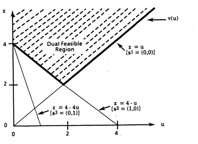
Figure 5.2 illustrates this procedure and serves as motivation for our subsequent analysis. In the figure, we have plotted the three constraints from the dual version (5.3.10) of the subproblem. Note that as a function of u, the minimum objective function value v(u) to the problem is the upper

envelope of the three lines in the figure. At u - 0, the lines z - 4-u and z - 4-4u both pass through this lower envelope. Equivalently, the extreme points 2 - (1,0) and 3 - (0,1) of the dual feasible region S both

solve the dual problem. Note, however, that as we increase u from u - 0, the line z = 4-u lies above the line z - 4-4u. It, therefore, provides a better approximation to the dual objective function v(u). To identify this preferred line, we can conceptually pivot about the solution point (z,u) (4,0),

choosing the line through this point that lies most to the "northeast". Note

4

0

OP / l .,// . V(U)

DualFeasible

-~

Region

-

-3

][st

=

(0,0)]

/\ U

z=4-u

z = 4-4u

<

[s2 = (1,0)]

[S3 (0,1)-- I1

Figure 5.2 Subproblem (Dual) Feasible Region

_, _

I I

that to discover this line, we need to find which of the two lines through the pivot point (z,u) is higher for any value of u > 0.

Before extending this observation to arbitrary minimax problems, we formalize some definitions.

We say that the cut (or constraint) z > f(s) + ug(s1 )

in the minimax problem (5.3.7) dominates or is stronger than the cut

z > f(s) + g(s)

if

f( 1) + ug(sl) > f(s) + g(s)

for all uU with a strict inequality for at least one point uJU. We call a cut pareto-optimal if no cut dominates it. Since a cut is determined by the vector seS, we shall also say that s dominates (is stronger) than if the associated cut is stronger, and we say that is pareto-optimal if the corresponding cut is pareto-optimal.

In the previous example, we showed how to generate a pareto-optimal cut by solving an auxiliary problem defined by any point u > 0. Note that any such point is an interior point of the set {u: u > O}. This set,

in turn, is the convex hull of the set U {u: u > 0 and integer}.

The following theorem shows that this observation generalizes to any minimax problem of the form (5.3.7). Again, we consider the convex hull of U, denoted U,

but now we will be more delicate and consider the relative interior (or core)t of UC , denoted ri(UC), instead of its interior.

t The relative interior of a set is the interior relative to the smallest affine space that contains it. For example, the relative interior of a disk in 3-space (which has no interior) is the interior of the disk when viewed as a circle in 2-space.

- 26

-The result will always be applicable since the relative interior of the convex set U is always nonempty. For notation, let us call any point u

contained in the relative interior of U c, a core point of U.

Theorem 5.1: Let u be a core point of U, that is, u c ri(U ), and let S(u) denote the set of optimal solutions to the optimization problem

maximize {f(s) + tg(s)}. (5.3.11)

sES

Also, let u be any point in U and suppose that a solves the

problem-maximize f(s) + uOg(s)}. (5.3.12)

soS(u) Then s is pareto-optimal.

Proof: Suppose to the contrary that s° is not pareto-optimal; that is, there is a s that dominates . We first note that the inequalities

f(i) + ug(i) > f(s°) + ug(s) for all ucU, (5.3.13) imply that

f(i) + ug(i) > f(s°) + ug(8s) for all UCUc. (5.3.14) To establish the last inequality, recall that any point cUC can be expressed

as a convex combination of a finite number of points in U, that is,

u -

{AUU: uU} - 1

Uu

where > 0 for all uU, at most a finite number of the Xu are positive, and

I

X - 1. Therefore, (5.3.14) with u - u can be obtained from (5.3.13) by uCU

multiplying the u inequality by X and adding these weighted inequalities. U

Also, note from the inequality (5.3.13) with u - u that must be an optimal solution to the optimization problem (5.3.11) when utr, that is, i6E(u). But

then, (5.3.12) and (5.3.13) imply that f(s) +

u

_{g(s1 - f(so) + u g(O). (5.3.15)} O Since dominates 8 , f(B) + ug(B) > f(s°_{) + ug(s}°₎ (5.3.16) for at least one point uU. Also, since u ri(U ) for some scalar > 1

u 8 uO + (1 - )

belongs to U. _{Multiplying equation (5.3.15) by , multiplying inequality} (5.3.16) by (1 - _{), which is negative and reverses the inequality, and} adding gives

f(i) + ug(1) < f(s°_{) + ug(s}0_).

But this inequality contradicts (5.3.14), showing that our supposition that s0 is not pareto-optimal is untenable.

We should note that varying the core point u might conceivably

generate different pareto-optimal cuts. Also, any implementation of Benders' algorithm has the option of generating pareto-optimal cuts at every iteration,

or possibly, of generating these cuts only periodically. The tradeoff will depend upon the computational burden of solving problem (5.3.12) as compared

to the number of iterations that it saves.

In many instances, it is easy to specify a core point u for implementing the pareto-optimal cut algorithm. If, for example,

U _{{ueRk:u > 0 and integer}}

then any point u > 0 will suffice; if

U = {ueRk: uj - 0 or 1 for j 1,2,...,k}

then any vector u with 0 > u > 1 for j - 1,2,...,k suffices; and if k

U - {uRk : z uj p, u > and integer}

J'1l