HAL Id: inria-00274399
https://hal.inria.fr/inria-00274399
Submitted on 18 Apr 2008
HAL is a multi-disciplinary open access
archive for the deposit and dissemination of
sci-entific research documents, whether they are
pub-lished or not. The documents may come from
teaching and research institutions in France or
L’archive ouverte pluridisciplinaire HAL, est
destinée au dépôt et à la diffusion de documents
scientifiques de niveau recherche, publiés ou non,
émanant des établissements d’enseignement et de
recherche français ou étrangers, des laboratoires
Conformance Testing based on UML State Machines:
Automated Test Case Generation, Execution and
Evaluation
Dirk Seifert
To cite this version:
Dirk Seifert. Conformance Testing based on UML State Machines: Automated Test Case Generation,
Execution and Evaluation. [Research Report] 2008. �inria-00274399�
Conformance Testing based on UML State Machines
Automated Test Case Generation, Execution and Evaluation
Dirk Seifert
LORIA— Universit´e Nancy 2, Campus scientifique, BP 239 54506 Vandœuvre l`es Nancy cedex, France
Abstract. We describe a comprehensive approach for conformance testing of reactive systems. Based on a formal specification, namely UML state machines, we automatically generate test cases and use them to test the input-output con-formance of a system under test. The test cases include not only the stimuli to trigger the system under test, they also include the test oracles to automatically evaluate the test execution. In contrast to Harel Statecharts, state machines be-have asynchronously, which makes automatic test case generation a particular challenge. As a prerequisite we have completely formalized a substantial subset of UML state machines that includes complex structured data. The TEAGERtool suite implements our test approach and proves its applicability.
1
Introduction and Related Work
The impact of embedded systems in our everyday life is steadily growing. They are present not only in very specific contexts, but also in nearly every electrical device we use. In general, embedded systems comprise of hardware and software components in-teracting with a specialized technical environment via sensors and actors. The main reason for their success is the combination of specific or high-performance hardware with the flexibility of software. The software is responsible for controlling the hardware and software components and for calculating reactions as responses to received events. Erroneous systems annoy the costumers and are a high commercial risk in mass cus-tomization. Moreover, size and complexity of nowadays systems demand for improved and automated processes: for development as well as for quality assurance.
In a model-based development approach, models of the system which have to be built, guide and control the development process. There are various types of models dif-fering in the level of abstractions or in their intended use. In the first steps, the models are used to analyze the problem domain and to ease the information exchange among developers. Later on, they form the basis to design and implement the system, serve as documentation, and are also used for quality assurance purposes. For example, the Unified Modeling Language (UML) comprises thirteen diagram types to specify the structure and the behavior of a system or a system component [1]. The included state machines are used to either describe the discrete reactive behavior (behavioral state ma-chines) or to describe the usage protocol (protocol state mama-chines). In our approach we use the behavioral state machines to specify the states a system can take and actions
it can execute during its lifetime in response to internal and external events. The dis-crete reactive character of state machines and the possibility to completely specify the behavior of a system make state machines appropriate to model reactive systems. They also allow to automatically generate test cases that include test oracles. Testing means executing a system under test (SUT) with selected but real data to evaluate its confor-mance, whereat conformance is evaluated on the basis of the observations made on the system under test. It aims in falsification, that means to show inconsistencies between the specification and the SUT. It benefits from the fact that the actual system is brought to execution, and thus, the interaction of the real hardware and software can be evalu-ated. It also benefits from the fact that it is applicable at different levels of abstraction and at different stages of the development.
The contribution of our work is twofold: first, we formalized a substantial subset of UML state machines that includes the manipulation of complex structured data. Second, we present a conformance test approach based on UML state machines that allows automatic generation, execution and evaluation of test cases on the level of unit testing. To our knowledge there is no formalization related to the latest UML standard [1] that precisely formalizes data aspects. We focus on the reactive behavior and skip real time aspects in this paper (in short: we allow to manually specify lower and upper timeout limits for every event). Considering real time behavior is still a challenge for automated processes. It is one of our prospects for future work.
Our formalization of UML state machines is influenced by several works (e.g., [2– 4]). Most approaches focus on model checking and the chosen representation is not al-ways appropriate for automated test case generation. Moreover, there have been major changes in UML 2 that require a revision of previous works. We present an operational semantics that is complete with respect to the considered subset and includes all nec-essary definitions. Moreover, it is the first formalization which includes all definitions related to complex structured data. De Nicola and Hennessy [5] introduce a formal the-ory of testing on which (later on) Brinksma [6] and Tretmans [7] build approaches to derive test cases. For basic work on testing based on transition systems and (extended) finite state machines we refer to the surveys [8–10]. A lot proposals only deal with de-terministic systems and require that the model must be strongly connected [11–13], or assume the testing process to communicate synchronously with the system under test [6, 10]. More recent research allow some of these requirements to be relaxed (see e.g. [14–16]) but most refer to older UML standards, consider different subsets, or do not consider complex structured data. Moreover, we allow nondeterminism in the specifi-cation as well as in the SUT, and asynchronous communispecifi-cation between the SUT and its environment. A further difficulty in using transition or finite state machines based techniques is that transitions in state machines are labeled with input-output pairs as-sociated to a single transition. The underlying semantic model builds on the steps of the whole state machine. Those comprise the execution of several transitions including changing the current configuration and executing actions such as those that generate output events. In such a step the atomicity of input processing and output generation is preserved. Mapping the semantics to transition systems or input/output automata to apply classical techniques would require to introduce intermediate states and transi-tions. On the one hand this would break the correspondence of a state machine step
and a semantic step, and on the other hand such a multi-step approach unnecessarily complicates the formalization and use of state machines.
Latella et al. [15, 17, 18] follow (as we do) a ”semantics-first” approach in which a sound basic kernel of the notation is considered and extended, only if the main features are investigated. In contrast to our work they do not consider complex structured data (i.e., interpret a state machines data space or event parameters). They also refer to an older UML standard and do not consider different transition orders, which become rel-evant if data are regarded. Offutt et al. [19, 16] present techniques to generate test cases from UML state diagrams on class-level testing. In contrast to our work, they have a data-centric view and focus on change events and boolean variables. The generated test suites are related to full-predicate coverage. Moreover, it is not clear how far the ap-plied semantics follows the UML standard. The work around the AutoFocus tool [20] is interesting but they use proprietary notation which does not include all aspects of UML state machines and a formal, but synchronous, semantics. Another mentionable industrial approach are the AGEDIS tools [21], but the used semantics is not completely clear. Spec Explorer developed at Microsoft Research ([22] and related publications) is an industrial approach that uses finite state machines as the underlying model for au-tomated testing. They also test against nondeterministic systems and address problems of data instantiation. The general principle to explore the specifications state space is comparable to our approach. In contrast, the focus is on (synchronous) method calls.
In Sec. 2 we introduce the syntax and semantics of state machines we need in this paper by means of an example. In Sec. 3 we present our test approach to automatically generate test cases out of a state machine specification. We describe the underlying theory, the test case generation algorithms, how approximation techniques are used to increase the efficiency and how the test case generation and execution can be controlled and evaluated. In Sec. 4 we present our TEAGER tool suite and discuss experimental results. In Sec. 5 we conclude our work and give an outlook to ongoing research.
2
State Machines
UML state machines [1] are an object-oriented extension of the classical Harel State-charts [23]. We use them to describe the sequence of states a system or system compo-nent can take and the actions it executes when changing these states. State machines are mathematical models with a graphical representation: the nodes depict simple or com-posed states of the system and the labeled edges depict transitions between these states. Composite states are used to hierarchically and orthogonally structure the model, thus reducing its graphical complexity. Labels express conditions under which transitions can be taken and the actions that will be executed when the transitions are taken. Events are used as triggers to activate transitions and can be parameterized to exchange data. Optional, every state machine has a data space that can be read and manipulated by the state machine during execution. More precisely, it is possible to read data values to describe specific conditions when a transition can be taken or to manipulate data values and exchange information within actions. A transition comprises a source state, a trigger event, an optional guard, an optional effect (which consists of a sequence of actions), and a target state. A guard describes a fine-grained condition (with reference to the
sys-EmptyCD Full CD boolean inCDFull = false; boolean inTapeFull = false; integer trackCount;
power power Audio Player Off
On CD Mode CD Player next back next next back back back next next back P2 P3 P4 Tuner Mode
src [ in("Tape Full") ] / tape_plays src [ not in("CD Full") ] / tuner_plays
src [ in("Tape Full") ] / tape_plays src [ in ("CD Full") ] / cd_plays src [ in("CD Full") ]
/ cd_plays
/ tuner_plays src [ not in("Tape Full") ] cd_eject
tape_eject [ in("CD Full") ] / cd_plays tape_eject [ not in("CD Full") ] / tuner_plays
Tape Mode Spooling Backward Forward Spooling PlayingTape back back next next
cd_insert / inCDFull = true; trackCount = cd_insert.1
cd_eject / inCDFull = false;
EmptyTape
tape_insert / inTapeFull = true; Tape Player
tape_eject / in TapeFull = false; Car Audio System
CD Playing play Track Next play Former Track Full Tape P1
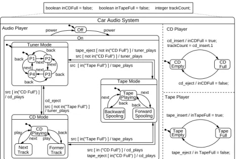
Fig. 1. State machine specification for the Car Audio System.
tem’s state) that must evaluate to true to enable the transition. Hence, the activation of the source state, the trigger event and the fulfilled guard condition constitute the neces-sary constraint to fire a transition. An action can either be a statement manipulating the data space or the generation of new events. The action sequence and the subsequently active target state constitute the overall effect of the transition. In opposite to the clas-sical Statecharts, the event processing takes place in a so-called run-to-completion step [1]. This asynchronous event processing demands the processing of the previous event to be completely finished before the next event can be processed. In the following we briefly describe state machines by means of an example. Afterwards we discuss se-mantic issues which pose a challenge for automated test case generation. A complete and detailed description as well as a precise definition of the semantics (including the integration of complex data) can be found in [24, 25].
2.1 Example
We use a state machine model specifying the behavior of a simple sound device in a car to demonstrate the state machine notation. The requirements for such sound device could be as follows: It should be possible to turn the Car Audio System on and off.
When turned on, it should play one of three different audio sources, namely radio, tape or compact disc, respecting the presence of a tape or a compact disc. It should be possible to change between available sources. Furthermore, it should be possible to switch between four radio stations, to spool a tape backward or forward, or to select the previous or the next track of a compact disc.
We introduce the following events to model the required behavior: power, src (to switch between the different sources), next, back and play. We also intro-duce events signaling the insertion and the ejection of a tape or a compact disc as
well as events to signal system reactions. Furthermore, we use data variables to store detailed information about the current state. For example, we use an integer variable trackCountto store the number of titles of an inserted compact disc. Figure 1 shows a state machine model of the sound device including the related data space.
At the highest level of abstraction the model consists of an orthogonal state com-prising three regions. The two regions CD Player and Tape Player model the information if a tape or a compact disc is inserted into the system or not. The more com-plex region Audio Player models the control of the system. The region is refined by two states: Off and On. Initially the system is assumed to be switched off, expressed by the small arrow leaving a bullet and ending at the Off state. When the event power is processed the system is switched on and starts to play the radio (again expressed by a small arrow). The composite state On is refined into states modeling the three signal sources. The transitions between these states describe the changes between the sources as reaction to an event src. For example, when the system is in Tuner Mode and a tape and a compact disc are inserted into the system (i. e. both in-predicates are true) and the event src is processed, the system can either switch to the tape mode or switch to the compact disc mode because both transitions are enabled and can fire. All three substates of Audio Player are further refined to describe the particular behavior in reaction to the events next, back and play in each state.
2.2 State Machine Semantics
The semantics of UML state machines is adapted from the STATEMATEsemantics [26] to fit into the object-oriented paradigm. As described above a state machine can be refined by simple composite and orthogonal states. Simple composite states contain exactly one region and orthogonal states contain at least two regions. In every region only one substate can be active at a time. The state which is entered by default when a region is entered is marked by an arrow emanating from a filled circle. The hierarchical ordering of states forms a tree structure with a region as the root node, simple states at the leave nodes and in between (alternating) composite states and regions.
Due to orthogonal regions a state machine can have several active states at a time. We call the set of all active states configuration. For the same reason it is possible that more than one transition can fire at a time — one in every active orthogonal region. We call the set of all jointly firing transitions firing transition set (FTS). Due to the hier-archical structure it can happen that two transitions are enabled for firing on different hierarchy levels of a state. Taking both would lead to a configuration which is not well-formed. A similar situation arises if a transition leaves an orthogonal region. In this case the transition cannot fire together with an enabled transition in another orthogonal region. In both cases the transitions are said to be in conflict with each other. Conflicts are identified if two transitions leave identical states in the state hierarchy. The UML describes a two-step process to resolve conflicts. In the first step a priority scheme is used. A transitions emanating from a state deeper in the state hierarchy has priority over the other transition. Thus the more refined transition is taken. This differs from classi-cal Statecharts, but it reflects the object-oriented inheritance behavior. However, not all conflicts can be resolved using this priority scheme. In the second step only transitions are selected which are not in conflict to each other allowing for maximal progress of
the system. A so-called transition selection algorithm selects all maximal sets Tk⊆ T
of enabled transitions fulfilling the following requirements:
∀ t : Tk• enabled (t, c, e, d) (1)
∀ t1, t2: Tk| t16= t2• t1k t2 (2)
∄ t′: T\ T
k| enabled (t′, c, e, d) • ∀ t : Tk• t k t′∨ t′≺ t (3)
First, all transition in the set must be enabled regarding the current configuration, the trigger event and the current data assignments. Second, all transitions in the set are mutually conflict free (expressed by thek operator). Third, there is no enabled transi-tion outside the set which is conflict free with all transitransi-tions in the set or with higher priority than a transition inside the set. Thus, transitions with the highest priority are taken and maximal sets are chosen. Result is a set of firing transition sets (FTSs). It is important to mention that for execution one FTS is arbitrarily chosen, and that the order in which the transitions in this set are fired is arbitrarily chosen, too. In consequence, all set choices and transition permutations form the set of all possible semantic steps of the state machine at a time. This is important if we want to compute the possible correct behavior for an input sequence to evaluate the test execution. In opposite to classical Statecharts, the event processing takes place in a so-called run-to-completion step. This asynchronous event processing demands the processing of the previous event to be completely finished before the next event can be processed. Therefore it is nec-essary to buffer received events in an event store. Consequently, the occurrence of an event and its processing are asynchronous (i.e., take place at different times). It follows that a possible (observable) reaction of the system also takes place asynchronously.
The semantic model of state machines builds on the semantic steps a state machine can execute during its lifetime. Such a step moves the state machine from one semantic state to another semantic state while receiving events from and emitting events to the environment. A semantic state (called a status) comprises three components, namely a configuration (a set of active states), an event store, and the variable assignments. We depict the components of a status in double square brackets[[c, q, d ]] and a semantic step [[c, q, d ]]−−−→ [[cin, out ′, q′, d′]]. Note that the chosen set of firing transitions and the execu-tion order of these transiexecu-tions can be identified (if necessary) from this representaexecu-tion. Assuming a state machine to be input enabled (cf. the next section) a semantic step can be described as follows: q=<> q′= ⊕(q, Ein) [[c, q, d ]] Ein,hi −−→ [[c, q′, d ]] (4) q∈ ran ⊕ (q′′, e) = ⊖(q) c′= (c \S∀ t:Tkexits(t)) ∪S∀ t:Tkenters(t)
Aseq∈ perm({t : Tk• effect (label (t)(e))})
(d′, Egen) = performAll(a/ Aseq)(d)
(Eint= Egen↾ ESM) ∧ (Eout= Egen↾ Eenv) q′= (q′′⊕ Eint) ⊕ Ein
[[c, q, d ]] Ein,Eout
−−−−→ [[c′, q′, d′]]
We have to distinguish two situations. First, the situation when the event store does not contain any event (4). During the step, only the events received from the envi-ronment (Ein) are added to the event store (⊕(q, Ein)). The active configuration and
the data assignments are left unchanged. Second, the situation when the event store contains events for processing (5). During the step, the trigger event will be selected from the event store (⊖(q)). The next configuration c′ results from leaving all states
the transitions exit, and entering all states the transitions enter. Next, an execution order for the FTS is chosen (perm), and the effect of this transition sequence is calculated (performAll). The effect includes the new data assignments (d′) and the sequence of newly generated events (Egen). Finally, this event sequence is processed. The generated
internal events (Eint) and the events received from the environment (Ein) are added to
the event store. The remaining external events (Eout) are sent to the environment. Now
we can describe the execution of a state machine based on this definitions as a concate-nation of semantic steps. We call such a sequence of semantic steps a computation.
[[c1, q1, d1]]
in1, out1
−−−−→ [[c2, q2, d2]]
in2, out2
−−−−→ . . .−−−−−−−→ [[cinn−1, outn−1 n, qn, dn]]
We use this execution model to define our test approach. Only a precise and clearly interpretable mathematical model as we presented here offers the basis for automated processes. Our complete state machine semantics can be found in [24, 25].
3
Test Case Generation
In the UML standard and in our semantics, too, not all semantic details are completely determined. These open issues are called semantic variation points. They prevent un-necessary restrictions in the semantics and allow some degrees of freedom for the im-plementation of the semantics. The user has to instantiate them before working with the semantics. Unfortunately, many problems with the UML semantics arise from semantic variation points. On the one hand some of them are not obvious in the standard and on the other hand decisions taken are often not propagated to the public. Concerning our test approach the most interesting semantics variation points are: the nature of the event store, events not enabling any transition, the selection policy of possible firing transition sets, and the execution order of the transitions in a chosen set.
We instantiate the two first semantic variation points and do not instantiate the latter two, thus the test approach works correctly for different implementations of a state machine specification. Precisely, we neither want to restrict how to choose a possible set of firing transitions (if there is more than one) nor do we want to restrict the order these transitions will be executed. This is different for the event store. In order to be able to calculate the possible correct behavior allowed by the state machine specification, we need to know the nature of the event store, or with other words, we have to decide for a specific nature. In most practical contexts a FIFO queue is used to store events for further processing. Hence we assume an unbounded reliable FIFO queue as event store. Second, we assume that events that do not enable a transition when they are processed are deleted and the next event from the event store will be processed. This implies that the state machines do not block. Technically they are called input enabled. In summary,
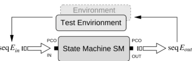
PCO IN PCO OUT State Machine SM Test Envirionment Environment seq Eout seq Ein
Fig. 2. Abstract test assembly for reactive systems.
an event queue is introduced into the semantic model of state machines, non-enabling events from the queue will be omitted, and we need to respect different firing transition set selection and execution strategies in our test approach.
3.1 Conformance Relation for State Machines
As mentioned in the introduction, an embedded system usually comprises of hardware and software components. Hence, we treat the SUT as a black box to reflect this cir-cumstance. We only require the SUT to have so-called points of control and
observa-tions. With these it is possible to control and observe the SUT. (i.e., to send inputs and
to observe the outputs of the SUT). Figure 2 shows this abstract test assembly. As a consequence only the inputs to the SUT and the outputs of the SUT are visible in the environment and thus for the tester. This particularly implies that the event queue is not visible from the outside. To generate test cases and especially the test oracles we need to restrict the test generation to the observable parts of a SUT, but must respect internal details, which influence the possible behavior. Consequently, we need to extract the ob-servable parts of the computations we defined for the semantic model of state machines. These are the events received from the environment and the generated events sent to the environment. Corresponding to the computation defined above we yield an observable
computationby extracting and concatenating these events:
in1a out1a ... a inn−1a outn−1 (6)
We assumed the event store to be a queue so that received events will be stored one after another in sequence. Furthermore, we assume that transitions and actions on tran-sitions are executed in sequence. Hence, generated events are also stored in sequence. The set of all observable computations form our observable execution model of state machines and the basis for the test case generation.
A prerequisite to automatically evaluate whether a SUT conforms to its specification is a precise definition of conformance. De Nicola and Hennessy studied various possi-ble characterizations of conformance [5, 27]. Brinksma and Tretmans studied various implementation relations for synchronous transition systems [6, 7]. In general, relevant implementation relations are based on the same idea of an external observer. Here, an implementation I conforms to its specification S, if and only if, all observations obs any external observer o : O can make on the implementation, can be related to the observa-tions this observer can make on the specification:
To get an applicable relation you need to define the type of observers (O), which observations these observers can make (obs), and how to relate these observations (⊑). We use sequences of inputs to the SUT as observers. The observations these observers can make are the resulting outputs (i.e., the generated events). The relation we use to compare observations of the system under test with the observations of the specification is set inclusion (⊆). We argue that a system under test conforms to its specification, if and only if, the output sequences for all possible input sequences are included in the set of all output sequences of the specification for the same input sequence (8). Following Tretmans [7] we restrict the set of possible inputs to that of the specification (seq ES). The set of outputs we calculate from the set of observable computations of a speci-fication (9). Precisely, the set of all observations out(S, σ ) for S with input sequence σ results from all observable computations of S (otraces(S)) for which σ denotes the input sequence (σ= δ ↾ ES) and δ ↾ Eenvdenotes the resulting output sequence.
I≤outS⇔ ∀ σ : seq ES• out(I, σ ) ⊆ out(S, σ ) (8) out(S, σ ) == {δ : otraces(S) | σ = δ ↾ Ein• δ ↾ Eout} (9) Now we have a precise meaning of conformance and a guideline how to compute test cases and test oracles: based on the specification we need to calculate the traces of the state machine for all possible inputs and extract the possible correct observations. For testing we need to stimulate the SUT with the particular inputs, observe the outputs and compare them to the pre-calculated possible correct observations. That means to check for their existence. Obviously a problem arrises when thinking about practical testing — the set of inputs is usually infinitely large or at least pretty huge.
3.2 Selecting Inputs for Test Case Generation
When testing in practice we are only interested in relevant and interesting test cases to advantage the quality assurance process, and to use time and computation power at an optimum. Therefore, we generate test cases for pre-selected input sequence. This two-step process clearly separates the input selection problem from the test case generation problem. Hence it is possible to use different selection strategies with the same genera-tion process and it allows to adapt the input selecgenera-tion process to different test purposes or to different project stages.
In the TEAGER tool suite we implemented several input selection strategies. The strategies range from using given fixed input sequences to using specific models de-scribing the environment. The former allows special value testing and is used for very specific test purposes like the coverage of a certain path or state. The latter allows to model varied behavior of an environment based on probabilities. The most general one is an environment in which all inputs can happen at any time with the same probability (uniform distribution). In a more specific environment different probabilities are as-signed to the inputs (a prior distribution). Thus the occurrence of specific inputs can be influenced. We also use a variant of this strategy where we adapt the probabilities once an input is chosen (dependant distribution). For every input a weight is assigned and decremented if the input is selected. If all weights are equal to zero the initial assign-ments will be used. With this strategy we ensure that eventually every event is chosen.
The most expressive way to describe the environment is to model it with probabilistic state machines. Using state machines allows to model dependencies among inputs in a sequence. It also allows to completely reassign input probabilities depending on the assumed state of the system under test. For example, the probability of dialing a num-ber before lifting the receiver of a telephone is certainly different from the probability of dialing after lifting the receiver. In summary, we use different complex strategies to describe assumed environments to select relevant and interesting inputs. For a detailed description of our input selection strategies we refer to [28].
3.3 Test Case Generation Algorithm
During test case generation we consider a finite set of finite sequences of inputs and calculate all possible correct observations for these inputs. We use these observations to automatically evaluate the test execution process. Considering complex data during the test case generation process is not scope of this paper and we skip the corresponding details here. The problem which specific data to choose is part of ongoing research. In the current approach data are chosen randomly during the test case generation.
To calculate the possible correct observations we stepwise explore the state ma-chine’s state space for the given input. The challenge is to correctly consider all seman-tic subtleties. We do this in a two step algorithm. First, we initialize the state machine with its initial status (i.e., with its initial configuration, an empty queue and an initial data assignment). We insert the first input event to the event queue and apply a semantic step to this configuration. This includes that we calculate all possible FTSs. For every FTS and every possible execution order of the transitions inside these sets we calculate the resulting status. It is important to note that we calculate a fix-point for this set. That means, that no new status can be reached from any calculated status. Thus we yield a set of all reachable status including all intermediate status for the first event. To store the intermediate status is important for handling possible interleavings of input and inter-nally generated events. Second, we insert the next event to every reachable status in the previously calculated set. Thus we respect possible interleavings of events in the event queue. Then we again calculate all reachable status for this input and proceed in the same way for the remaining inputs. Consequently, we calculate the graph of all execu-tion paths including the reachable status. Only this stepwise calculaexecu-tion of all reachable status ensures that all possible execution paths for the given input sequence are cal-culated. This includes all non-determinism in the specification (modeled and arising from the semantic model of state machines) and effects from processing events asyn-chronously. Figure 3 visualize the principle of the calculation of an execution graph for the abstract input sequence [a,b,c]. The red parts show the newly calculated parts in the subsequent step. For example we can see that by processing the queue [a,b] we reach different status than by processing both events separately.
In the following we illustrate the key point of the algorithm by means of an short abstract example. Let us assume that an internal event i is generated when processing an event a. Let us further assume that processing an i will produce an internal event j. For the next test case we want to process the input sequence a·b. During test execution we have to trigger the SUT first with a and then with b with an (currently) undefined time gap between the events. The challenge is that we cannot predict the actual queue
a a 01 b b b b b a c c c c c c c c b a 0 1
Fig. 3. Stepwise state space exploration for the input sequence [a,b,c].
of the SUT during test case generation. Consequently we do not know how event b will interleave with the internally generated events i and j. For this reason we first insert a into the queue and calculate the three reachable status: [i],[j],[]. The first queue results from just processing a. The second results from processing a and then i and the third results from processing a, then i and then j. By inserting b into all reached queues we prepare for respecting all possible interleavings. The resulting queues are [i,b], [j,b], [b]and during the next step [b,j] which properly respects one possible interleaving. Event b will also be inserted to the queue [a] resulting in queue [a,b]. This reflects the situation that we triggered both inputs before the system under test processed the first one. Figure 3 visualize this situation in the second graph.
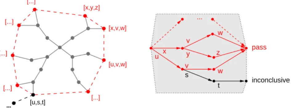
After processing all events from the input sequence we can identify among the set of all reached status those status which are finally reached. These status (located at the hull of the execution graph) are quiescent. That means that their event queue is empty and thus they cannot proceed without a new input from the environment. Figure 4 shows at the right side an execution graph with the reached status at the hull. We extract from these the observations that would be emitted (i.e., the events the state machine sends to the environment) when executing this particular path. The extracted observation se-quences comprise all possible correct observations we can make when triggering the system under test with the input sequence. Now the idea is to treat all observations as the alphabet of a language and the calculated observation sequences as accepted words of these language. Accepted observation sequences cause the test execution to pass. All other sequences cause the test execution to fail. Now we just need to build an acceptor for the calculated observation sequence and use them as the test oracle.
Finally, we need to overcome one open problem which can arise when calculating the execution graph. We previously mentioned that we determine for an input sequence the fix-point for the reachable status. Due to the fact that state machines can generate (internal) events and produce internal infinite loops the calculation of these fix-points does not terminate in any case (we also subsume the problem that the time to calculate the fix-point is unacceptable high). To overcome this problem we limit the number of steps needed to calculate all subsequent status to an upper bound. Technically, every reached status has got a counter for the number of steps necessary to reach this status. If a counter reaches the specified upper bound we mark this status and abort further processing of this status. Figure 4 shows this in the lower left corner.
As a consequence we calculate two types of observation sequences. One which could be calculated within the given bound, and one which could not. The latter type
... [...] [u,s,t] [...] [...] [...] [...] [x,y,z] [x,v,w] [u,v,w] inconclusive ... pass w w t s v u x y v z
Fig. 4. Execution graph and the resulting acceptance graph with an inconclusive verdict. could be interpreted as follows: all observations made so far are correct, but not all observations could be calculated. For the test execution and evaluation this means that after processing all calculated observations, we have no further observations to which we can compare the remaining outputs of the SUT. We can neither say that further ob-servations are correct nor can we say that they are not. We can only stop testing the SUT with this input sequence and give an inconclusive test verdict. This verdict says that all observations so far are correct but that we stopped further processing the cur-rent execution path. It would also be possible to decide for a pass or a fail verdict. But introducing a third verdict allows a finer distinction of differently caused test execution results. Hence, we distinguish two sets of possible observation sequences and the ac-ceptance graphwe build out of these sets comprises two accepting nodes. One for all observation sequences which could completely be generated and one for all observation sequences which were bounded. The acceptor itself is a deterministic finite automaton accepting both sets of observation sequences. A test case execution finishing in one of these nodes results in a pass or an inconclusive verdict. All observations not covered by the acceptance graph result in a fail verdict. On the right side of Fig. 4 you can see an acceptance graph for the execution graph on the left side.
A test case comprises the input sequence to stimulate the system under test and an acceptance graph to automatically evaluate the execution of this test case. The length of a test case and the number of test cases can be influenced by the selection policy of input sequences as explained above. The generated test suite is sound. That means that no correct systems under test will be rejected due to a test case. Instead, the test verdict fail will only be assigned if the observation of the system under test cannot be explained by the possible correct observations of the specification (see the conformance relation for state machines). This is true because we calculate all possible execution paths to generate the sets of possible correct observations. With unlimited computation power and time the presented algorithm is able to compute a complete test suite, which is capable to exactly differentiate between correct and incorrect implementations.
Algorithm 1 shows the control structure of the test case generation algorithm. The loop will be executed as often as inputs should be sent to the system under test in the test case. The inner while-loop controls the fix-point calculation of reachable status. While there are newly generated status the simulation step is successively repeated to calculate all reachable status. If there are no newly generated status the algorithm
input : state machine:sm
output: an acceptance graph
sm.configuration← initial configuration
result← initial simulation node
inconclusives← ∅
while|trigger| <input lengthdo
trigger← generate a new trigger
store← ∅
forallnode∈resultdo
node.queue⊕trigger store∪ {node}
steps← 0
whileresult6= ∅ ∧steps<limitdo
temp← simulationStep(result)
steps←steps+ 1,result← ∅
forallnode∈tempdo ifsteps=limitthen
inconclusives∪ {node} else
store∪ {node}
result∪ {node}
result←store;
generateAcceptanceGraph(result,inconclusives)
Algorithm 1: Test case generation: control structure.
proceeds with the next input event. The results of the loop are a set of all completely calculated observation sequences and a set of all incompletely calculated observation sequences. Out of these sets an acceptance graph will be calculated.
Algorithm 2 shows the calculation of the successive status for the calculated status in the previous step. First, the state machine is initialized with the configuration from the status and the next trigger event is selected from the corresponding event queue. Then, all possible FTSs and all possible transition execution orders are executed to estimate the resulting status and the generated events. This includes: saving reached configuration, adding internal events to the input queue, and saving generated events which should be sent to the environment. The latter events are the possible correct observations which we use to build the acceptance graphs. Both the successive status and the generated events will be stored in a new simulation node. The set of all new simulation nodes will be returned as the result of the simulationStep.
The presented algorithm has exponential complexity. This complexity arises from the branch factor introduced by the different sets of firing transitions, the different pos-sible execution orders of transitions, and the necessity to consider pospos-sible interleavings in the event queue (asynchronous event processing and non-observable event store). The effort to calculate a test case grows with the length of an input sequence ˜x and indirectly by the number of internally generated events (expressed as a functional relation: f(˜x)). The branch factor is bounded by the finite number of transitions and the finite number
input : set of simulation nodes:input
output: set of new generated simulation nodes:result
result← ∅
forallnode∈inputdo ifnode.queue6= <> then
sm.configuration←node.configuration
event←node.dequeue
forall Tk:sm.getFTS(event)do
permutations← permute(Tk)
forallfiring transitions:permutationsdo
effects← [ ]
forallt:firing transitionsdo
effects← fire(t)
temp←node
temp.configuration←sm.configuration foralleffect:effectsdo
forallev:effectdo ifev∈ E/ SMthen temp.observation⊕ev else temp.queue⊕ev; result∪ {temp}
sm.configuration←node.configuration returnresult
Algorithm 2: Test Case Generation: Simulation Step.
of events (c). Thus we can approximate the effort A to generate a test case for a given input sequence of length x as follows:
A(x) ∼ ec· (x + f (˜x)) (10)
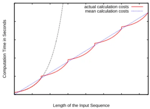
This exponential effort is visualized in the left diagram in Figure 5 by the gray doubly dotted graph. Due to the character of state machines this exponential effort can-not be avoided when pre-calculating test oracles. To weaken this problem we are also working on strategies to split input sequences and to combine test cases, respectively.
3.4 Combining Test Sequences
When testing non-terminating reactive systems it is also interesting to execute longer input sequences. To reduce non-determinism in the specification is not possible with-out any further knowledge abwith-out the system under test. Thus we concentrate on the asynchronous event processing. The lion’s share of the calculation effort results from respecting all interleavings of the input sequence with internal generated events. We can argue that it is not necessary to consider all of these interleavings. For example, in practice it is the case that the system under test immediately starts to process the first
Computation Time in Seconds
Length of the Input Sequence actual calculation costs
mean calculation costs
Fig. 5. Linearization of the exponential Complexity.
received input. It usually does not wait until ”ten” events are received from the environ-ment. With the distance of two events in the input queue the probability decreases that an internally generated event (as a consequence of processing the first event) interleaves with the second one.
Based on this idea we developed various strategies to reduce the calculation effort. To demonstrate the core idea we implemented a strategy where we introduce so called
observation points. Observation points are points in time where we give the system
un-der test enough time to calculate its reaction. Related to our semantic model of state machines the system under test reaches a status in which the event queue is empty. Hence, no more reaction can be produced for the given inputs. This is true for all status at the hull of the execution graph from the previous section. Continuing after such an observation point now means: to enqueue the next input to all (non-inconclusive) status on the hull of the previously calculated execution graph (note that for these status the event queue is empty). We also reset the collected possible observations and calculate the corresponding acceptance graph. This is possible because we assumed that the sys-tem under test has completely calculated its reactions. Now we proceed to calculate the possible correct observation sequences for the complete next input sequence. An im-provement of this strategy is to collect possible correct observations for more than one observation point and then generate one acceptance graph for all input sequences.
The reduction in the computation effort results from the fact that we do not consider possible interleavings resulting from events in the previous input sequence with events in the next input sequence. The left diagram in Figure 5 visualizes this procedure. We repeatedly calculate only the first part of the exponential curve. The overall calculation effort follows from adding the efforts needed to calculate the observations for the indi-vidual input sequences (the red graph). The average effort has a linear gradient depicted by the blue dotted graph. Compared to the effort for processing one input sequence with the length of the sum of all sub-sequences this is an enormous reduction in the calcu-lation effort. The effort for combined test sequences still grows exponentially with the length n of the particular input sequences but linear with the number x/n of combined sequences and consequently with the length x of the overall input sequence:
Acomb(n, x) ∼
ec· (n + f (˜n))
inconclusive
... pass
pass input2
input1 inputn
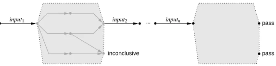
Fig. 6. General structure of a combined test case.
As a consequence of generating multiple acceptance graphs we would over-approxi-mate the possible correct behavior. That means that we consider more observation se-quences to be correct. This follows from the fact that observation sese-quences from dif-ferent acceptance graphs can be combined in any possible order. This would not be possible for a complete input sequence. Consequently, the generation of an acceptance graph should be delayed as much as possible (e.g., in relation to the memory consump-tion). The generated test cases are still sound if the introduction of observation points is valid for the SUT.
Depending on the used testing strategy we can parameterize how test cases should be generated and combined. On the one hand by the effort we need to process the total count of inputs, and on the other hand by the reduction capability when splitting the input sequence into smaller parts. Figure 6 shows the structure of a test case with multi-ple input sequences and corresponding acceptance graphs. When reaching a pass node we continue to trigger the SUT with the next input sequence and check the newly gene-rated output of the SUT at the next observation point. Experiments with this ”static” strategy showed that if we can introduce such observation points for the system un-der test this strategy works quite well. But we also work on more elaborate ”dynamic” strategies (e.g., to take advantage of specific properties of used events of the event store, probabilistic strategies to specify possible event interleavings, or memory and time con-sumption).
3.5 Evaluating the Test Process
If a test suite is generated with the algorithm above and if a SUT is tested with this test suite we would like to know how extensively we tested the system under test. The number of test cases and the length of the input sequences in the test cases only con-ditionally allow to draw conclusions related to that question. Still today the question is hard to answer. The mostly used approach is to measure the coverage of different ele-ments of the system under test or the specification. For program code this is common practice. The used criteria are usually based on control flow or data flow information in the code or on functional description in the specification. With our test approach we address embedded reactive systems composed of hardware and software components. You can apply well known techniques to measure coverage in the software components, but our impression is that this is not sufficient for such systems. To measure coverage in the hardware components is usually not possible. The only way to regard the whole sys-tem is to use the specification. In further work we develop meaningful criteria for state machines. Our current work introduces different criteria based on structural elements
System under Test TCP / IP State Machines Test Suites TCGD Adapter
State Machine Executor
Adapter
Test Driver Test Case Generator
O
O I
I
Fig. 7. Architecture of the TEAGERtool suite.
of state machines, like states and transitions, and on semantic elements, like configura-tions and sets of firing transiconfigura-tions. Especially semantic criteria are able to evaluate the behavior in a more meaningful manner. An interesting question is whether it is possible to use such criteria to control the test case generation process (i.e., to measure coverage while generating test cases and to select the next inputs according to this coverage).
4
Experimental Results
To evaluate our complete test approach we implemented the TEAGERtool suite [29]. TEAGER consists of an environment to automatically generate and execute test cases, and additionally of an environment to execute state machine specifications. We use the latter to analyze the execution behavior and the testability of a state machine, and to measure coverage on a state machine specification to evaluate generated test suites. Figure 7 shows this general architecture. We us the TESTCASEGENERATOR to au-tomatically generate test cases out of a state machine specification. A state machine specification is executed to compute the possible correct observation sequences for se-lected inputs. Based on them an acceptance graph is generated as the test oracle. Input sequences and acceptance graphs are stored for each test case in separate files for later execution. The TESTDRIVERin turn loads saved test cases and executes them. The ex-ecution includes both: stimulating the system under test and comparing the observation to the computed possible correct behavior in the acceptance graphs. The communication with the system under test takes place over a socket connection using pre-implemented adaptors. This concept offers a flexible way to connect the system under test. It also offers the possibility to use our STATEMACHINEEXECUTOR as a system under test stub. Thus we can analyze the execution behavior of state machine specification or measure the coverage of a used specification. The complete test case generation pro-cess is parameterized to have maximal control over the structure of test cases and the effort needed to calculate them. For more information about the TEAGERtool suite, its individual components, and the used parameters, we refer the interested reader to our web site (swt.cs.tu-berlin.de/∼seifert/teager.html).
We applied two case studies on Pentium IV 2.6 GHz to evaluate our test case gener-ation and execution. First, the Car Audio System from Section 2 and second, a system to control the sun blinds of an office building [25]. Generally speaking the results from both case studies allow the same interpretation. In the following, we briefly review some results from the Car Audio System case study to give an impression of the exe-cution behavior of our test approach. We present two different experiments. In the first experiment we demonstrated the exponential calculation effort needed to calculate the
0 2000 4000 6000 8000 10000 12000 14000 0 3 6 9 12 15 18 21 24 27 30
Calculation Time in Seconds
Burst Length test generation test execution 0 200 400 600 800 1000 1200 1400 1600 0 1 2 3 4 5 6 7 8 9 10 11 12 13 14 15 16 Number of combined Bursts
(determ.) burst: 60 (nondeterm.) burst: 11 (car audio system) burst: 15 (car audio system) burst: 17 (more repetitions) burst: 17
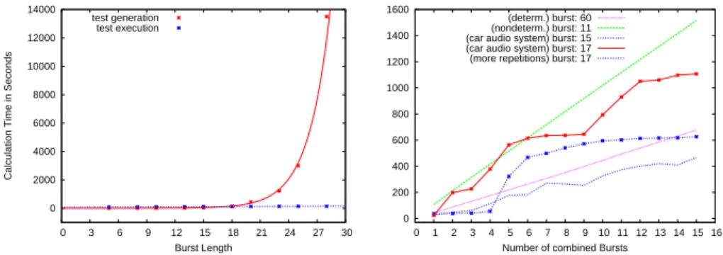
Fig. 8. Results for the first and second experiment.
possible correct observations. In the second experiment we demonstrated the effect of combining multiple input sequences. We used the state machine model from Figure 1 as specification. In all experiments we generated a test suite comprising 25 test cases. In the first experiment we varied the length of the input sequence and in the second ex-periment we fixed the length of the input sequences but varied the number of combined sequences.
Figure 8 illustrates the results of the two experiments. The red graph in the left pic-ture clearly shows the exponential calculation effort of the test generation process. But it also shows that a relatively long input sequence can be processed even for a complex system. The blue graph shows that executing a test case takes considerably less time, and that the time need only slightly increases the longer the input sequences are. From this it follows that the strategy to spend more time in test case generation to generate longer test cases and to save the test cases to be able to execute them multiple times is worthwhile. The blue graph (burst size of 15) and the red graph (burst size of 17) in the right picture visualize the results of the second experiment. The unequal gradients of the subsections in the graphs result from the different calculation effort for the partic-ular inputs (which were selected by a random strategy). To verify this we executed the experiments multiple times and calculated the mean values (the lower blue graph). This graph shows that the generation times converge towards a linear graph. Additionally, we experimented with a deterministic and a non-deterministic specification (the green and magenta graph). The graphs clearly show the expected linear gradient. Finally we mention that the execution effort increases due to the higher number of observation points (which requires to wait for all system reactions). In practice, we need to choose an optimum with respect to the calculation effort and the execution time.
5
Summary and Outlook
Testing benefits from the fact that the actual system is brought to execution. Thus, the interaction of the real hardware and the real software can be evaluated. It is applicable at different levels of abstraction and at different stages of the development. It aims in falsification, that means to show inconsistencies between the specification and the developed system.
Our test approach allows to use UML state machines in quality assurance to pre-cisely specify the reactive behavior of a system, and thus, to serve as the basis for the automated test case generation, execution and evaluation. To generate tests we select relevant input sequences and calculate the possible correct observation sequences for them. Based on these observations we calculate the test oracles which we use to auto-matically evaluate the test executions. Manually performed, this is a difficult and time consuming task. The approximation techniques we applied make the generation pro-cess efficient. It is possible to control the complete propro-cess via parameters depending on the time and computation power you want to invest. The modularization of the tasks gives our approach a clear structure and makes it interesting for further research. All discussed strategies are implemented as modules of the TEAGERtool suite. Thus, dif-ferent strategies for selecting inputs, for combining test cases to reduce the calculation effort, or to select relevant data during test case generations can be studied indepen-dently from each other. Moreover, in practice this allows adaptation to different needs. We use a precisely defined semantics for UML state machines which includes complex structured data. We do not restrict state machines to ease test case generation. Instead, we follow the semantics description of the UML standard [1] as much as possible. Only misleading or conflicting statements are clarified. We address all semantic details which arise from the different sources of non-determinism. In particular we address the problem of asynchronous communication which is introduced by the run-to-completion semantics of state machines. Many real life systems can show such behavior.
Our ongoing research deals with a comprehensive integration of our approach into an UML-based development. In particular we address questions: how to combine our approach with a component-based development approach and how to combine our tech-nics with other successfully applied testing techtech-nics. Furthermore we integrate more and more syntactical elements into our formal semantics and analyze their influence on the automated test generation process. Perspectively we address two challenges, namely specifying and testing timed behavior and considering complex data to generate ”inter-esting” test cases. We also develop techniques to control and evaluate our automated processes. Measuring coverage, especially on the specification, is one step into this di-rection. We are analyzing criteria based on state machines and their semantic model.
References
1. UML2: Unified Modeling Language: Infrastructure and Superstructure. Object Management Group (2007) Version 2.1.1, formal/07-02-03, www.uml.org/uml.
2. Balser, M., B¨aumler, S., Knapp, A., Reif, W., Thums, A.: Interactive Verification of UML State Machines. In: Formal Engineering Methods(ICFEM). LNCS, Springer (2004) 3. Lilius, J., Paltor, I.P.: Formalising UML State Machines for Model Checking. In: The Unified
Modeling Language (UML). LNCS, Springer (1999)
4. Latella, D., Majzik, I., Massink, M.: Automatic Verification of a Behavioural Subset of UML Statechart Diagrams Using the SPIN Model-checker. Formal Aspects of Computing (1999) 5. De Nicola, R., Hennessy, M.C.B.: Testing Equivalences for Processes. Theoretical Computer
Science (1984)
6. Brinksma, E.: A Theory for the Derivation of Tests. In: Protocol Specification, Testing and Verification, North-Holland (1988)
7. Tretmans, J.: Test Generation with Inputs, Outputs and Repetitive Quiescence. Software– Concepts and Tools (1996)
8. Lee, D., Yannakakis, M.: Principles and Methods of Testing Finite State Machines - A Survey. In: Proceedings of the IEEE. (1996)
9. Petrenko, A.: Fault Model-driven Test Derivation from Finite State Models: Annotated Bib-liography. LNCS (2001)
10. Brinksma, E., Tretmans, J.: Testing Transition Systems: An Annotated Bibliography. LNCS (2001)
11. Fujiwara, S., v. Bochmann, G., Khendek, F., Amalou, M., Ghedamsi, A.: Test Selection Based on Finite State Models. IEEE Transactions on Software Engineering (1991)
12. Yang, B., Ural, H.: Protocol Conformance Test Generation using multiple UIO Sequences with Overlapping. SIGCOMM Computer Communication Review (1990)
13. Chow, T.S.: Testing Software Design Modeled by Finite-State Machines. IEEE Transactions on Software Engineering (1978)
14. Luo, G., v. Bochmann, G., Petrenko, A.: Test Selection Based on Communicating Nonde-terministic Finite State Machines Using a Generalized Wp-Method. IEEE Transactions on Software Engineering (1994)
15. Gnesi, S., Latella, D., Massink, M.: Formal Test-case Generation for UML Statecharts. In: Engineering Complex Computer Systems (ICECCS), IEEE Computer Society (2004) 16. Offutt, A.J., Liu, S., Abdurazik, A., Ammann, P.: Generating test data from state-based
specifications. Software Test, Verification. Reliability (2003)
17. Latella, D., Massink, M.: A Formal Testing Framework for UML Statechart Diagrams Be-haviours: From Theory to Automatic Verification. In: International Symposium on High-Assurance Systems Engineering, IEEE Computer Society (2001)
18. Latella, D., Massink, M.: On Testing and Conformance Relations for UML Statechart Dia-grams Behaviours. SIGSOFT Software Engineering Notes (2002)
19. Offutt, J., Abdurazik, A.: Generating Tests from UML Specifications. In: The Unified Modeling Language (UML), Springer (1999)
20. Pretschner, A., L¨otzbeyer, H., Philipps, J.: Model based Testing in incremental System De-velopment. Journal of Systems and Software (2004)
21. Hartman, A., Nagin, K.: The AGEDIS Tools for Model Based Testing. In: International Symposium on Software Testing and Analysis (ISSTA04). (2004) 129–132
22. Campbell, C., Grieskamp, W., Nachmanson, L., Schulte, W., Tillmann, N., Veanes, M.: Model-Based Testing of Object-Oriented Reactive Systems with Spec Explorer. Technical Report MSR-TR-2005-59, Microsoft Research (2005)
23. Harel, D.: Statecharts: A Visual Formulation for Complex Systems. Science of Computer Programming (1987)
24. Seifert, D.: An Executable Formal Semantics for a UML State Machine Kernel Considering Complex Structured Data. Technical Report inria-00274391, DEDALE (LORIA) (2008) 25. Seifert, D.: Automatisiertes Testen asynchroner nichtdeterministischer Systeme mit Daten.
Shaker Verlag (2007) Also: PhD dissertation, Technische Universit¨at Berlin.
26. Harel, D., Naamad, A.: The STATEMATE Semantics of Statecharts. ACM Transactions on Software Engineering and Methodology (1996)
27. De Nicola, R.: Extensional Equivalences for Transition Systems. Acta Informatica (1987) 28. Seifert, D., Souqui`eres, J.: Using UML Protocol State Machines in Conformance Testing of
Components. Technical Report inria-00274383, DEDALE (LORIA) (2008)
29. Santen, T., Seifert, D.: Teager - Test Automation for UML State Machines. In: Software Engineering 2006. LNI, GI (2006)
![Fig. 3. Stepwise state space exploration for the input sequence [a,b,c].](https://thumb-eu.123doks.com/thumbv2/123doknet/12789679.362162/12.918.237.686.163.320/fig-stepwise-state-space-exploration-input-sequence-b.webp)