HAL Id: cea-01709306
https://hal-cea.archives-ouvertes.fr/cea-01709306
Preprint submitted on 14 Feb 2018
HAL is a multi-disciplinary open access
archive for the deposit and dissemination of
sci-entific research documents, whether they are
pub-lished or not. The documents may come from
teaching and research institutions in France or
abroad, or from public or private research centers.
L’archive ouverte pluridisciplinaire HAL, est
destinée au dépôt et à la diffusion de documents
scientifiques de niveau recherche, publiés ou non,
émanant des établissements d’enseignement et de
recherche français ou étrangers, des laboratoires
publics ou privés.
Model Generation for Quantified Formulas: A
Taint-Based Approach
Benjamin Farinier, Sébastien Bardin, Richard Bonichon, Marie-Laure Potet
To cite this version:
Benjamin Farinier, Sébastien Bardin, Richard Bonichon, Marie-Laure Potet. Model Generation for
Quantified Formulas: A Taint-Based Approach. 2018. �cea-01709306�
Model Generation for Quantified Formulas:
A Taint-Based Approach
Benjamin Farinier1,2, Sébastien Bardin1,
Richard Bonichon1, and Marie-Laure Potet2
1 CEA, LIST, Software Safety and Security Lab, Université Paris-Saclay, France
2 Univ. Grenoble Alpes, Verimag, France
Abstract. We focus in this paper on generating models of quantified
first-order formulas over built-in theories, which is paramount in software verification and bug finding. While standard methods are either geared toward proving the absence of solution or targeted to specific theories, we propose a generic approach based on a reduction to the quantifier-free case. Our technique allows thus to reuse all the efficient machinery developed for that context. Experiments show a substantial improvement over state-of-the-art methods.
Keywords: automated reasoning; first-order logic; model generation
1
Introduction
Context. Software verification methods have come to rely increasingly on
rea-soning over logical formulas modulo theory. In particular, the ability to generate models (i.e., find solutions) of a formula is of utmost importance, typically in the context of bug finding or intensive testing — symbolic execution [19] or bounded model checking [7]. Since quantifier-free first-order formulas on well-suited theo-ries are sufficient to represent many reachability properties of interest, the Satis-fiability Modulo Theory (SMT) [6,22] community has primarily dedicated itself to designing solvers able to efficiently handle such problems.
Yet, universal quantifiers are sometimes needed, typically when considering preconditions or code abstraction. Unfortunately, most theories handled by SMT-solvers are undecidable in the presence of universal quantifiers. There exist ded-icated methods for a few decidable quantified theories, such as Presburger arith-metic [9] or the array property fragment [8], but there is no general and effective enough approach for the model generation problem over universally quantified formulas. Indeed, generic solutions for quantified formulas involving heuristic in-stantiation and refutation are geared at proving the unsatisfiability of a formula (i.e., absence of solution) [12,18], while recent proposals such as local theory extensions [2], finite instantiation [27,28] or model-based instantiation [25,18] ei-ther are too narrow in scope, or handle quantifiers on free sorts only, or restrict themselves to finite models, or may get stuck in infinite refinement loops.
Goal and challenge. Our goal is to propose a generic and efficient approach to
the model generation problem over arbitrary quantified formulas with support for theories commonly found in software verification. Due to the huge effort made by the community to produce state-of-the-art solvers for quantifier-free theories (QF-solvers), it is highly desirable for this solution to be compatible with current
leading decision procedures, namely SMT approaches.
Proposal. Our approach turns a quantified formula into a quantifier-free
for-mula with the guarantee that any model of the later contains a model of the former. The benefits are threefold: the transformed formula is easier to solve, it can be sent to standard QF-solvers, and a model for the initial formula is deducible from a model of the transformed one. The idea is to ignore quanti-fiers but strengthen the quantifier-free part of the formula with an independence
condition constraining models to be independent from the (initially) quantified
variables.
Contributions. This paper makes the following contributions:
We propose a novel and generic framework for model generation of quantified formula (Sec. 5, Alg. 1) relying on the inference of sufficient independence
con-dition (Sec. 4). We prove its correctness (Thm. 1, mechanized in Coq) and its efficiency under reasonable assumptions (Prop. 4 and 5). Especially our
ap-proach implies only a linear overhead in the formula size. We also briefly study its completeness, related to the notion of weakest independence condition. We define a taint-based procedure for the inference of independence
condi-tions (Sec. 5.2), composed of a theory-independent core (Alg. 2) together with theory-dependent refinements. We propose such refinements for a large class of operators (Sec. 6.2), encompassing notably arrays and bitvectors.
Finally, we present a concrete implementation of our method specialized on arrays and bitvectors (Sec. 7). Experiments on SMT-LIB benchmarks and software verification problems demonstrate that we are able not only to very effectively lift quantifier-free decision procedures to the quantified case, but also to supplement recent advances, such as finite or model-based quantifier instantiation [27,28,25,18]. Indeed, we concretely supply SMT solvers with the ability to efficiently address an extended set of software verification questions.
Discussions. Our approach supplements state-of-the-art model generation on
quantified formulas by providing a more generic handling of satisfiable problems. We can deal with quantifiers on any sort and we are not restricted to finite mod-els. Moreover, this is a lightweight preprocessing approach requiring a single call to the underlying quantifier-free solver. The method also extends to partial elimination of universal quantifiers, or reduction to quantified-but-decidable for-mulas (Sec. 5.4). While techniques a la E-matching allow to lift quantifier-free solvers to the unsatisfiability checking of quantified formulas, this works provides a mechanism to lift them to the satisfiability checking and model generation of quantified formulas, yielding a more symmetric handling of quantified formulas in SMT. This new approach paves the way to future developments such as the definition of more precise inference mechanisms of independence conditions, the
identification of subclasses for which inferring weakest independence conditions is feasible, and the combination with other quantifier instantiation techniques.
2
Motivation
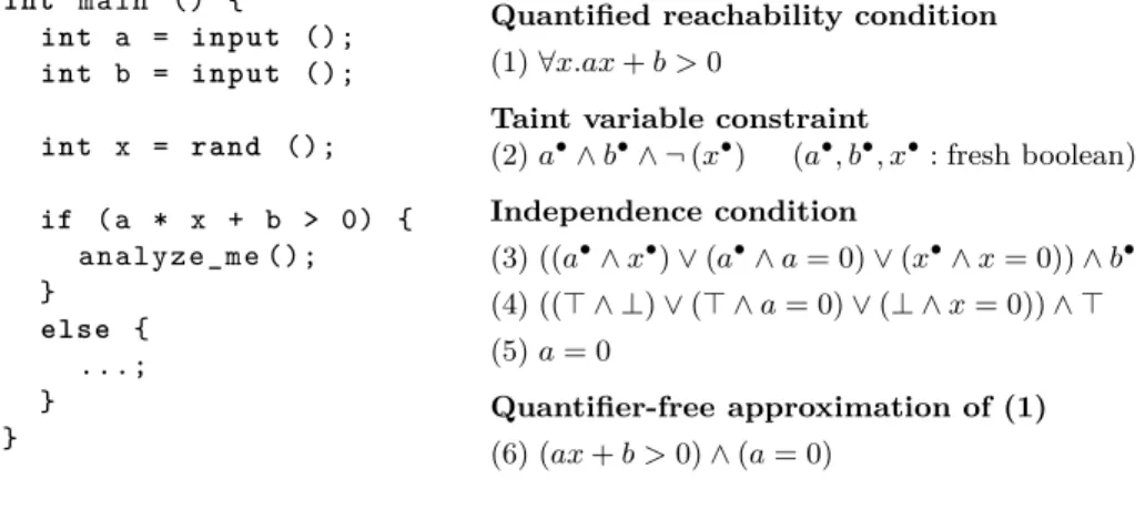
Let us take the code sample in Fig. 1 and suppose we want to reach function analyze_me. For this purpose, we need a model (a.k.a., solution) of the reachabil-ity condition φ, ax + b > 0, where a, b and x are symbolic variables associated to the program variables a, b and x. However, while the values of a and b are user-controlled, the value of x is not. Therefore if we want to reach analyze_me in a reproducible manner, we actually need a model of φ∀, ∀x.ax + b > 0, which
involves universal quantification. While this specific formula is simple, model
generation for quantified formulas is notoriously difficult: PSPACE-complete for booleans, undecidable for uninterpreted functions or arrays.
int main () { int a = input (); int b = input (); int x = rand (); if ( a * x + b > 0) { analyze_me (); } else { ...; } }
Quantified reachability condition
(1) ∀x.ax + b > 0
Taint variable constraint
(2) a•∧ b•∧ ¬ (x•) (a•, b•, x•: fresh boolean) Independence condition (3) ((a•∧ x•) ∨ (a•∧ a = 0) ∨ (x•∧ x = 0)) ∧ b• (4) ((⊤ ∧ ⊥) ∨ (⊤ ∧ a = 0) ∨ (⊥ ∧ x = 0)) ∧ ⊤ (5) a = 0 Quantifier-free approximation of (1) (6) (ax + b > 0) ∧ (a = 0)
Fig. 1: Motivating example
Reduction to the quantifier-free case through independence. We
pro-pose to ignore the universal quantification over x, but restrict models to those
which do not depend on x. For example, model {a = 1, x = 1, b = 0} does depend
on x, as taking x = 0 invalidates the formula, while model {a = 0, x = 1, b = 1} is independent of x. We call constraint ψ, (a = 0) an independence condition: any interpretation of φ satisfying ψ will be independent of x, and therefore a model of φ ∧ ψ will give us a model of φ∀.
Inference of independence conditions through tainting. Fig. 1 details in
its right part a way to infer such independence conditions. Given a quantified reachability condition (1), we first associate to every variable v a (boolean) taint
variable v• indicating whether the solution may depend on v (value ⊤) or not
(value ⊥). Here, x• is set to ⊥, a• and b• are set to ⊤ (2). An independence
condition (3) — a formula modulo theory — is then constructed using both initial and taint variables. We extend taint constraints to terms, t• indicating
(i.e., the formula) to be tainted to ⊤ (i.e., to be indep. from x). Condition (3) reads as follows: in order to enforce that (ax + b > 0)• holds, we enforce that
(ax)• and b• hold, and for (ax)• we require that either a• and x• hold, or a•
holds and a = 0 (absorbing the value of x), or the symmetric case. We see that ·• is defined recursively and combines a systematic part (if t• holds then
f(t)• holds, for any f ) with a theory-dependent part (here, based on ×). After
simplifications (4), we obtain a = 0 as an independence condition (5) which is adjoined to the reachability condition freed of its universal quantification (6). A QF-solver provides a model of (6) (e.g., {a = 0, b = 1, x = 5}), lifted into a model of (1) by discarding the valuation of x (e.g., {a = 0, b = 1}).
In this specific example the inferred independence condition (5) is the most generic one and (1) and (6) are equisatisfiable. Yet, in general it may be an under-approximation, constraining the variables more than needed and yielding a correct but incomplete decision method: a model of (6) can still be turned into a model of (1), but (6) might not have a model while (1) has.
3
Notations
We consider the framework of many-sorted first-order logic with equality, and we assume standard definitions of sorts, signatures and terms. Given a tuple of variables x, (x1, . . . , xn) and a quantifier Q (∀ or ∃), we shorten Qx1. . .Qxn.Φ
as Qx.Φ. A formula is in prenex normal form if it is written as Q1x1. . .Qnxn.Φ
with Φ a quantifier-free formula. A formula is in Skolem normal form if it is in prenex normal form with only universal quantifiers. We write Φ (x) to denote that the free variables of Φ are in x. Let t , (t1, . . . , tn) be a term tuple, we
write Φ (t) for the formula obtained from Φ by replacing each occurrence of xi
in Φ by ti. An interpretation I associates a domain to each sort of a signature
and a value to each symbol of a formula, and J∆KI denotes the evaluation of
term ∆ over I. A satisfiability relation |= between interpretations and formulas is defined inductively as usual. A model of Φ is an interpretation I satisfying I |= Φ. We sometimes refer to models as “solutions”. Formula Ψ entails formula
Φ, written Ψ |= Φ, if every interpretation satisfying Ψ satisfies Φ as well. Two formula are equivalent, denoted Ψ ≡ Φ, if they have the same models. A theory T , (Σ, I) restricts symbols in Σ to be interpreted in I. The quantifier-free fragment of T is denoted QF-T .
Convention. Letters a, b, c . . . denote uninterpreted symbols and variables.
Let-ters x, y, z . . . denote quantified variables. a, b, c denote sets of uninterpreted symbols. x, y, z . . . denote sets of quantified variables. Finally, a, b, c . . . denote valuations of associated (sets of) symbols.
In the rest of this paper, we assume w.l.o.g. that all formulas are in Skolem normal form. Recall that any formula φ in classical logic can be normalized into a formula ψ in Skolem normal form such that any model of φ can be lifted into a model of ψ, and vice versa. This strong relation, much closer to formula equivalence than to formula equisatisfiability, ensures that our correctness and completeness results all along the paper hold for arbitrarily quantified formula.
Appendix. Additional technical details (proofs, experiments, etc.) are provided
in appendix. This content will be made available in an online technical report.
4
Musing with independence
4.1 Independent interpretations, terms and formulas
A solution (x, a) of Φ does not depend on x if Φ(x, a) is always true or always false, for all possible valuations of x as long as a is set to a. More formally, we define the independence of an interpretation of Φ w.r.t. x as follows:
Definition 1 (Independent interpretation).
– Let Φ (x, a) a formula with free variables x and a. Then an interpretation I
of Φ (x, a) is independent of x if for all interpretations J equal to I except on x, I |= Φ if and only if J |= Φ.
– Let ∆ (x, a) a term with free variables x and a. Then an interpretation I
of ∆ (x, a) is independent of x if for all interpretations J equal to I except on x, J∆ (x, a)KI = J∆ (x, a)KJ.
Regarding formula ax + b > 0 from Fig. 1, {a = 0, b = 1, x = 1} is indepen-dent of x while {a = 1, b = 0, x = 1} is not. Considering term (t [a ← b]) [c], with
tan array written at index a then read at index c, {a = 0, b = 42, c = 0, t = [. . . ]} is independent of t (evaluates to 42) while {a = 0, b = 1, c = 2, t = [. . . ]} is not (evaluates to t [2]). We now define independence for formulas and terms.
Definition 2 (Independent formula and term).
– Let Φ (x, a) a formula with free variables x and a. Then Φ (x, a) is
indepen-dent of x if ∀x.∀y. (Φ (x, a) ⇔ Φ (y, a)) holds true for any value of a.
– Let ∆ (x, a) a term with free variables x and a. Then ∆ (x, a) is independent
of x if ∀x.∀y. (∆ (x, a) = ∆ (y, a)) holds true for any value of a.
Def. 2 of formula and term independence is far stronger than Def. 1 of in-terpretation independence. Indeed, it can easily be checked that if a formula Φ (resp. a term ∆) is independent of x, then any interpretation of Φ (resp. ∆) is independent of x. However, the converse is false as formula ax + b > 0 is not independent of x, but has an interpretation {a = 0, b = 1, x = 1} which is.
4.2 Independence conditions
Since it is rarely the case that a formula (resp. term) is independent from a set of variables x, we are interested in Sufficient Independence Conditions. These conditions are additional constraints that can be added to a formula (resp. term) in such a way that they make the formula (resp. term) independent of x.
Definition 3 (Sufficient Independence Condition (SIC)).
– A Sufficient Independence Condition for a formula Φ (x, a) with regard to x
– A Sufficient Independence Condition for a term ∆ (x, a) with regard to x, is
a formula Ψ (a) such that Ψ (a) |= (∀x.∀y.∆ (x, a) = ∆ (y, a)).
We denote by sicΦ,x (resp. sic∆,x) a Sufficient Independence Condition for
a formula Φ (x, a) (resp. for a term ∆ (x, a)) with regard to x. For example,
a = 0 is a sicΦ,x for formula Φ , ax + b > 0, and a = c is a sic∆,t for term
∆, (t [a ← b]) [c]. Note that ⊥ is always a sic, and that sic are closed under ∧ and ∨. Prop. 1 clarifies the interest of sic for model generation.
Proposition 1 (Model generalization). Let Φ (x, a) a formula and Ψ a sicΦ,x.
If there exists an interpretation {x, a} such that {x, a} |= Ψ (a) ∧ Φ (x, a), then
{a} |= ∀x.Φ (x, a).
Proof (sketch of). Appendix C.1.
For the sake of completeness, we introduce now the notion of Weakest
In-dependence Condition for a formula Φ (x, a) with regard to x (resp. a term ∆(x, a)). We will denote such conditions wicΦ,x (resp. wic∆,x).
Definition 4 (Weakest Independence Condition (WIC)).
– A Weakest Independence Condition for a formula Φ (x, a) with regard to x
is a sicΦ,x Π such that, for any other sicΦ,x Ψ, Ψ |= Π.
– A Weakest Independence Condition for a term ∆ (x, a) with regard to x is
a sic∆,x Π such that, for any other sic∆,x Ψ, Ψ |= Π.
Note that Ω , ∀x.∀y. (Φ (x, a) ⇔ Φ (y, a)) is always a wicΦ,x, and any
formula Π is a wicΦ,x if and only if Π ≡ Ω. Therefore all syntactically different
wichave the same semantics. As an example, both sic a = 0 and a = c presented earlier are wic. Prop. 2 emphasizes the interest of wic for model generation.
Proposition 2 (Model specialization). Let Φ (x, a) a formula and Π(a) a
wicΦ,x. If there exists an interpretation {a} such that {a} |= ∀x.Φ (x, a), then
{x, a} |= Π (a) ∧ Φ (x, a) for any valuation x of x.
Proof (sketch of). Appendix C.2.
From now on, our goal is to infer from a formula ∀x.Φ (x, a) a sicΦ,x Ψ(a),
find a model for Ψ (a) ∧ Φ (x, a) and generalize it. This sicΦ,xshould be as weak
— in the sense “less coercive” — as possible, as otherwise ⊥ could always be used, which would not be very interesting for our overall purpose.
For the sake of simplicity, previous definitions omit to mention the theory to which the sic belongs. If the theory T of the quantified formula is decidable we can always choose ∀x.∀y. (Φ (x, a) ⇔ Φ (y, a)) as a sic, but it is simpler to directly use a T -solver. The challenge is, for formulas in an undecidable theory T , to find a non-trivial sic in its quantifier-free fragment QF-T .
Under this constraint, we cannot expect a systematic construction of wic, as it would allow to decide the satisfiability of any quantified theory with a decidable quantifier-free fragment. Yet informally, the closer a sic is to be a wic, the closer our approach is to completeness. Therefore this notion might be seen as a fair gauge of the quality of a sic. Having said that, we leave a deeper
5
Generic framework for SIC-based model generation
We describe now our overall approach. Alg. 1 presents our sic-based generic framework for model generation (Sec. 5.1). Then, Alg. 2 proposes a taint-based approach for sic inference (Sec. 5.2). Finally, we discuss complexity and effi-ciency issues (Sec. 5.3) and detail extensions (Sec. 5.4), such as partial elimina-tion.
From now on, we do not distinguish anymore between terms and formulas, their treatment being symmetric, and we call targeted variables the variables we want to be independent of.
5.1 SIC-based model generation
Algorithm 1: SIC-based model generation for quantified formulas
Parameter: solveQF
Input: Φ(v) a formula in QF-T
Output: sat (v) with v |= Φ, unsat or unknown Parameter: inferSIC
Input: Φ a formula in QF-T , and x a set of targeted variables
Output: Ψ a sicΦ,xin QF-T
Function solveQ:
Input: ∀x.Φ (x, a) a universally quantified formula over theory T Output: sat (a) with a |= ∀x.Φ (x, a), unsat or unknown
Let Ψ (a), inferSIC (Φ (x, a) , x)
match solveQF (Φ (x, a) ∧ Ψ (a)) with sat (x, a) return sat (a) with unsat
if Ψ is a wicΦ,xthen return unsat
else return unknown with unknown return unknown
Our model generation technique is described in Alg. 1. Function solveQ takes as input a formula ∀x.Φ (x, a) over a theory T . It first calculates a sicΦ,x Ψ(a)
in QF-T . Then it solves Φ (x, a) ∧ Ψ (a). Finally, depending on the result and whether Ψ (a) is a wicΦ,x or not, it answers sat, unsat or unknown. solveQ
is parametrized by two functions solveQF and inferSIC:
– solveQF is a decision procedure (typically a SMT solver) for QF-T . solveQF
is said to be correct if each time it answers sat (resp. unsat) the formula is satisfiable (resp. unsatisfiable); it is said to be complete if it always answers sator unsat, never unknown.
– inferSIC takes as input a formula Φ in QF-T and a set of targeted variables x, and produces a sicΦ,xin QF-T . It is said to be correct if it always returns a
sic, and complete if all the sic it returns are wic. A possible implementation of inferSIC is described in Alg. 2 (Sec. 5.2).
Function solveQ enjoys the two following properties, where correctness and com-pleteness are defined as for solveQF.
Theorem 1 (Correctness and completeness).
– If solveQF and inferSIC are correct, then solveQ is correct. – If solveQF and inferSIC are complete, then solveQ is complete.
Proof (sketch of). Follow directly from Prop. 1 and 2 (Sec. 4.2).
5.2 Taint-based SIC inference Algorithm 2: Taint-based sic inference
Parameter: theorySIC
Input: f a function symbol, its parameters φi, x a set of targeted variables
and ψi their associated sicφi,x
Output: Ψ a sicf(φi),x
Default: Return ⊥ Function inferSIC(Φ,x):
Input: Φ a formula and x a set of targeted variables
Output: Ψ a sicΦ,x
either Φ is a constant return ⊤
either Φ is a variable v return v /∈ x
either Φ is a function f (φ1, . , φn)
Let ψi, inferSIC (φi, x) for all i ∈ {1, . , n}
Let Ψ , theorySIC (f, (φ1,., φn) , (ψ1,., ψn) , x)
return Ψ ∨Viψi
Alg. 2 presents a taint-based implementation of function inferSIC. It con-sists in a (syntactic) core calculus described here, refined by a (semantic) theory-dependent calculus theorySIC described in Sec. 6. From formula Φ (x, a) and targeted variables x, inferSIC is defined recursively as follow.
If Φ is a constant it returns ⊤ as constants are independent of any variable. If Φ is a variable v, it returns ⊤ if we may depend on v (i.e., v 6∈ x), ⊥ otherwise. If Φ is a function f (φ1, . , φn), it first recursively computes for every sub-term φi
a sicφi,x ψi. Then these results are sent with Φ to theorySIC which computes a sicΦ,x Ψ. The procedure returns the disjunction between Ψ and the conjunction
of the ψi’s. Note that theorySIC default value ⊥ is absorbed by the disjunction.
The intuition is that if the φi’s are independent of x, then f (φ1, . , φn) is.
Therefore Alg. 2 is said to be taint-based as, when theorySIC is left to its default value, it acts as a form of taint tracking [14,24] inside the formula.
Proposition 3 (Correctness). Given a formula Φ (x, a) and assuming that
theorySICis correct, then inferSIC (Φ, x) indeed computes a sicΦ,x.
Proof (sketch of). This proof has been mechanized in Coq.
Note that on the other hand, completeness does not hold: in general inferSIC does not compute a wic, cf. discussion in Sec. 5.4.
5.3 Complexity and efficiency
We now evaluate the overhead induced by Alg. 1 in terms of formula size and complexity of the resolution — the running time of Alg. 1 itself being expected to be negligible (preprocessing).
Definition 5. The size of a term is inductively defined as size (x) , 1 for
x a variable, and size (f (t1, . , tn)) , 1 + Σisize (ti) otherwise. We say that
theorySICis bounded in size if there exists K such that, for all term ∆, size (theorySIC (∆, ·)) ≤ K.
Proposition 4 (Size bound). Let N be the maximal arity of symbols defined
by theory T . If theorySIC is bounded in size by K, then for all formula Φ in T , size (inferSIC (Φ, ·)) ≤ (K + N ) · size (Φ).
Proposition 5 (Complexity bound). Let us suppose theorySIC bounded in
size, and let Φ be a formula belonging to a theory T with polynomial-time check-able solutions. If Ψ is a sicΦ,· produced by inferSIC, then a solution for Φ ∧ Ψ
is checkable in time polynomial in size of Φ. Proof (sketch of). Appendices C.3 and C.4
These propositions demonstrate that, for formula landing in complex enough theories, our method lifts QF-solvers to the quantified case (in an approximated way) without any significant overhead, as long as theorySIC is bounded in size. This later constraint can be achieved by systematically binding sub-terms to (constant-size) fresh names and having theorySIC manipulates these binders.
5.4 Discussions
Extension. Let us remarks that our framework encompasses partial quantifier
elimination as long as the remaining quantifiers are handled by solveQF. For example, we may want to remove quantifications over arrays but keep those on bitvectors. In this setting, inferSIC can also allow some level of quantification, providing that solveQF handles them.
About WIC. As already stated, inferSIC does not propagate wic in
gen-eral. For example, considering formulas t1 , (x < 0) and t2 , (x ≥ 0), then
wict1,x= ⊥ and wict2,x= ⊥. Hence inferSIC returns ⊥ as sic for t1∨ t2, while
actually wict1∨t2,x = ⊤. As a second example, let us consider term f (a, x) with
f uninterpreted. Then wicf(a,x),x= ⊤ while inferSIC returns ⊥.
Nevertheless, we can already highlight a few cases where wic can be com-puted. inferSIC does propagate wic on one-to-one uninterpreted functions. If no variable x is present in a sub-term, then the associated wic is ⊤. While a priori naive, this case becomes interesting when combined with simplifications (Sec. 7.1) that may eliminate x. If a sub-term falls in a sub-theory admitting quantifier elimination, then the associated wic is computed by eliminating quan-tifiers in (∀.x.y.Φ(x, a) ⇔ Φ(y, a)). We may also think of dedicated patterns:
regarding bitvectors, the wic for x ≤ a ∧ x ≤ x + k is a ≤ Max − k.
Identify-ing under which condition wic propagation holds is a strong direction for future work.
6
Theory-dependent SIC refinements
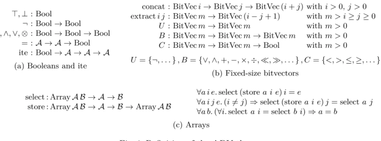
We now present theory-dependent sic refinements for theories relevant to pro-gram analysis: booleans, fixed-size bitvectors and arrays — recall that uninter-preted functions are already handled by Alg. 2. We then propose a generalization of these refinements together with a correctness proof for a larger class of oper-ators.
6.1 Refinement on theories
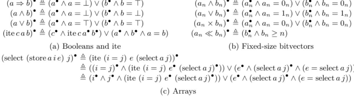
We recall theorySIC takes four parameters: a function symbol f , its arguments (t1, . , tn), their associated sic (t•1, . , t•n), and targeted variables x. theorySIC
pattern-matches the function symbol and returns the associated sic according to rules in Fig. 2. If a function symbol is not supported, we return default value ⊥. Constants and variables are handled by inferSIC. For the sake of simplicity, rules in Fig. 2 are defined recursively, but can easily fit the interface required for theorySICin Alg. 2 by turning recursive calls into parameters.
Booleans and ite. Rules for the boolean theory (Fig. 2a) handles ⇒, ∧, ∨
and ite (if-then-else). For binary operators, the sic is the conjunction of the sic associated to one of the two sub-terms and a constraint on this sub-term that forces the result of the operator to be constant — e.g., to be equal to ⊥ (resp. ⊤) for the antecedent (resp. consequent) of an implication. These equality
constraints are based on absorbing elements of operators.
Inference for the ite operator is more subtle. Intuitively, if its condition is independent of some x, we use it to select the sicx of the sub-term that will be selected by the ite operator. If the condition is dependent of x, then we cannot use it anymore to select a sicx. In this case, we return the conjunction of the sicx of both sub-terms and the constraint that the two sub-terms are equal. Bitvectors and arrays. Rules for bitvectors (Fig. 2b) follow similar ideas, with
constant ⊤ (resp. ⊥) substituted by 1n (resp. 0n), the bitvector of size n full of
ones (resp. zeros). Rules for arrays (Fig. 2c) are derived from the theory axioms. The definition is recursive: rules need be applied until reaching either a store at the position where the select occurs, or the initial array variable.
As a rule of thumb, good sic can be derived from function axioms in the form of rewriting rules, as done for arrays. Similar constructions can be obtained for example for stacks or queues.
6.2 R-absorbing functions
We propose a generalization of the previous theory-dependent sic refinements to a larger class of functions, and prove its correctness.
(a ⇒ b)•, (a•∧ a = ⊥) ∨ (b•∧ b = ⊤)
(a ∧ b)•, (a•∧ a = ⊥) ∨ (b•∧ b = ⊥)
(a ∨ b)•, (a•∧ a = ⊤) ∨ (b•∧ b = ⊤)
(ite c a b)•, (c•∧ ite c a•b•) ∨ (a•∧ b•∧ a = b)
(a) Booleans and ite
(an∧ bn)•, (a•n∧ an= 0n) ∨ (b•n∧ bn= 0n)
(an∨ bn)•, (a•n∧ an= 1n) ∨ (b•n∧ bn= 1n)
(an× bn)•, (a•n∧ an= 0n) ∨ (b•n∧ bn= 0n)
(an≪ bn)•, (b•n∧ bn≥ n)
(b) Fixed-size bitvectors (select (store a i e) j)•, (ite (i = j) e (select a j))•
, ((i = j)•∧ (ite (i = j) e•(select a j)•)) ∨ (e•∧ (select a j)•∧ (e = select a j))
, (i•∧ j•∧ (ite (i = j) e•(select a j)•)) ∨ (e•∧ (select a j)•∧ (e = select a j))
(c) Arrays
Fig. 2: Examples of refinements for theorySIC
Intuitively, if a function has an absorbing element, constraining one of its operands to be equal to this element will ensure that the result of the function is independent of the other operands. However, it is not enough when a relation between some elements is needed, such as with (t[a ← b]) [c] where constraint
a= c ensures the independence with regards to t. We thus generalize the notion of absorption to R-absorption, where R is a relation between function arguments.
Definition 6. Let f : τ1× · · · × τn → τ a function. f is R-absorbing if there
exists IR⊂ {1, · · · , n} and R a relation between αi: τi, i∈ IR such that, for all
b, (b1, . . . , bn) and c, (c1, . . . , cn) ∈ τ1× · · · × τn, if R( b|IR) and b|IR = c|IR
where ·|IR is the projection on IR, then f (b) = f (c).
IR is called the support of the relation of absorption R.
For example, (a, b) 7→ a ∨ b has two pairs hR, IRi coinciding with the usual
notion of absorption, ha = ⊤, {1a}i and hb = ⊤, {2b}i. Function (x, y, z) 7→ xy + z
has among others the pair hx = 0, {1x,3z}i, while (a, b, c, t) 7→ (t[a ← b]) [c] has
the pair ha = c, {1a,3c}i. We can now state the following proposition:
Proposition 6. Let f (t1, . . . , tn) be a R-absorbing function of support IR, and
let t•
i be a sicti,x for some x. Then R (ti∈IR)
V
i∈IRt
•
i is a sicf,x.
Proof (sketch of). Appendix C.5
Previous examples (Sec. 6.1) can be recast in term of R-absorbing function, proving their correctness (Fig. 5 in Appendix B.2). Note also that regarding our end-goal, we should accept only R-absorbing functions in QF-T .
7
Experimental evaluation
This section describes the implementation of our method (Sec. 7.1) for bitvectors and arrays (ABV), together with experimental evaluation (Sec. 7.2).
7.1 Implementation
Our prototype Tfml (Taint engine for ForMuLa) comprises 7 klocs of OCaml. Given an input formula in the SMT-LIB format [5] (ABV theory), Tfml per-forms several normalizations before adding taint information following Alg. 1. The process ends with simplifications as taint usually introduces many constant values, and a new SMT-LIB formula is output.
Sharing with let-binding. This stage is crucial as it allows to avoid term
du-plication in theorySIC (Alg. 2, Sec. 5.3, and Prop. 4). We introduce new names for relevant sub-terms in order to easily share them.
Simplifications. We perform constant propagation and rewriting (standard
rules, e.g. x − x 7→ 0 or x × 1 7→ x) on both initial and transformed formulas – equality is soundly approximated by syntactic equality.
Shadow arrays. We encode taint constraints over arrays through shadow arrays.
For each array declared in the formula, we declare a (taint) shadow array. The default value for all cells of the shadow array is the taint of the original array, and for each value stored (resp. read) in the original array, we store (resp. read) the taint of the value in the shadow array. As logical arrays are infinite, we cannot constraint all the values contained in the initial shadow array. Instead, we rely on a common trick in array theory: we constraint only cells corresponding to a relevant read index in the formula.
Iterative skolemization. While we have supposed along the paper to work on
skolemized formulas, we have to be more careful in practice. Indeed, skolemiza-tion introduce dependencies between a skolemized variable and all its preceding universally quantified variables, blurring our analysis and likely resulting in con-sidering the whole formula as dependent. Instead, we follow an iterative process: 1. Skolemize the first block of existentially quantified variables; 2. Compute the independence condition for any targeted variable in the first block of universal quantifiers and remove these quantifiers; 3. Repeat. This results in full Skolemiza-tion together with the construcSkolemiza-tion of an independence condiSkolemiza-tion, while avoiding many unnecessary dependencies.
7.2 Evaluation
Objective. We experimentally evaluate the following research questions: RQ1 How
does our approach perform with regard to state-of-the-art approaches for model generation of quantified formulas? RQ2 How effective is it at lifting quanti-fier-free solvers into (sat-only) quantified solvers? RQ3 How efficient is it in terms of preprocessing time and formula size overhead? We evaluate our method on a set of formulas combining arrays and bitvectors (paramount in software verification), against state-of-the-art solvers for these theories.
Protocol. The experimental setup below runs on an Intel(R) Xeon(R) E5-2660
Metrics For RQ1 we compare the number of sat and unknown answers
between solvers supporting quantification, with and without our approach. For RQ2 , we compare the number of sat and unknown answers between quantifier-free solvers enhanced by our approach and solvers supporting quan-tification. For RQ3 , we measure preprocessing time and formulas size over-head.
Benchmarks We consider two sets of ABV formulas. First, a set of 1421
formu-las from (a modified version of) the symbolic execution tool Binsec [11] rep-resenting quantified reachability queries (cf. Sec. 2) over Binsec benchmark programs (security challenges, e.g. crackme or vulnerability finding). The ini-tial (array) memory is quantified so that models depend only on user input. Second, a set of 1269 ABV formulas generated from formulas of the QF-ABV category of SMT-LIB [5] – sub-categories brummayerbiere, dwp formulas and klee selected. The generation process consists in universally quanti-fying some of the initial array variables, mimicking quantified reachability problems.
Competitors For RQ1 , we compete against the two state-of-the-art SMT solvers
for quantified formulas CVC4 [4] (finite model instantiation [27]) and Z3 [13] (mode-based instantiation [18]). We also consider degraded versions CVC4E
and Z3E that roughly represent standard E-matching [15]. For RQ2 we use
Boolector [10], one of the very best QF-ABV solvers.
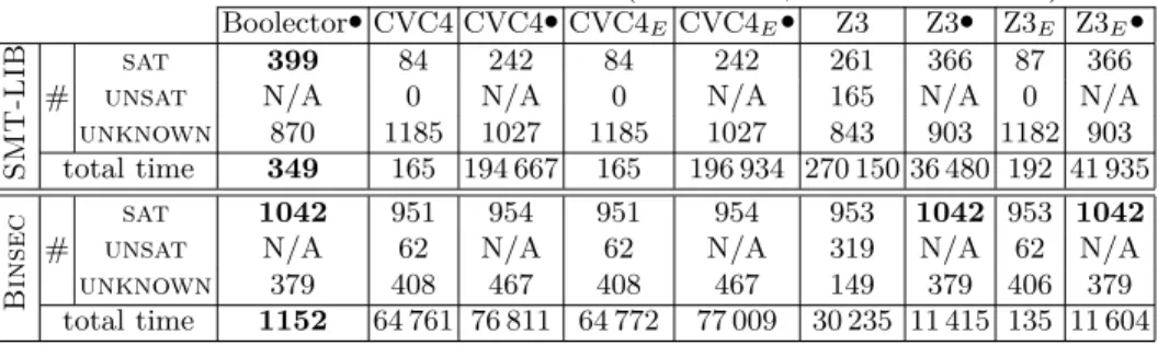
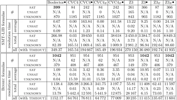
Table 1: Answers and resolution time (in seconds, include timeout)
Boolector• CVC4 CVC4• CVC4ECVC4E• Z3 Z3• Z3E Z3E• S M T -L IB sat 399 84 242 84 242 261 366 87 366
# unsat N/A 0 N/A 0 N/A 165 N/A 0 N/A unknown 870 1185 1027 1185 1027 843 903 1182 903 total time 349 165 194 667 165 196 934 270 150 36 480 192 41 935 B in s e c sat 1042 951 954 951 954 953 1042 953 1042
# unsat N/A 62 N/A 62 N/A 319 N/A 62 N/A unknown 379 408 467 408 467 149 379 406 379 total time 1152 64 761 76 811 64 772 77 009 30 235 11 415 135 11 604 solver•: solver enhanced with our method Z3E, CVC4E: essentially E-matching
Results. Tables 1 and 2 and Fig. 3 sum up our experimental results, which have
all been cross-checked for consistency. Table 1 reports the number of successes (sat or unsat) and failures (unknown), plus total solving times (average time in Appendix D). The • sign indicates formulas preprocessed with our approach. In that case it is impossible to correctly answer unsat (no wic checking), the unsat line is thus N/A. Since Boolector do not support quantified ABV formulas, we only give results with our approach enabled. Table 1 reads as follow: of the 1269 SMT-LIB formulas, standalone Z3 solves 426 formulas (261 sat, 165 unsat), and 366 (all sat) if preprocessed. Interestingly, our approach always improves
the underlying solver in terms of solved (sat) instances, either in a significant way (SMT-LIB) or in a modest way (Binsec). Yet, recall that in a software verification setting every win matters (possibly new bug found or new assertion proved). For Z3•, it also strongly reduces computation time. Last but not least, Boolector• (a pure QF-solver) turns out to have the best performance on sat-instances, beating state-of-the-art approaches both in terms of solved instances and computation time.
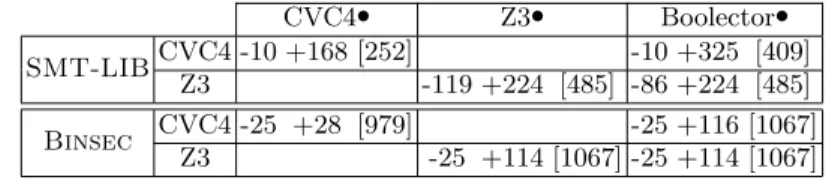
Table 2 substantiates the complementarity of the different methods, and reads as follow: for SMT-LIB, Boolector• solves 224 (sat) formulas missed by Z3, while Z3 solves 86 (sat) formulas missed by Boolector•, and 485 (sat) formulas are solved by either one of them.
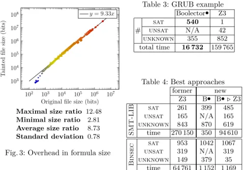
Fig. 3 shows formula size averaging a 9-fold increase (min 3, max 12): yet they are easier to solve because more constrained. Regarding performance and overhead of the tainting process, taint time is almost always less than 1s in our experiments (not shown here), 4min for worst case, clearly dominated by resolution time. The worst case is due to a pass of linearithmic complexity which can be optimized to be logarithmic.
Table 2: Complementarity of our approach with existing solvers (sat instances)
CVC4• Z3• Boolector• SMT-LIBCVC4 -10 +168 [252] -10 +325 [409]
Z3 -119 +224 [485] -86 +224 [485] Binsec CVC4 -25 +28 [979] -25 +116 [1067]
Z3 -25 +114 [1067] -25 +114 [1067]
Pearls. We show hereafter two particular applications of our method. Table 3
reports results of another symbolic execution experiment, on the grub example. On this example, Boolector• completely outperforms existing approaches. As a second application, while the main drawback of our method is that it precludes proving unsat, this is easily mitigated by complementing the approach with another one geared at (or able to) proving unsat, yielding efficient solvers for quantified formulas, as shown in Table 4.
Conclusion. Experiments demonstrate the relevance of our taint-based
tech-nique for model generation. (RQ1 ) Results in Table 1 shows that our approach greatly facilitates the resolution process. On these examples, our method
per-forms better than state-of-the-art solvers but also strongly complements them (Table 2). (RQ2 ) Moreover, Table 1 demonstrates that our technique is highly
effective at lifting quantifier-free solvers to quantified formulas, in both number of sat answers and computation time. Indeed, once lifted, Boolector perform
bet-ter (for sat-only) than Z3 or CVC4 with full quantifier support. Finally (RQ3 )
our tainting method itself is very efficient both in time and space, making it perfect either for a preprocessing step or for a deeper integration into a solver. In our current prototype implementation, we consider the cost to be low.
102 103 104 105 106 107 103 104 105 106 107 108
Original file size (bits)
T ai n te d fi le si ze (b it s) y= 9.33x
Maximal size ratio 12.48
Minimal size ratio 2.81
Average size ratio 8.73
Standard deviation 0.78 Fig. 3: Overhead in formula size
Table 3: GRUB example
Boolector• Z3 sat 540 1 # unsat N/A 42
unknown 355 852 total time 16 732 159 765
Table 4: Best approaches
former new Z3 B• B• ⊲ Z3 S M T -L IB sat 261 399 485 unsat 165 N/A 165 unknown 843 870 619 time 270 150 350 94 610 B in s e c sat 953 1042 1067 unsat 319 N/A 319 unknown 149 379 35 time 64 761 1 152 1 169
8
Related work
Traditional approaches to solving quantified formulas essentially involve either generic methods geared at proving unsatisfiability and validity [15], or complete but dedicated approaches for particular theories [8,32]. Besides, some recent methods [20,18,27] aim to be correct and complete for larger classes of theories.
Generic method for unsatisfiability. Broadly speaking, these methods
it-eratively instantiate axioms until a contradiction is found. They are generic w.r.t. the underlying theory and allow to reuse standard theory solvers, but termination is not guaranteed. Also, they are more suited to prove unsatisfia-bility than to find models. In this family, E-matching [15,12] shows reasonable cost when combined with conflict-based instantiation [26] or semantic triggers [16,17]. In pure first-order logic (without theories), quantifiers are mainly han-dled through resolution and superposition [1,23] as done in Vampire [29,21] and E [30].
Complete methods for specific theories. Much work has been done on
designing complete decision procedures for quantified theories of interest, notably array properties [8], quantified theory of bitvectors [32], Presburger arithmetic or Real Linear Arithmetic [9]. Yet, They usually come at a high cost.
Generic methods for model generation. Some recent works detail attempts
Local theory extensions [20,2] provide means to extend some decidable
theo-ries with free symbols and quantifications, retaining decidability. The approach identifies specific forms of formulas and quantifications (bounded), such that these theory extensions can be solved using finite instantiation of quantifiers to-gether with a decision procedure for the original theory. The main drawback is that the formula size can highly increase.
Model-based quantifier instantiation is an active area of research notably
de-veloped in Z3 and CVC4. The basic line is to consider the partial model un-der construction in orun-der to find the right quantifier instantiations, typically in a try-and-refine manner. Depending on the variants, these methods favors ei-ther satisfiability or unsatisfiability. They build on the underlying quantifier-free solver and can be mixed with E-matching techniques, yet each refinement yields a solver call and the refinement process may not terminate. Ge and de Moura [18] study decidable fragments of first-order logic modulo theories for which model-based quantifier instantiation yields soundness and refutational completeness. Reynolds et al. [26], in CVC4, and Barbosa [3], in veriT, use models to guide the instantiation process towards instances refuting the current model. Finite model
quantifier instantiation [27,28] reduces the search to finite models, and is indeed
geared toward model generation rather than unsatisfiability. Similar techniques have been used in program synthesis [25].
We drop support for the unsatisfiable case but get more flexibility: we deal with quantifiers on any sort, the approach terminates and is lightweight, in the sense that it requires a single call to the underlying quantifier-free solver.
Tainting and non-interference. Our method can be seen as taking inspiration
from program taint analysis [14,24] developed for checking the non-interference [31] of public and secrete input in security-sensitive programs. As far as the analogy goes, our approach should not be seen as checking non-interference, but rather as inferring preconditions of non-interference. Moreover, our formula-tainting technique is closer to dynamic formula-tainting than to static program-tainting, in the sense that precise dependency conditions are statically inserted at preprocess-time, then precisely explored at solving-time.
9
Conclusion
This paper addresses the problem of generating models of quantified first-order formulas over built-in theories. We propose a correct and generic approach based on a reduction to the quantifier-free case through the inference of independence conditions. The technique is applicable to any theory with a decidable quantifier-free case and allows to reuse all the work done on quantifier-quantifier-free solvers. The method significantly enhances the performances of state-of-the-art SMT solvers for the quantified case, and supplements the latest advances in the field.
Future developments aim to tackle the definition of more precise inference mechanisms of independence conditions, the identification of interesting sub-classes for which inferring weakest independence conditions is feasible, and the combination with other quantifier instantiation techniques.
References
1. L. Bachmair and H. Ganzinger. Rewrite-based equational theorem proving with selection and simplification. J. Log. Comput., 4(3):217–247, 1994.
2. K. Bansal, A. Reynolds, T. King, C. W. Barrett, and T. Wies. Deciding Local Theory Extensions via E-matching. In Computer Aided Verification - 27th
In-ternational Conference, CAV 2015, San Francisco, CA, USA, July 18-24, 2015, Proceedings, Part II, pages 87–105, 2015.
3. H. Barbosa. Efficient instantiation techniques in SMT (work in progress). In
Proceedings of the 5th Workshop on Practical Aspects of Automated Reasoning co-located with International Joint Conference on Automated Reasoning (IJCAR 2016), Coimbra, Portugal, July 2nd, 2016., pages 1–10, 2016.
4. C. Barrett, C. L. Conway, M. Deters, L. Hadarean, D. Jovanovic, T. King, A. Reynolds, and C. Tinelli. CVC4. In Computer Aided Verification - 23rd
Interna-tional Conference, CAV 2011, Snowbird, UT, USA, July 14-20, 2011. Proceedings,
pages 171–177, 2011.
5. C. Barrett, A. Stump, and C. Tinelli. The SMT-LIB Standard: Version 2.0. In A. Gupta and D. Kroening, editors, Proceedings of the 8th International Workshop
on Satisfiability Modulo Theories (Edinburgh, UK), 2010.
6. C. W. Barrett, R. Sebastiani, S. A. Seshia, and C. Tinelli. Satisfiability modulo theories. In Handbook of Satisfiability, pages 825–885. 2009.
7. A. Biere. Bounded model checking. In Handbook of Satisfiability, pages 457–481. 2009.
8. A. R. Bradley, Z. Manna, and H. B. Sipma. What’s Decidable About Arrays? In
Verification, Model Checking, and Abstract Interpretation, 7th International Con-ference, VMCAI 2006, Charleston, SC, USA, January 8-10, 2006, Proceedings,
pages 427–442, 2006.
9. A. Brillout, D. Kroening, P. Rümmer, and T. Wahl. Beyond quantifier-free inter-polation in extensions of presburger arithmetic. In Verification, Model Checking,
and Abstract Interpretation - 12th International Conference, VMCAI 2011, Austin, TX, USA, January 23-25, 2011. Proceedings, pages 88–102, 2011.
10. R. Brummayer and A. Biere. Boolector: An efficient SMT solver for bit-vectors and arrays. In Tools and Algorithms for the Construction and Analysis of Systems,
15th International Conference, TACAS 2009, Held as Part of the Joint European Conferences on Theory and Practice of Software, ETAPS 2009, York, UK, March 22-29, 2009. Proceedings, pages 174–177, 2009.
11. R. David, S. Bardin, T. D. Ta, L. Mounier, J. Feist, M. Potet, and J. Marion. BIN-SEC/SE: A dynamic symbolic execution toolkit for binary-level analysis. In IEEE
23rd International Conference on Software Analysis, Evolution, and Reengineering, SANER 2016, Osaka, Japan, March 14-18, 2016 - Volume 1, pages 653–656, 2016.
12. L. M. de Moura and N. Bjørner. Efficient E-Matching for SMT Solvers. In
Auto-mated Deduction - CADE-21, 21st International Conference on AutoAuto-mated Deduc-tion, Bremen, Germany, July 17-20, 2007, Proceedings, pages 183–198, 2007.
13. L. M. de Moura and N. Bjørner. Z3: an efficient SMT solver. In Tools and
Algo-rithms for the Construction and Analysis of Systems, 14th International Confer-ence, TACAS 2008, Held as Part of the Joint European Conferences on Theory and Practice of Software, ETAPS 2008, Budapest, Hungary, March 29-April 6, 2008. Proceedings, pages 337–340, 2008.
14. D. E. Denning and P. J. Denning. Certification of programs for secure information flow. Commun. ACM, 20(7):504–513, 1977.
15. D. Detlefs, G. Nelson, and J. B. Saxe. Simplify: a theorem prover for program checking. J. ACM, 52(3):365–473, 2005.
16. C. Dross, S. Conchon, J. Kanig, and A. Paskevich. Reasoning with triggers. In 10th
International Workshop on Satisfiability Modulo Theories, SMT 2012, Manchester, UK, June 30 - July 1, 2012, pages 22–31, 2012.
17. C. Dross, S. Conchon, J. Kanig, and A. Paskevich. Adding decision procedures to SMT solvers using axioms with triggers. J. Autom. Reasoning, 56(4):387–457, 2016.
18. Y. Ge and L. M. de Moura. Complete Instantiation for Quantified Formulas in Satisfiabiliby Modulo Theories. In Computer Aided Verification, 21st International
Conference, CAV 2009, Grenoble, France, June 26 - July 2, 2009. Proceedings,
pages 306–320, 2009.
19. P. Godefroid, M. Y. Levin, and D. A. Molnar. SAGE: whitebox fuzzing for security testing. ACM Queue, 10(1):20, 2012.
20. C. Ihlemann, S. Jacobs, and V. Sofronie-Stokkermans. On Local Reasoning in Verification. In Tools and Algorithms for the Construction and Analysis of Systems,
14th International Conference, TACAS 2008, Budapest, Hungary, March 29-April 6, 2008. Proceedings, pages 265–281, 2008.
21. L. Kovács and A. Voronkov. First-order theorem proving and vampire. In Computer
Aided Verification - 25th International Conference, CAV 2013, Saint Petersburg, Russia, July 13-19, 2013. Proceedings, pages 1–35, 2013.
22. D. Kroening and O. Strichman. Decision Procedures - An Algorithmic Point of
View. Texts in Theoretical Computer Science. An EATCS Series. Springer, 2008.
23. R. Nieuwenhuis and A. Rubio. Paramodulation-based theorem proving. In
Hand-book of Automated Reasoning (in 2 volumes), pages 371–443. 2001.
24. P. Ørbæk. Can you trust your data? In TAPSOFT’95: Theory and Practice of
Software Development, 6th International Joint Conference CAAP/FASE, Aarhus, Denmark, May 22-26, 1995, Proceedings, pages 575–589, 1995.
25. A. Reynolds, M. Deters, V. Kuncak, C. Tinelli, and C. W. Barrett. Counterexample-Guided Quantifier Instantiation for Synthesis in SMT. In
Com-puter Aided Verification - 27th International Conference, CAV 2015, San Fran-cisco, CA, USA, July 18-24, 2015, Proceedings, Part II, pages 198–216, 2015.
26. A. Reynolds, C. Tinelli, and L. M. de Moura. Finding conflicting instances of quan-tified formulas in SMT. In Formal Methods in Computer-Aided Design, FMCAD
2014, Lausanne, Switzerland, October 21-24, 2014, pages 195–202, 2014.
27. A. Reynolds, C. Tinelli, A. Goel, and S. Krstic. Finite Model Finding in SMT. In Computer Aided Verification - 25th International Conference, CAV 2013, Saint
Petersburg, Russia, July 13-19, 2013. Proceedings, pages 640–655, 2013.
28. A. Reynolds, C. Tinelli, A. Goel, S. Krstic, M. Deters, and C. Barrett. Quantifier Instantiation Techniques for Finite Model Finding in SMT. In Automated
Deduc-tion - CADE-24 - 24th InternaDeduc-tional Conference on Automated DeducDeduc-tion, Lake Placid, NY, USA, June 9-14, 2013. Proceedings, pages 377–391, 2013.
29. A. Riazanov and A. Voronkov. The design and implementation of VAMPIRE. AI
Commun., 15(2-3):91–110, 2002.
30. S. Schulz. E - a brainiac theorem prover. AI Commun., 15(2-3):111–126, 2002. 31. G. Smith. Principles of secure information flow analysis. In Malware Detection,
pages 291–307. 2007.
32. C. M. Wintersteiger, Y. Hamadi, and L. M. de Moura. Efficiently solving quantified bit-vector formulas. In Proceedings of 10th International Conference on Formal
Methods in Computer-Aided Design, FMCAD 2010, Lugano, Switzerland, October 20-23, pages 239–246, 2010.
Additional technical details are provided here for reviewer convenience. This con-tent will be available in an online technical report.
A
Background: detailed notations
This work uses many-sorted first-order logic with equality. Let S be the set of
sort symbols, and for every S ∈ S let XS be the set of variables of sort S. We
assume the sets XS to be pairwise disjoint and note X their union.
A signature Σ consists of a set Σs⊆ S of sort symbols and a set Σf of sorted
functions symbols fS1,...,Sn,S, where n ≥ 0 and S
1, . . . ,Sn,S ∈ Σs. Given a
signature Σ, well-sorted terms and (possibly quantified) formulas with variables in X are inductively defined as usual. We refer to them respectively as Σ-terms and Σ-formulas. A ground term (resp. formula) is a Σ-term (resp. formula) without variables.
Given a tuple of variables x, (x1, . . . , xn) and a quantifier Q (∀ or ∃), we
shorten Qx1. . .Qxn.Φ as Qx.Φ . A formula in prenex normal form has all its
quantifiers at head position and ranging over the whole quantifier-free formula, so that it is written as Q1x1. . .Qnxn.Φ where Φ is a quantifier-free formula.
A formula is in Skolem normal form if it is in prenex normal form with only universal quantifiers. If Φ is a Σ-formula, we write Φ (x) to denote that the free variables of Φ are in x. Let t, (t1, . . . , tn) be a term tuple, we write Φ (t) for
the formula obtained from Φ by simultaneously replacing each occurrence of xi
in Φ by ti.
A Σ-interpretation I maps each S ∈ Σsto a non-empty set SI, the domain
of S in I, each x ∈ X of sort S to an element xI∈ SI, and each fS1,...,Sn,S ∈ Σf to a total function fI : SI
1 × · · · × SnI→ SI. A satisfiability relation |= between
Σ-interpretations and Σ-formulas is defined inductively as usual. We sometimes refer to models as “solutions”.
A theory is a pair T , (Σ, I) where Σ is a signature and I a class of Σ-interpretations that is closed under variable reassignment and isomorphism. A formula Φ (x) of T is valid in T (resp. satisfiable, resp. unsatisfiable) if it is satisfied by all (resp. some, resp. no) interpretations I ∈ I. A set Γ of formulas
entails in T a Σ-formula Φ, written Γ |=T Φ, if every interpretation in I that
B
The ABV theory of SMT-LIB
B.1 DefinitionDefinition of boolean, fixed-size bitvector and array theories studied in Sec. 6.1.
⊤, ⊥ : Bool ¬ : Bool → Bool ⇒, ∧, ∨, ⊗ : Bool → Bool → Bool
= : A → A → Bool ite : Bool → A → A → A (a) Booleans and ite
concat : BitVec i → BitVec j → BitVec (i + j) with i > 0, j > 0 extract i j : BitVec m → BitVec (i − j + 1) with m > i ≥ j ≥ 0
U : BitVec m → BitVec m with m > 0
B : BitVec m → BitVec m → BitVec m with m > 0
C : BitVec m → BitVec m → Bool with m > 0
U = {¬, . . . } , B = {∨, ∧, +, −, ×, ÷, ≪, ≫, . . . } , C = {<, >, ≤, ≥, . . . }
(b) Fixed-size bitvectors
select : Array A B → A → B
store : Array A B → A → B → Array A B
∀a i e. select (store a i e) i = e
∀a i j e. (i 6= j) ⇒ select (store a i e) j = select a j ∀a b. (∀i. select a i = select b i) ⇒ a = b
(c) Arrays
Fig. 4: Definition of the ABV theory
B.2 Relation of absorption
Fig. 2 recast in term of of R-absorbing function, as mention in Sec. 6.2.
a ⇒ b : ha = ⊥, {1a}i , hb = ⊤, {2b}i a ∧ b : ha = ⊥, {1a}i , hb = ⊥, {2b}i a ∨ b : ha = ⊤, {1a}i , hb = ⊤, {2b}i (a) Booleans an∨ bn: han= 1n, {1a}i , hbn= 1n, {2b}i an∧ bn: han= 0n, {1a}i , hbn= 0n, {2b}i an× bn: han= 0n, {1a}i , hbn= 0n, {2b}i (b) Fixed-size bitvectors ite c a b : hc = ⊤, {1c, 2a}i , hc = ⊥, {1c, 3b}i , ha = b, {2a, 3b}i (c) if then else
C
Proofs
C.1 Model generalization (Prop. 1)
Let Φ (x, a) a formula and Ψ a sicΦ,x. If there exists an interpretation {x, a}
such that {x, a} |= Ψ (a) ∧ Φ (x, a), then {a} |= ∀x.Φ (x, a).
Proof. Let (x, a) an interpretation of Φ (x, a), and let us assume that (x, a) |= Ψ(a) ∧ Φ (x, a). It comes immediately that (x, a) |= Ψ (a) (E1) and (x, a) |=
Φ(x, a) (E2). From (E1) we deduce that a |= Ψ (a), since x does not appear in Ψ . Then, Ψ being a sicΦ,x, we get that (∀x.∀y.Φ (x, a) ⇔ Φ (y, a)) holds
true (E3). Combining (E3) with the fact that Φ (x, a) holds true (from E2), we conclude that Φ (x, a) is satisfied for any value of x, hence a |= ∀x.Φ (x, a).
C.2 Model specialization (Prop. 2)
Let Φ (x, a) a formula and Π(a) a wicΦ,x. If there exists an interpretation {a}
such that {a} |= ∀x.Φ (x, a), then {x, a} |= Π (a) ∧ Φ (x, a) for any valuation x of x.
Proof. Let a an interpretation such that a |= ∀x.Φ (x, a) (E1). Then by
defini-tion, ∀x.Φ (x, a) is true. Especially ∀x.∀y.Φ (x, a) ⇔ Φ (x, a) also is. Therefore a ∈ JΠ(a)K, another way of stating that a |= Π(a) (E2). Let us now con-sider an arbitrary value x for x. By combining (E2) and (E1), we obtain that (x, a) |= Π (a) ∧ Φ (x, a).
C.3 Size bound (Prop. 4)
Let N be the maximal arity of symbols defined by theory T . If theorySIC is bounded in size by K, then for all formula Φ in T , size (inferSIC (Φ, ·)) ≤
(K + N ) · size (Φ).
Proof. Let Φ , f (φ1,., φn) be a formula, let ψi , inferSIC (φi) be results of
recursive calls, and let Ψ , theorySIC (f, (φ1,., φn) , (ψ1,., ψn) , x).
size (inferSIC (f (φ1, . . . , φn))) = size (Ψ ∨Viψi)
= size (Ψ ) + 1 + (n − 1) + Σisize (ψi)
≤ K + N + Σisize (ψi)
Then by structural induction we have size (inferSIC (Φ, ·)) ≤ (K + N ) · size (Φ).
C.4 Complexity bound (Prop. 5)
Let us suppose theorySIC bounded in size, and let Φ be a formula belonging to a theory T with polynomial-time checkable solutions. If Ψ is a sicΦ,·produced by
inferSIC, then a solution for Φ ∧ Ψ is checkable in time polynomial in size of Φ.
Proof. If theorySIC is bounded in size, then inferSIC is linear in size by
Propo-sition 4. So for any formula Φ in a theory T , if Ψ is the sic produced by inferSIC, then Φ ∧ Ψ is linearly proportional to Φ. As Ψ lands in a sub-theory of T , Φ ∧ Ψ belongs to T and therefore is checkable in polynomial time with regard to the size of Φ.
C.5 R-absorbing functions (Prop. 6)
Let f (t1, . . . , tn) be a R-absorbing function of support IR, and let t•i be a sicti,x
for some x. Then R (ti∈IR)
V
i∈IRt
•
i is a sicf,x.
Proof. Let x be a set of variables, and let R be a relation of absorption with
support IR for f . For every i ∈ IR let t•i be a sicti,x. By definition t • i (a) |=
∀x.∀y.t (x, a) = t (y, a), and thereforeVi∈IRt
• i (a) |=
V
i∈IR∀x.∀y.ti(x, a) =
ti(y, a). Finally, as R is a relation of absorption for f , R (ti(a))Vi∈IRt
• i(a) |=
∀x.∀y.f (ti(x, a)) = f (ti(y, a)), i.e., R (ti∈IR)
V
i∈IRt
•
i is a sicf,x.
D
Benchmarks
Table 5: Number of successes (sat or unsat) and failures (unknown), and average and total resolution time in seconds
Boolector• CVC4 CVC4• CVC4E CVC4E• Z3 Z3• Z3E Z3E• S M T -L IB fo rm u la s sat 399 84 242 84 242 261 366 87 366 # unsat N/A 0 N/A 0 N/A 165 N/A 0 N/A
unknown 870 1185 1027 1185 1027 843 903 1182 903 re so lu ti o n ti m e av er a g e sat 0.67 0.00 163.84 0.00 161.58 13.22 9.25 0.00 24.18
unsat N/A N/A N/A N/A N/A 0.02 N/A N/A N/A unknown 0.09 0.14 1.23 0.14 1.16 9.20 0.11 0.16 1.10
to
ta
l sat 266.98 0.03 39 650 0.03 38 618 3 450.0 3 384.7 0.01 8 849.3 unsat N/A N/A N/A N/A N/A 3.73 N/A N/A N/A unknown 82.39 165.51 1 069.4 165.46 1 009.9 2 981.2 96.94 192.64 88.60 all (with timeout) 349.37 165.54 194 667 165.49 196 934 270 150 36 480 192.74 41 935
B in s e c fo rm u la s sat 1042 951 954 951 954 953 1042 953 1042
# unsat N/A 62 N/A 62 N/A 319 N/A 62 N/A unknown 379 408 467 408 467 149 379 406 379 re so lu ti o n ti m e av er a g e sat 1.09 0.34 3.42 0.36 3.35 0.06 10.95 0.07 11.13
unsat N/A 0.01 N/A 0.01 N/A 0.04 N/A 0.01 N/A unknown 0.04 15.59 31.01 15.59 31.67 191.61 0.02 0.17 0.02
to
ta
l sat 1 138.4 326.98 3 266.3 341.75 3 197.7 55.81 11 408 62.41 11 597 unsat N/A 0.61 N/A 0.39 N/A 14.17 N/A 0.23 N/A unknown 13.78 5 442.4 12 591 5 441.9 12 875 28 167 6.15 73.03 7.05 all (with timeout) 1152.17 64 761 76 811 64 772 77 009 30 235 11 415 135.67 11 604