Dynamically orthogonal field equations for
stochastic fluid flows and particle dynamics
by
Themistoklis P. Sapsis
Dipl., National Technical University of Athens (2005)
Submitted to the Department of Mechanical Engineering
in partial fulfillment of the requirements for the degree c
Doctor of Philosophy in Mechanical Engineering
at the
MASSACHUSETTS INSTITUTE OF TECHNOLOGY
February 2011
@
Massachusetts Institute of Technology 2011. All rights reserved.
Author ...
Departn
T
ft6 echanical Engineering
31 October, 2010
Certified by ...
Accepted by ...
... ...
ierre F.J. Lermusiaux
Associate Professor
Thesis Supervisor
...
D...
David E. Hardt
Chairman, Department Committee on Graduate Theses
ARCHNES
AASSACHUSETTS INSTfrUTEOF TECHNOLOGY
MAY
18 2011
M a
MuLibSeries
Document Services
Room 14-0551 77 Massachusetts Avenue Cambridge, MA 02139 Ph: 617.253.2800 Email: [email protected] http://Iibraries.mit.edu/docsDISCLAIMER OF QUALITY
Due to the condition of the original material, there are unavoidable
flaws in this reproduction. We have made every effort possible to
provide you with the best copy available. If you are dissatisfied with
this product and find it unusable, please contact Document Services as
soon as possible.
Thank you.
There are references to color in some figures, but a color copy was not submitted.
Dynamically orthogonal field equations for stochastic fluid
flows and particle dynamics
by
Themistoklis P. Sapsis
Submitted to the Department of Mechanical Engineering on 31 October, 2010, in partial fulfillment of the
requirements for the degree of
Doctor of Philosophy in Mechanical Engineering
Abstract
In the past decades an increasing number of problems in continuum theory have been treated using stochastic dynamical theories. This is because dynamical systems gov-erning real processes always contain some elements characterized by uncertainty or stochasticity. Uncertainties may arise in the system parameters, the boundary and initial conditions, and also in the external forcing processes. Also, many problems are treated through the stochastic framework due to the incomplete or partial understand-ing of the governunderstand-ing physical laws. In all of the above cases the existence of random perturbations, combined with the complex dynamical mechanisms of the system often leads to their rapid growth which causes distribution of energy to a broadband spec-trum of scales both in space and time, making the system state particularly complex. Such problems are mainly described by Stochastic Partial Differential Equations and they arise in a number of areas including fluid mechanics, elasticity, and wave theory, describing phenomena such as turbulence, random vibrations, flow through porous media, and wave propagation through random media. This is but a partial listing of applications and it is clear that almost any phenomenon described by a field equa-tion has an important subclass of problems that may profitably be treated from a stochastic point of view.
In this work, we develop a new methodology for the representation and evolution of the complete probabilistic response of infinite-dimensional, random, dynamical systems. More specifically, we derive an exact, closed set of evolution equations for general nonlinear continuous stochastic fields described by a Stochastic Partial Differential Equation. The derivation is based on a novel condition, the Dynamical Orthogonality (DO), on the representation of the solution. This condition is the 'key' to overcome the redundancy issues of the full representation used while it does not restrict its generic features. Based on the DO condition we derive a system of field equations consisting of a Partial Differential Equation (PDE) for the mean field, a family of PDEs for the orthonormal basis that describe the stochastic subspace where uncertainty 'lives' as well as a system of Stochastic Differential Equations that defines how the uncertainty evolves in the time varying stochastic subspace.
If additional restrictions are assumed on the form of the representation, we recover both the Proper-Orthogonal-Decomposition (POD) equations and the generalized Polynomial-Chaos (PC) equations; thus the new methodology generalizes these two approaches. For the efficient treatment of the strongly transient character on the systems described above we derive adaptive criteria for the variation of the stochastic dimensionality that characterizes the system response. Those criteria follow directly from the dynamical equations describing the system.
We illustrate and validate this novel technique by solving the 2D stochastic Navier-Stokes equations in various geometries and compare with direct Monte Carlo simula-tions. We also apply the derived framework for the study of the statistical responses of an idealized 'double gyre' model, which has elements of ocean, atmospheric and climate instability behaviors.
Finally, we use our new stochastic description for flow fields to study the motion of inertial particles in flows with uncertainties. Inertial or finite-size particles in fluid flows are commonly encountered in nature (e.g., contaminant dispersion in the ocean and atmosphere) as well as in technological applications (e.g., chemical systems involving particulate reactant mixing). As it has been observed both numerically and experimentally, their dynamics can differ markedly from infinitesimal particle dynamics. Here we use recent results from stochastic singular perturbation theory in combination with the DO representation of the random flow, in order to derive a reduced order inertial equation that will describe efficiently the stochastic dynamics of inertial particles in arbitrary random flows.
Thesis Supervisor: Pierre F.J. Lermusiaux Title: Associate Professor
Acknowledgments
I wish to extend warm thanks to my advisors Pierre Lermusiaux and George Haller for this wonderful journey. It all started four years ago when I began to work with George on the nonlinear dynamics of small particles. A year after I joined MSEAS group and I start my research on stochastic flows with Pierre. I am indebted to both of them for giving me a well balanced mix of freedom and guidance on my research, allowing me to put time on new ideas while maintaining the scientific 'entropy' on reasonable and efficient levels. Special thanks to George for doing that remotely with such an enthusiasm but also for teaching me to present results in a rigorous but nev-ertheless attractive way. Special thanks to Pierre for teaching me that mathematical modeling can and should always be performed in connection with physical intuition and understanding of the considered phenomenon. I am also grateful to the members of my thesis committee, Dennis McLaughlin, Nicholas Patrikalakis, and Carl Wunsch for their constructive comments and advise.
I owe a huge debt of gratitude to Alex Vakakis for his advise and support especially during some difficult times of my graduate life. I met him many years ago when I took his Nonlinear Dynamics classes as undergrad in Greece and since then he has been a mentor, friend, and collaborator. I am grateful to my diploma thesis advisor Makis Athanassoulis whose classes, seminars, and endless hours put on joint research on various applied math topics and especially on stochastic systems were important background for the work done in this thesis.
I wish to extend warm thanks to my officemate and friend, Matt Ueckermann, for his help and support on the numerical part of the thesis. Matt's enthusiasm on scientific computing led to a two-three orders of magnitude speed increase of the
original codes. This was not enough for him though so he implemented the developed algorithms using his finite-volume framework, ending up with an even faster and more
accurate code which was used for some of the results included in this work.
I feel indebted to all my collaborators: Larry Bergman for collaboration on ran-dom vibrations and also his advise and support, Jerry Gollub and Nick Ouellette for
working on experimental data analysis for particles, Jeff Peng and John Dabiri for providing data and collaborating on the predator-prey interactions problem around a jellyfish, Sotiria Koloutsou-Vakakis for collaboration on transportation of pollutants,
and Raf Ferrari for discussions and collaboration on ocean mixing and Lagrangian Coherent Structures.
Thanks also to all the members in the Nonlinear Dynamics Lab and the MSEAS group for four wonderful years. Special thanks to my officemates who helped create a great working environment: Mani Mathur, Wenbo Tang, Lisa Burton, Eric Heubel, Arpit Agarwal, Thomas Sondergaard, Konur Yigit, Tapovan Lolla, Latifah Hamzah, and Melissa Kaufman. I also want to thank Leslie Regan and Marcia Munger for solving every administrative problem.
I would like to acknowledge ONR (07-1-1061, 08-1-1097, N00014-07-1-0241 (QPE)), AFOSR (FA 9550-06-0092), and NSF (DMS-04- 04845) for sup-porting my research. I have very much appreciated the opportunity to attend many conferences and meetings; discussing my work with other scientists has been an im-portant part of my graduate career. I especially thanks MIT for awarding me the Presidential Fellowship 'George and Marie Vergottis' for the first two years.
I also want to show my gratitude to Kimon Bekelis and George Gikas for endless hours of discussions on academic and non-academic issues, and for always being there as friends whenever I need them.
This list would not be complete without a special thanks to my family here at US, uncle Foti, aunt Laura, Sonia, Rob and Alex for their unconditional love and support in many situations. Last but not least, I am grateful to my parents and my brother Panteli. I have no way to thank them for their invaluable role in my life but to dedicate this dissertation to them.
Contents
I Introduction 21
1.1 Preview of chapters . . . . 24
2 Representations of stochastic fields 27 2.1 Introduction . . . . 27
2.2 The family of probability density functions . . . . 31
2.3 The moment system . . . . 34
2.3.1 Connection with the family of characteristic functions . . . . . 35
2.4 The characteristic functional . . . . 36
2.4.1 Determination of the moments system . . . . 38
2.4.2 Determination of the family of characteristic functions . . . . 39
2.4.3 Characteristic functionals with explicit description . . . . 40
2.5 The Karhunen Loeve expansion . . . . 42
2.5.1 A geometrical interpretation . . . . 43
2.5.2 Application to fluid flows . . . . 45
3 Evolution of stochastic fields 51 3.1 Introduction . . . . 51
3.2 Definitions and problem statement . . . . 56
3.3 The stochastic subspace and the dynamical orthogonality condition . 58 3.4 Dynamically orthogonal field equations . . . . 60
3.4.1 The case of independent increment excitation (white noise) . . 65
3.5.1 Generalized polynomial chaos expansion . . . . 69
3.5.2 Proper orthogonal decomposition . . . . 70
4 Evolution of the stochastic dimensionality 73 4.1 Introduction . . . . 73
4.2 Cost scaling with the stochastic dimensionality . . . . 75
4.3 Update of the stochastic subspace using stability properties of the SPDE 78 4.3.1 Conditions for the evolution of the stochastic dimensionality . 78 4.3.2 Selection of new stochastic dimensions . . . . 80
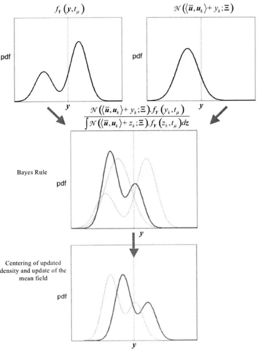
4.4 Update of the stochastic subspace using data and measurements . . . 84
4.4.1 Data and measurements formulation . . . . 84
4.4.2 Update of the stochastic information inside Vs . . . . 85
4.4.3 Expansion of the stochastic subspace VS . . . . 89
5 Application of dynamically orthogonal field equations to random fluid flows 91 5.1 Form ulation . . . . 92
5.2 Derivation of DO Navier-Stokes equations . . . . 94
5.2.1 Stochastic pressure field . . . . 95
5.2.2 Evolution of the mean field ii (x, t; w) . . . . 97
5.2.3 Evolution of the stochastic subspace basis ui (x, t; w) . . . . . 97
5.2.4 Evolution of the stochastic coefficients Y (x, t; w) . . . . 98
5.3 The case of stochastic boundary conditions . . . . 100
5.4 Unstable perturbations for Navier-Stokes equations . . . . 102
5.5 Transfer of energy in Navier-Stokes . . . . 105
5.5.1 Energy exchanges between the DO modes and the mean flow . 106 5.5.2 Energy exchanges between the DO modes . . . . 108
5.5.3 Stochastic energy in Navier-Stokes . . . . 109
5.6 Application I: Lid driven cavity flow with stochastic initial conditions 111 5.6.1 Evolution of a small stochastic perturbation . . . . 117
5.7 Application II: Flow past a circular disk with stochastic initial conditions 122 5.8 Application III: Instabilities in the forced double gyre flow in a basin 134
5.8.1 M odel . . . . 135
5.8.2 An overview of deterministic analysis . . . . 136
5.8.3 Bifurcation analysis of the stochastic response . . . . 137
5.8.4 Stochastic response for larger Reynolds number . . . . 155
6 Finite-size particles in stochastic flows 6.1 Introduction . . . . 6.2 Summary of results for finite-size particles in deterministic flows 159 160 162 162 6.2.1 Reduced order dynamics 6.2.2 Instabilities on the dynamics of finite-size particles . . . . 171
6.2.3 Clustering of finite-size particles . . . . 174
6.3 Dynamics of finite-size particles in stochastic flows . . . . 178
6.3.1 Stochastic velocity field . . . . 178
6.3.2 Markov (diffusion) approximation . . . . 179
6.3.3 Stochastic slow manifold . . . . 184
6.3.4 Stochastic inertial equation . . . . 186
6.3.5 Stochastic source inversion . . . . 189
6.4 Higher order Lagrangian stochastic models . . . . 189
6.5 Clustering due to stochasticity of the flow . . . . 191
6.6 Application: Particles in the double gyre flow . . . . 194
6.6.1 Stochastic slow manifold in the flow . . . . 195
6.6.2 Convergence to the stochastic slow manifold . . . . 197
6.6.3 Validation of stochastic inertial equation . . . . 203
6.6.4 Clustering due to the combined effect of inertial and flow stochas-ticity . . . . 7 Conclusions 7.1 Future directions . . . . 203 209 211 NNW
A DO equations for 3D Navier-Stokes in component wise form A.1 Stochastic pressure field .... ...
A.2 Evolution of the mean field d (x, t; w) . . . . A.3 Evolution of the stochastic subspace basis Xi (x, t; w) . . . . . A.4 Evolution of the stochastic coefficients Y (x, t; w) . . . . B Numerical implementation of 2D DO for Navier-Stokes,
B.1 Initial conditions formulation . . . . B.1.1 Storage of orthonormal basis . . . . B.2 Evolution of stochastic state . . . . B.3 Diagonalization of covariance matrix - Adaptive criteria . . . . B.4 Storage - Plotting . . . . C Normal local stability of general invariant manifolds
C.1 Set-up and definitions . . . . C.2 Normally stable and normally unstable subsets . . . . . C.3 Computing the NILE . . . . C.4 Locating stable and unstable neighborhoods of M(t) C.5 Stability properties of non-neutrally buoyant particles
229 . . . . 230 . . . . 231 . . . 235 . . . . 236 . . . . 239 213 216 218 219 221 223 223 224 224 225 227
List of Figures
2-1 Ellipsoid that contains the main spread ('mass') of the probability mea-sure; defined by the principal directions and the associated eigenvalues of the correlation operator. . . . . 45 3-1 a) The stochastic subspace Vs spanned by fields ui (x, t) that
corre-sponds to important variance. b) The variation of the ui (x, t) inside V, can always be covered by a rotation of the stochastic coefficients
Yi(t;w). ... .. . . . .. . . . . .... .. . . . . .. . . .. 61 4-1 Computational time (sec) for the lid-driven cavity flow described in
Chapter 5, using different number of modes (red curve). The blue line indicates the linear 'best fit' in the log-log plot and it has an inclination equal to 1.986 (2 is the theoretical prediction). . . . . 77
4-2 Decomposition of the stochastic subspace Vs based on the data
sub-space V o.. . . . . . . . . 86
4-3 Update of the probability density function fy (y, t) using data or mea-surem ents. . . . . 88
5-1 Energy exchanges between DO modes and the mean flow in stochas-tic, homogeneous, Navier-Stokes equations. The energy flow from the mean to the modes is characterized by the second order statistics while
variance exchange among the modes is characterized by the third order statistics. . . . . 112
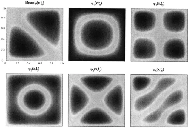
5-3 Initial conditions for the mean and the basis of the stochastic subspace
Vs in terms of the field streamfunction. . . . . 113
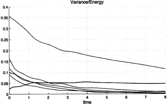
5-4 Evolution of principal variances o? (t), i = 1,..., 5 (blue curves) and mean field energy (red curve) for the flow in a cavity. . . . . 114
5-5 Mean field and basis of the stochastic subspace Vs in terms of the streamfunction and vorticity field; two-dimensional marginals of the five dimensional joint pdf
f
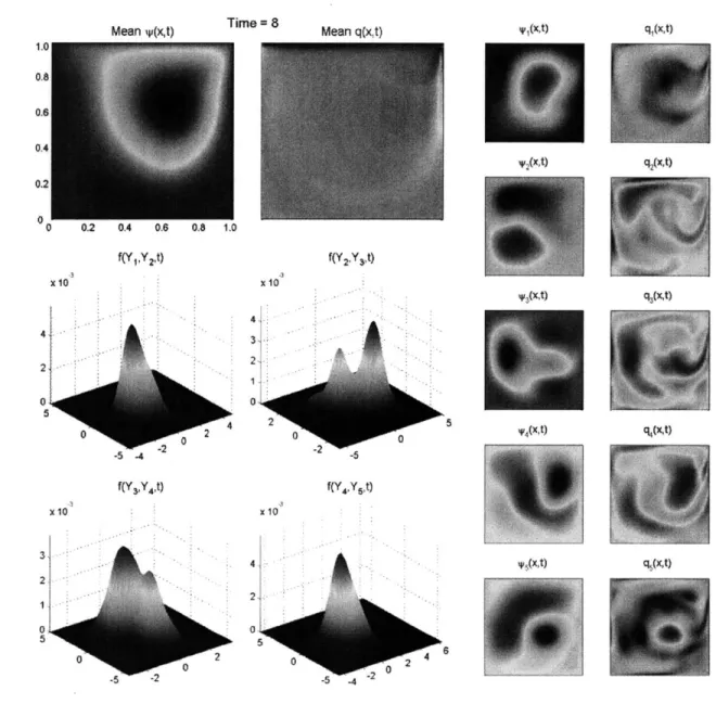
(y, t) at time t = 2. . . . . 1155-6 Mean field and basis of the stochastic subspace Vs in terms of the streamfunction and vorticity field; two-dimensional marginals of the five dimensional joint pdf
f
(y, t) at time t = 8. . . . . 1165-7 Mean velocity field (streamfunction) computed using Monte-Carlo method (250 and 500 samples) and the DO field equations (s = 5 modes) at t = 1 . . . . 117
5-8 Upper plots: mean flow for t = 0.7 in terms of the streamfunction for i) the four modes solution and ii) the five modes solution. Lower plot: the red curves represent the time series for the variances of (t), i = 1, .., 5 of the five-modes solution v (x, t; w) while the blue curves represent the projection of the four modes solution u (x, t; w) to the m odes vi (x, t) . . . . 119
5-9 Upper plots: mean flow for t = 5.98 in terms of the streamfunction for i) the four modes solution and ii) the five modes solution. Lower plot: the red curves represent the time series for the variances of
(t),
i = 1, .., 5 of the five-modes solution v (x, t; w) while the blue curves represent the projection of the four modes solution u (x, t; w) to the m odes vi (x, t). . . . . 1205-10 Mean flow for various stochastic dimensionalities and for t = 1. ... 123
5-11 Mean flow for various stochastic dimensionalities and for t = 2. ... 124
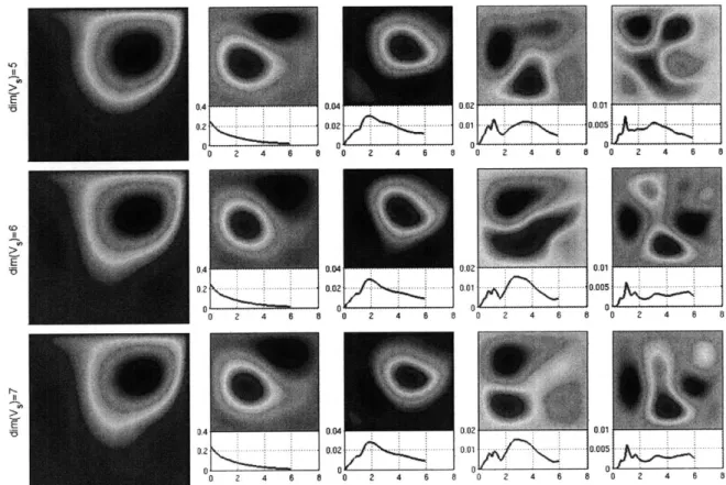
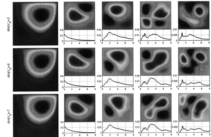
5-13 Left column: mean flow for various stochastic dimensionalities dim (Vs) at t = 2. The four right columns on the right show the four most en-ergetic modes ui (x, t) in terms of their streamfunction as well as their associated variance EW [Y2 (t; w)] as a function of time. . . . . 126 5-14 Left column: mean flow for various stochastic dimensionalities dim (Vs)
at t = 6. The four right columns on the right show the four most en-ergetic modes ui (x, t) in terms of their streamfunction as well as their associated variance EW [Y (t; w)] as a function of time. . . . . 127 5-15 Left column: mean flow for various stochastic dimensionalities dim (Vs)
at t = 8. The four right columns on the right show the four most en-ergetic modes ui (x, t) in terms of their streamfunction as well as their associated variance EW [Y? (t; w)] as a function of time. . . . . 128 5-16 Upper plot: instantaneous error of the solution with respect to the
number of modes used and time. Lower plot: time averaged error with
respect to the number of DO modes. . . . . 129
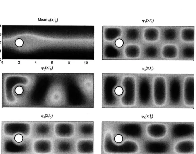
5-17 A typical realization of the flow past a circular disk. . . . . 129 5-18 Initial conditions for the mean and the basis of the stochastic subspace
Vs in terms of the field streamfunction. . . . . 130
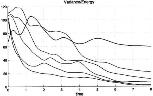
5-19 Evolution of principal variances oi (t), i = 1, ..., 5 (blue curves) and
mean field energy (red curve) for the flow behind a disk. . . . . 131
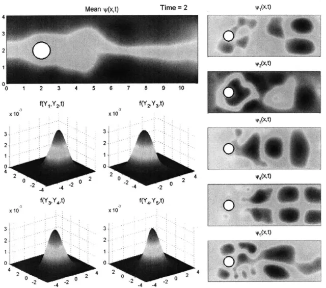
5-20 Mean field and basis of the stochastic subspace Vs in terms of the streamfunction; two-dimensional marginals of the five dimensional joint pdf
f
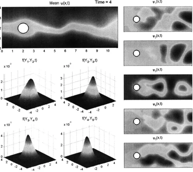
(y, t) at time t = 2. . . . . 132 5-21 Mean field and basis of the stochastic subspace Vs in terms of thestreamfunction; two-dimensional marginals of the five dimensional joint pdf
f
(y, t) at time t = 4. . . . . 133 5-22 Mean velocity field (streamfunction) computed using the DO fieldequations (s = 5) and Monte-Carlo method (500 samples) at t = 1. . 134
5-23 Bifurcation diagram for the QG model with values of the parameters as in Tables 5.1 and 5.2 (from Simonnet and Dijkstra [133]). .. .. . 138
5-24 Spectral behavior of the eigenmodes involved into the various bifurca-tions of the anitsymmetric branch for the barotropic QG model (from Simonnet and Dijkstra [133]). . . . . 139
5-25 Stochastic responce of the QG model for Re = 25. The left top plot shows the mean flow in terms of the vorticity (colormap) and the streamlines (black solid curves). The right-top plot indicates the en-ergy of the mean flow (red curve) and the variance of the stochastic mode. The bottom plot indicates the first DO mode together with the pdf for the stochastic coefficient. . . . . 140
5-26 Stochastic responce of the QG system for Re = 35 after the system has reached steady state statistics. . . . . 141
5-27 Oscillation of the DO mode during convergence to the steady state attractor for Re = 35 . . . . 142 5-28 Addition of an extra mode at the time instant where the existing mode
exceeds the predefined variance (Flow Re = 38). . . . . 144
5-29 Mode removal due to very low variance (Flow Re = 38). . . . . 145 5-30 The variance of the stochastic perturbation becomes comparable with
the energy of the mean flow. At this point mutual interactions between the mean flow and the perturbation begin to occur. . . . . 146
5-31 Steady state regime for Re = 38. Note that the perturbation retains its symmetric character even though the variance of the mode is com-parable with energy of the mean flow. . . . . 147
5-32 Stochastic response for Re = 40. Note that the first mode has sym-metric spatial properties which are accompanied by symsym-metric pdf while the second mode has antisymmetric spatial properties with non-sym m etric pdf. . . . . 148
5-33 Initial stage of motion for Re = 55. . . . . 149 5-34 As time evolves more modes have to be added in order to achieve the
5-35 Convergence to a deterministic attractor after a transient stochastic regim e for Re = 65. . . . . 151
5-36 Response for Re = 85. In this case the convergence to the deterministic attractor occurs earlier with the initial stochastic regime being much sorter in tim e. . . . 152 5-37 Convergence to a deterministic attractor for Re =100. . . . 153 5-38 Stochastic attractor after a temporal convergence to deterministic
dy-namics (Re = 200). . . . 154 5-39 Summary of the stochastic analysis for the double gyre flow over various
Reynolds numbers. . . . . 154
5-40 Initial regime of the stochastic response for Re = 104. . . . . 156 5-41 The modes added are localized around the boundary of the formed
gyres of the mean flow. . . . 156 5-42 After the mean flow energy exceeds a certain limit an instability breaks
the symmetry of the third mode as it is shown in the corresponding pdf plot. . . . . 157 5-43 The instabilitiy shown in the previous figure is the starting point for
the non-Gaussian statistics shown here. . . . . 158
6-1 (a) The geometry of the domain Do (b) The attracting set of fixed points Mo; each point p in MO has a n-dimensional stable manifold fo(p) (unperturbed stable fiber at p) satisfying (x,
#)
= const. . . .. 167 6-2 (a) The geometry of the slow manifold M, (b) A trajectory intersectinga stable fiber
f,
(p) converges to the trajectory through the fiber base point p . . . . . 1686-3 Sudden changes in the velocity field delay convergence to the slow m anifold . . . . 170
6-4 Particle velocity (blue solid curve) attracted by a concentrated layer of probability, a stochastic slow manifold. The red solid curve denotes the mean of the manifold and the dotted curves define the local spread
of probability around the mean. . . . . 185
6-5 Clustering manifold is independent from the flow direction. . . . . 192 6-6 Stochastic double gyre for the illustration of the inertial particles
mo-tion; Re = 25 (See chapter 5 for details). . . . . 196 6-7 Mean value of the stochastic slow manifold governing the motion of
inertial particles for the double gyre stochastic flow. . . . . 197
6-8 Variance of the stochastic slow manifold descrbing of motion inertial particles for t = 100.0 and t = 100.5. . . . . 198 6-9 Variance of the stochastic slow manifold descrbing of motion inertial
particles for t = 101.0 and t = 101.5. . . . . 199 6-10 (a) Rapid convergence to the stochastic slow manifold during the initial
phase of motion. The colormap denotes the local variance of the slow manifold -, (x, t) . The vertical coordinate shows the distance of the
stochastic dynamics from the mean slow manifold. (b) x- component of the particle velocity, resolved according to Maxey-Riley equation for a particular flow realization (blue solid curve). The red lines indicate the local spread of probability around the mean slow manifold at the particle's location. (c) same as (b) but now the distance from the slow m anifold is shown. . . . . 201
6-11 Same as 6-10 but for a later time instant. . . . . 202
6-12 Comparison of stochastic inertial equation (6.40) and direct Monte-Carlo simulation for t = 100, 101, 102. . . . . 204 6-13 Same as Figure 6-12 for t = 103, 104. . . . . 205 6-14 Concentration field for finite size particles (heavy particles) for two
different time instants. The blue lines indicate streamlines for the mean flow. The red lines indicate clustering manifolds for the stochastic flow field . . . . 207
B-1 Computational algorithm for the adaptive DO equations. . . . .2
C-1 Trajectories jump away from M(t) over the unstable subset M,(t), but return to M(t) over the stable subset M,8(t). The figure assumes that
M(t) is a normally hyperbolic attracting manifold, in which case the
jumping trajectory keeps approaching the same underlying trajectory on M(t) by the invariant foliation of the stable manifold Ws(M(t)). 232
C-2 The operator I", Ftt +(p) DFt+sNM(t) maps vectors in the normal space NpM(t) to vectors in the normal space NFt+,(P)M(t + s). The NILE
-(p; t) is the exponential rate at which the norm of the above operator
grows in the limit of infinitesimally small s. Therefore, a-(p; t) measures the exponential rate at which the normal component of vectors normal to the manifold M(t) grows over very short times. (The time T is arbitrary within the interval [t, t
+
s].) . . . . 233 C-3 The manifold M(t) as a local graph over the x variables. . . . . 235 226List of Tables
5.1 Reference values of parameters in the barotropic QG model
(dimen-sional). . . . . 136
5.2 Reference values of parameters in the barotropic QG model (non-dim ensional). . . . . 136
6.1 Reference values of parameters in the barotropic QG model used for the study of finite-size particles (dimensional). . . . . 195
Chapter 1
Introduction
Dynamical systems play a central role in applications of mathematics to natural and engineering sciences. However, dynamical systems governing real processes always contain some elements characterized by uncertainty or stochasticity. Uncertainties may arise in the system parameters, the boundary and initial conditions, and also in the 'external forcing' processes. Also, many problems are treated through the stochastic framework due to the incomplete or partial understanding of the govern-ing physical laws. In all of the above cases the existence of random perturbations, combined with the complex dynamical mechanisms of the system itself can often lead to a rapid growth of the uncertainty in the dynamics and state of the system. Such rapid growth can distribute the uncertainties to a broadband spectrum of scales both in space and time, making the system state particularly complex.
In the past decades an increasing number of problems in continuum theory have been treated using stochastic dynamical theories. Such problems are mainly described by stochastic partial differential equations (SPDEs) and they arise in a number of ar-eas including fluid mechanics, elasticity, and wave theory, describing phenomena such
as turbulence, random vibrations, flow through porous media, and wave propagation through random media. This is but a partial listing of applications and it is clear that almost any phenomenon described by a field equation has an important subclass of problems that may profitably be treated from a stochastic point of view.
turbulent flows. In turbulence the spatial and temporal dependence of the instan-taneous values of the fluid dynamics fields have a very complex nature. Moreover, if turbulent flow is setup repeatedly under the same conditions, the exact values of these fields will be different each time. However, even though the details of the flow maybe different over various runs, it has been observed that their statistical prop-erties remain similar, or at least coherent over certain finite-time and space scales. These observations lead to the natural conjecture that statistical modeling or statis-tical averaging over appropriate spatial and temporal scales maybe more efficient for the description of these phenomena.
In this work, we develop a new methodology for the representation and evolution of the complete probabilistic response of infinite-dimensional, random, dynamical systems. More specifically, we derive an exact, closed set of evolution equations for general nonlinear continuous stochastic fields described by a Stochastic Partial Differ-ential Equation (SPDE). By hypothetizing a decomposition of the solution field into a mean and stochastic dynamical component that are both time and space dependent, we derive a system of field equations consisting of a Partial Differential Equation (PDE) for the mean field, a family of PDEs for the orthonormal basis that describe the stochastic subspace where the stochasticity 'lives' as well as a system of Stochastic Differential Equations that defines how the stochasticity evolves in the time varying stochastic subspace. These new Dynamically Orthogonal (DO) evolution equations are derived directly from the original SPDE, using nothing more than a dynamically orthogonal condition on the representation of the solution. This condition is the 'key' to overcome the redundancy issues of the full representation used while it does not restrict its generic features. Therefore, we do not assume an a priori representation neither for the stochastic coefficients, nor for the spatial structure of the solution; all this information is obtained directly by the system equations, boundary and initial
conditions. If additional restrictions are assumed on the form of the representation, we recover both the Proper-Orthogonal-Decomposition (POD) equations and the gen-eralized Polynomial-Chaos (PC) equations. For the efficient treatment of the strongly transient character on the systems described above, we derive adaptive criteria for
the variation of the stochastic dimensionality that characterizes the system response. Those criteria follow directly from the dynamical equations describing the system. We also describe how information obtained from full-field data inputs can be merged with the numerically evolved stochastic fields within the context of DO equations.
Since the basis of the stochastic subspace is evolving according to the system
SPDE, fewer modes are needed to capture most of the stochastic energy relative to the classic POD method that fixes the form of the basis a priori, especially for the case of transient responses. On the other hand, since the stochasticity inside the dynamically varying stochastic subspace is described by a reduced-order, exact set of SDEs, we avoid the large computational cost of PC methods to capture non-Gaussian behavior. Therefore, by allowing the stochastic subspace to change we obtain a bet-ter understanding of the physics of the problem over different dynamical regimes without having the well known cost or divergence issues resulted from irrelevant
rep-resentations of spatial (in POD method) or stochastic structure (in PC method). We illustrate and validate this novel technique by solving the 2D Navier-Stokes equations in various geometries and compare with direct Monte Carlo simulations. We also apply the derived framework for the study of the statistical responses of an idealized 'double gyre' model, which has elements of ocean, atmospheric and climate instability behaviors.
Finally, we use our new stochastic description for flow fields to study the mo-tion of inertial particles in flows with uncertainties. Inertial or finite-size particles in fluid flows are commonly encountered in nature (e.g., contaminant dispersion in the atmosphere) as well as in technological applications (e.g., chemical systems in-volving particulate reactant mixing) and as it has been observed both numerically and experimentally, their dynamics can differ markedly from infinitesimal particle dynamics. Here we use recent results from stochastic singular perturbation theory
in combination with the DO representation of the random flow, in order to derive a reduced order inertial equation that will describe efficiently the stochastic dynamics of inertial particles in arbitrary random flows.
1.1
Preview of chapters
This thesis is organized as follows. In Chapter 2 we give the necessary notation and summarize basic properties for random fields. We present in detail a generalized form of the Karhunen Loeve expansion, which is a fundamental tool for the reduction of the stochastic dimensionality that characterizes a given problem. We also present a geometrical interpretation of its properties and we illustrate how it can be used for the efficient time and space dependent representation of random fields that characterize fluid motion and have a priori properties such as non-divergence.
Chapter 3 is the central theoretical part of the thesis. Here we derive an exact, closed set of evolution equations for general continuous stochastic fields described by a Stochastic Partial Differential Equation (SPDE). The derivation is based on a novel condition, the dynamical orthogonality, on the representation of the solution, which as we prove, it comes naturally without imposing any constraints on the form of the response. Based on this condition we derive a system of field equations consisting of a Partial Differential Equation (PDE) for the mean field, a family of PDEs for the or-thonormal basis that describe the stochastic subspace as well as a system of Stochastic Differential Equations that defines how the stochasticity evolves in the time varying stochastic subspace. We also prove that under additional restrictions on the form of the representation, the DO field equations reproduce both the Proper-Orthogonal-Decomposition equations and the generalized Polynomial-Chaos equations; thus the new methodology unifies these two approaches.
The scope of Chapter 4 is to develop adaptive criteria for the dimensionality of the stochastic subspace in the context of the dynamically orthogonal field equations. We present adaptive criteria for the contraction and expansion of the stochastic subspace and we also illustrate how the new stochastic dimensions should be chosen (when the stochastic subspace should be expanded) according to stability arguments. These
criteria are based on the current stochastic response of the system and they use a priori hypotheses on the spectrum of the orthogonal complement of the stochastic subspace. Note that we restrict ourselves to the 'internal' adaptation, i.e. we assume that the
realizations of the full fields resulting from our simulations are the new information used in the adaptation. This is different from adaptation to external irregular data.
In Chapter 5 we apply the Dynamically Orthogonal field equations to the case of two dimensional random flows described by Navier-Stokes equations with and with-out the Coriolis force due to a rotating reference frame. In the first two sections we formulate the problem and we derive closed, evolution equations for the mean field, the scalar stochastic coefficients, and the DO modes. We also discuss the case
of stochastic boundary conditions and we prove that this family of problems can always be reformulated as problems with deterministic boundary conditions and suit-able forcing. Subsequently, we present numerical results for specific geometries and forcing configurations and we will examine convergence properties of the proposed methodology. In the last section of the chapter we consider an idealized model for the description of the temporal variability of the wind-driven, vertically averaged, ocean circulation. The aim of this section is to study the stochastic response of this model for different forcing parameters and Reynolds regimes. Through the developed stochastic framework we shall prove that in the unstable regimes, as those are pre-dicted by the deterministic theory, the system converges to a stochastic steady state response which is characterized by finite variance that is smaller than the energy of the mean flow. For larger Reynolds or forcing amplitude, we find that this variance may become comparable with the energy of the mean flow giving rise to periodic or even chaotic responses.
In Chapter 6 we apply our theoretical and numerical results derived for the
de-scription of stochastic flows in order to study the motion of finite-size particles in flows with uncertainty. Specifically, we examine the coupled effects due to inertia and flow stochasticity. In the first part of the chapter we summarize theoretical results for particles in deterministic flows. Subsequently we present results for the stochastic case. Specifically, we prove that the velocity of finite-size particles is governed by a
stochastic slow manifold, a 'layer' of probability around the deterministic slow man-ifold derived previously for deterministic flows. Based on a stochastic reduction on this manifold we derive a stochastic inertial equation that governs the motion of
par-ticles and which includes new terms expressing the coupled effect of parpar-ticles inertia and stochasticity. In the second part of the chapter we first illustrate numerically the convergence of the particles stochastic velocity to the stochastic slow manifold. We validate the derived inertial equation for a specific example and we analyze the
cou-pled effects of particles inertia and flow stochasticity on the preferential concentration of particles. In Chapter 7 we summarize the contributions of this work.
Chapter 2
Representations of stochastic fields
Abstract
The primary purpose of this chapter is to give the necessary notation and summa-rize basic properties for random fields. In the first section we give the definition of a stochastic phenomenon. Subsequently we provide with a brief description of the mathematical tools used for the representation of stochastic fields such as proba-bility density functions, moments, and the characteristic functional. We also prove that those different descriptions are equivalent. The next section refers to Karhunen Loeve expansion, which is a fundamental tool for the reduction of the stochastic di-mensionality that characterizes a given problem. We give a geometrical interpretation of its properties and we illustrate how it can be used for the efficient representation of random fields that characterize fluid motion and have a priori properties such
non-divergencess.
2.1
Introduction
Many problems arising in nature and technology can be profitably treated from a
stochastic point of view. A common characteristic for these problems is the presence of uncertainties in the system parameters, and disordered or random perturbations in the dynamical variables that describe the system state. Also, many problems are treated
through the stochastic framework due to the incomplete or partial understanding of the governing physical laws or simply because the stochastic approach is the most efficient way of doing computations (e.g. turbulence). In all of the above cases the existence of random perturbations, combined with the nonlinearities of the system often leads to their rapid growth which causes distribution of energy to a broadband spectrum of scales both in space and time, making the system state particularly complex.
Probably the most characteristic representative from this family of problems are turbulent flows. In turbulence the spatial and temporal dependence of the instan-taneous values of the fluid dynamics fields have a very complex nature. Moreover, if turbulent flow is setup repeatedly under the same conditions, the exact values of
these fields will be different each time (see e.g. Monin and Yaglom [102]). However, even though the details of the flow maybe different over various runs, it has been
observed that their statistical properties remain similar leading to the natural con-jecture that statistical modeling or statistical averaging over appropriate spatial and temporal scales ('spectral windows', [105]) maybe more efficient for the description of these phenomena.
The primary purpose of this chapter is to introduce the mathematical tools used for the description of random fields. Before we proceed to the definition of a random or stochastic fields we shall first give a more formal definition of what we mean by a random or stochastic phenomenon. We consider a sequence of runs for the same experiment flW (where w denotes an arbitrary realization) that describe a given
phe-nomenon, IfWl, I 2 ... , UlWn ...and the corresponding sequence of results R'I, RtW2,...,
RWn, .... In many cases the following relation holds for the outcomes of the various
runs
d (Ri, Rw) <e for all i, j (2.1)
where d is a suitable metric (i.e. distance, see e.g. [104)) and s, is a predefined level of tolerance. The above behavior leads to the commonly expected result that different runs of the same experiment leads to close results. From the above discussion we
have the following definition [7]
Definition 1 A phenomenon will be called deterministic if, for every experiment UW that is associated with it, any sequence of experimental runs li satisfies eq. (2.1) with sufficiently small ed,. In contrary if relation (2.1) is not valid for one or more experiments then the phenomenon will be called nondeterministic.
Therefore, the definition of a deterministic or nondeterminisitc phenomenon de-pends strongly on the tolerance level E, as well as on the metric d. Even though an experiment associated with a nondeterministic phenomenon presents important variability in terms of results, this picture may change if we consider mean values of the outcomes for a large sequence of runs, e.g. the ensemble mean
R&I + RW2 + ... + R&N
RW±R 2 +=W
N
Then, it is possible to have sufficiently close mean values RN over different sequences of runs {Hw}% for the same experiment UJ
d
(R<,
R. <e, for any large experimental sequences {1}i ,{ir}.
In this case the experiment is said to present statistical stability [163]. Using this concept we proceed to the definition of a stochastic or random phenomenon ([163],
[7])
Definition 2 A nondeterministic phenomenon will be called stochastic or random if the results of any associated experiment with it UlW, present statistical stability.
We shall now define the appropriate tools for the mathematical modeling of
stochastic phenomena. In the theoretical modeling of random phenomena the
ba-sic role is played by the probability space (Q, EQ, P) . The set Q, which we call sample space, includes all the possible outcomes of a given phenomenon. EQ is a o-algebra of subsets of Q [67], i.e. a set of subsets that has the following properties i) Q E EQ,
ii) if A E EQ then its complement is also in EQ, iii) Every countable union of the
ele-ments of Eg, i.e. every Ai E EQ, is in EQ. Based on these two concepts we define the probability measure Pn as a set function from EQ to the interval [0, 1] which satisfies the three axioms of probability ([67], [135]).
For every physical realization w E Q, we may correspond a quantity u (w) E U, where U is a suitable set (e.g. a subset of R, a set of functions, or a set of fields). Therefore the abstract set Q contains all the possible physical realizations of the phenomenon, while U contains their corresponding mathematical description. For example, in the case of a random flow, w E Q will represent a particular physical realization of the flow, while u (w) will represent a specific mathematical quantity associated with the flow e.g. the velocity field. This leads to the concept of a stochastic process or stochastic field. Specificallywe have the following formal definition
Definition 3 A stochastic field is a function u (x, t; w) = {uj (x, t; w)},1 E Rm,
x E D c R", t E T, w E Q, defined on a sample space Q, a spatial domain D, and a time interval T, such that, for every x E D C R" I t E T and every real vector r E R' the set {w :u (x,t;w) <r.,
j
= 1, ..., m} is inside EQ.Having a stochastic field, there are at least three different kinds of methods to obtain statistically averaged properties. They are space averages, time averages, and ensemble averages. The usefulness of space averages is limited to fields that are statistically homogeneous or at least approximately homogeneous over scales larger than those of the random features. Similarly, time averages are useful only if the stochastic field is in effect statistically stationary over time scales much larger than the time scale of the stochastic properties. In both of the above cases averaging over the appropriate 'spectral window' (i.e. range of spatial and temporal scales, [105])
may significantly simplify the problem. The third type of average, ensemble averages, does not assume anything on the statistical characteristics of the random field (e.g.
homogeneity or stationarity) and for this reason it is the most versatile. In what follows every averaged quantity will be in the sense of ensemble average and will be
denoted as
E[u.(w)] = U(Wi) + U W( 2) + ... + U (WN)
N--+oo N
where wi E Q are specific realizations. In the following sections we will present the essential tools used for the analysis and description of stochastic fields in terms of their statistical and physical properties.
2.2
The family of probability density functions
In this section we will give the definitions of probability density functions and also
present the essential notation that will be used in the rest of the thesis. Given a stochastic vector field u (x, t; w) defined as above, we have for every collection of spatial positions xi,x 2, ... , XN and time instants t1, t2, ---, tN the joint probability
distribution function
FU(x1,t1),--,u(XNtN) (U1, ---, UN) = :
u
u (xi, ti; w) < u1n
... flU (XN, tN; w) < UNwhere each inequality is meant in the component-wise sense, i.e. uj (x1, ti; w) <
u1 ,
j
= 1, ..., m. This family (the term 'family; follows from the fact that the jointdistribution function is defined for arbitrary combinations of time instants and space locations) will always satisfy the Kolmogorov compatibility conditions [67
1) the symmetry condition: if {i1, i2, ---, IN} is a permutation of numbers 1, 2, ..., N
then for arbitrary N > 1
Fu(x11),---,xNN) (U1, -- , UN) = F .U(xiN tiN 1, ''', UiN)
2) the consistency condition: for M < N we have
lim Fu(x1,ti),...,u(x,tM),---u(xNtN) (U1, ---, UN) = Fu(xi,ti),-,u(xmAt) (U1, ..., u M) j>M
field u (x, t; w). Therefore a complete statistical characterization of a random field involves the characterization of the full family of probability distribution functions.
In the special case where Fu(x1,t1),.,U(XN,tN) (U1, ---, UN) is differentiable with
re-spect to its arguments (U1, ... , UN) for every collection of spatial locations and time
instants we can alternatively use the probability density function (see e.g. [109])
fu(x1,t1),.-U(XN,tN) (U1, ... , UN) O-N Fu(x1,ti),--,U(xN,tN) (U1, ... UN)
aOUl... aUN
where
a- am
8. &U& 2 "
-au all18U2
-.
-a-lm'
Note that for the special case of scalar fields described by the probability distribution function
FU(x1,.1),---,U(XN,tN) (U1, ... UN) = [ W-u (xi, ti; W)
<u
i O ... fu(XN,
tN; W) < UN} ,the definition of the probability density function has the simpler form
fU(x1,t1),...,u(xN,tN) (U1, --- UN) = u UN Fu(x1,tl),...,U(XN,tN) (U1, -- UN)
-In the general case the family of probability density functions satisfies the following conditions
1) the non-negativity condition
fu(x1,t1),---,U(xNstN) (U1, ... UN) > 0
2) the normalization property
J
fu(x1,t1),..,(xNtN) (U1, ... UN) dul...duN 13) the marginal property
J fu(x1,i),...u(xNtN) (Ui, ... , UN) duM+1...dUN = fu(x1,t1),.,u(XM,tM) (U1, ... , UM)
R(N-M).m
For the fields that we will consider in the present work we will assume that the
probability distribution functions of every order (i.e. for any number of joint time instants and space locations - e.g. second order are the joint probability density functions involving two time instants and space locations) exist and they are also differentiable. In this case an alternative tool for the description of a stochastic field is given by the family of characteristic functions defined as
Ou(x1,t1),.,u(XN,tN) (6, -- , N) [fu(x1,ti),..,u(XN,tN) ( '''
N
=
"
[expiu
3
(xy,
t; W)U
) (j=1where F denotes the Fourier transform. The family of characteristic functions possess the following properties
1) the normalization property
Ou(x1it1),---,U(XNtN) (07 ... 1
2) the boundness property
4Ou(x1,ti),---,U(XN,tN)
(61...
,
&)
C'1
for
all
((1, ---, N) E RN.m3) the symmetry property
wU(x1,ti),...,u( xNctN)
(
u1 ,N(x,ti),...,u(xNtN) c(
6
1 --- ~ where * denotes the complex-conjucate.4) the marginal property
4u(x1,t1),---,u(xN,tN) 1, ---, M, 0, '0) U(X1,t1) ,...,U(XMtM) (61 , - 7M)
-5) positive definiteness: for every vector c C ZM (with c* denoting the complex conjugate of c) we have
M M
u(x 1,t1)-.-,u(XNtN) (61i - '1, ---, CMi - 6Mj) cic 0
j=1 i=1
for any collection of vectors Rm E 6ij, i, j = 1, ... , M.
2.3
The moment system
The next important concept for the description of stochastic or random fields is the statistical moments. For a stochastic vector field u (x, t; w) defined as above, we have the statistical moments of the first order
ii (x, t) = E' [u (x, t; w)] = Jufu(xt) (u) du E Rm R
It is often necessary to investigate the joint behavior of the field at two different
spatiotemporal locations. For this case we define the correlation operator (or second moment)
Ru(xl,t1;w)u(x 2,t2;W)Ew [u (x1, t1; W) u (x2, t2; W)T
= uJUTUfu(x1,ti)u(x2,t2) (ui, u2)
duidu
2 ER"'.
An alternative definition is given by the correlation coefficient which is a normalized version of the correlation operator.
In many occasions it is often more convenient to work with central moments. The
second moment)
Cu(x1,ti;W)u(x2,t2;w)=Ew [(U (x1, ti; W) - t (xI, ti; O)) (u (x2, t2; W) - ii (x2, t2; w))T
Since, for what will follow we will make extensive use of the above operator at the same time instants ti = t2 but at different locations we will use the following notation
for the spatial covariance
Cu(-,tw)u(.,t;w) (x, y) = Cu(x,tw),u(y,t;W)
=E' [(u (x, t; w) - ii (x, t; w)) (u (y, t; w) - i (y, t; w))T]
The above quantities define the second-order statistical characteristics for the field u (x, t; w). Their knowledge is sufficient for a complete stochastic description for the
case of Gaussian fields (see e.g. [1093). However, for the general case, the com-plete family of moments is required. Specifically, a comcom-plete stochastic description of
u (x, t; w) requires the knowledge of all moments of order r
E" [ujl (X1, ti; W) Uj, (X2, t2; W) --- Ujr (xr, tr; W)]
= UjUj 2 ... UjrfU(Xi,ti)U(X2,t2),...,U(Xr,tr) (ui, U2, ..., Ur) duidU2 ...dur Rm.r
for every combination of spatial locations x1, x2, ... , Xr, time instants ti, t2, ..., tr,
in-dices j = (jiJ2, ---,jr) , (with jE E {1, ..., m}) and r = 1, 2 . Note that in the above
definition u31 denotes the
ji
component of ui and so on.2.3.1
Connection with the family of characteristic functions
We saw previously that the system of statistical moments is connected to the family of probability density functions. This is also true for the family of characteristic
functions. Specifically, we can express any statistical moment as (see e.g. [136])
E"' [U, (x1, t1; w) Uj, (x2, t2; w) ---ZUj (xr, t; w)
1r _________...___ ,U(X 1,t1),.U(XN,tN) (1 - N N)- =0
where (1j is the ji component of the vector (1 and so on. The above property is a direct consequence of the definition of the characteristic function through the Fourier transform of the corresponding density. Hence we have presented three different approaches for the complete probabilistic description of a stochastic field and we have also recalled their connection. For all the presented approaches the definition is given in terms of a system that includes all possible combinations of spatial locations and time instants. In the next section we describe an infinite dimensional tool that captures the complete probabilistic information in a singe functional.
2.4
The characteristic functional
We saw that the tools presented so far follow a bottom-up approach in the sense that we define the global statistical behavior through the definition of finite-dimensional joint statistical quantities such as probability density functions at various locations and time instants or moments associated with them. A top-down approach will involve the consideration of an infinite dimensional quantity that will be able to re-produce all the finite-dimensional information. Such a quantity is the characteristic functional defined directly in terms of the full probability measure '. More
specifi-cally, we have the following definition ([1361, [102], [120])
R, t E T, w E Q, the characteristic functional is defined as
1u [9] = E' exp i Ju (x, t; w)T 9 (x, t) dtdx
=
J
exp( if/u (x, t; w)T q (x, t) dtdxdP (w)
0 (Rm T
where 9 (x, t) E R', x E D C R", t E T, is an arbitrary field.
Therefore, we see that the characteristic functional is a generalization of the family of characteristic functions and therefore it has the same properties i.e.
1) the normalization property
u [0] = 1
2) the boundness property
1u
[0]1 <
1 for all
O3) the symmetry property
4u [0] = <DPU [-6)
4) positive definiteness: for every vector c E ZM (with c* denoting the complex conjugate of c) we have
M M
ZZ u i - Oj cic > 0O j=1 i=1
for arbitrary fields 62 i = 1, ..., M. As mentioned at the beginning, the characteristic
functional contains the full probabilistic information. In fact, through the
character-istic functional we can derive the complete system of moments, as well as the family of characteristic functions and through them the corresponding family of probability density functions.
2.4.1
Determination of the moments system
We shall now illustrate how the characteristic functional can be used to derive
ex-pressions for the moment system. By considering the first Frechet derivative (see e.g. [26]) of the characteristic functional we have
__u Qu [6+sso] - Qu [9] ] J [0; p] = lim 0 s-+o s +E
exp
i
u (x,
t; w)T[9
(x,
t)+
s~p (x,
t)] dtdx
dRm Tf - S=o = iE'ju
(x, t; w)T W (x, t) dtdx expi
u (x, t; w)T 0 (x, t) dtdx Rm T Rm TConsidering the above expression for 0 = 0 we obtain
6(U
[0;
V]
=iE'
u
(x, t; w)T ((x, t) dtdx
LRm T .
Setting 95 (x, t) = 6 (x - xo) 6 (t - to) 6
jk = 6k,xo,to we obtain
6 u
C [0;
okxo,to
iEw [Uk (xO, to; w)] thus1
64UE' [Uk (xo, to; w)] = - 60 [0; 6k,xo,t].
where 6
jk is the Kronecker delta and 6 (t - to) is the Dirac delta function. Depend-ing on the smoothness of the characteristic functional we may consider higher order Frechet derivatives in order to obtain higher order moments. Specifically, we have
62u [0; I, p21 =
= i2E