The Economic Stimulus Payments of 2008
and the aggregate demand for consumption
The MIT Faculty has made this article openly available. Please share
how this access benefits you. Your story matters.
Citation Broda, Christian, and Jonathan A. Parker. “The Economic Stimulus
Payments of 2008 and the Aggregate Demand for Consumption.” Journal of Monetary Economics 68 (December 2014): S20–36.
As Published http://dx.doi.org/10.1016/j.jmoneco.2014.09.002
Publisher Elsevier
Version Author's final manuscript
Citable link http://hdl.handle.net/1721.1/99114
Terms of Use Creative Commons Attribution-Noncommercial-Share Alike
The Economic Stimulus Payments of 2008 and the
Aggregate Demand for Consumption
Christian Broda
Duquesne Capital Management Jonathan A. Parker1*
MIT and NBER
Abstract: Households in the Nielsen Consumer Panel were surveyed about their 2008 Economic
Stimulus Payment. In estimates identified by the randomized timing of disbursement, the average household’s spending rose by ten percent the week it received a Payment and remained high cumulating to 1.5–3.8 percent of spending over three months. These estimates imply partial-equilibrium increases in aggregate demand of 1.3 percent of consumption in the second quarter of 2008 and 0.6 percent in the third. Spending is concentrated among households with low wealth or low past income; a household’s spending did not increase significantly when it learned about its Payment.
Keywords: consumption smoothing, fiscal stimulus, tax policy, consumer demand
JEL classification: E21, E62, D12, D91
1
Address for correspondence: Sloan School of Management, MIT, 100 Main Street, E62-642, Cambridge, MA 02142-1347, 617-253-7218. E-mail: [email protected]. Homepage: http://japarker.scripts.mit.edu/
*
We thank the Sloan School of Management at MIT, the Kellogg School of Management at Northwestern
University, the Initiative for Global Markets at the University of Chicago, and the Zell Center at the Kellogg School of Management for funding for the survey and data. Parker thanks the Laboratory for Applied Economics and Policy at Harvard for funding. For helpful comments on our research, we thank: Jordi Gali, Daniel Green, Greg Kaplan, Ricardo Reis, Sam Schulhofer-Wohl, Nicholas Souleles, anonymous referees on our grant application and at the JME, and participants in numerous seminars and conferences. We would also like to thank Ed Grove, Matt Knain and Molly Hagen at ACNielsen. All results are calculated based on data from the Nielsen Company (US), LLC and provided by the Marketing Data Center at The University of Chicago Booth School of Business. This paper updates and replaces the earlier analysis in Broda and Parker (2008).
1
1. Introduction
The US government passed the Economic Stimulus Act of 2008 in February 2008 in response to the recession that started in December 2007. The main part of Act was a $100-billion program of Economic Stimulus Payments (ESPs) designed to raise consumer demand. The ESPs averaged $900 and were disbursed to US taxpayers in the spring and summer of 2008. Around the time of the stimulus program, measured aggregate consumption is relatively smooth while measured disposable income rises and falls sharply with the disbursement of the Payments, providing “no evidence that the stimulus has had any impact in raising consumption” (Taylor, 2010; see also Feldstein, 2008). On the other hand, previous research finds significant increases in expenditures in response to predictable, predetermined and plausibly-exogenous changes in household-level income.2 Most relevant, Johnson, Parker, and Souleles (2006), Agarwal, Lui, and Souleles (2007), and Johnson, Parker, and Souleles (2009) all find significant spending responses to the receipt of previous Federal tax rebates.3
This paper measures the spending responses of households to the Economic Stimulus Payments of 2008 and quantifies the partial-equilibrium increase in aggregate demand for consumer goods and services caused by the Payments so as to provide quantitative discipline for model-based inferences about the general-equilibrium efficacy of such tax-based stimulus policies. The effect of the receipt of the ESPs of 2008 on the demand for consumption is estimated by first measuring changes in the timing of household spending caused by differences in the timing of the receipt of ESPs, and then aggregating these changes using the temporal distribution of ESPs as reported by the U.S. Treasury and several different extrapolations from the observed goods to a broader measure of spending. ‘Receipt’ is emphasized because our main analysis measures only changes in spending correlated with the date of receipt, so does not include for example changes in spending on the date of announcement. ‘Demand’ is emphasized because the calculation is partial equilibrium and omits any multiplier effects or crowding-out from the policy.
To measure the spending effects of the ESPs, we conducted a multi-wave survey of roughly 60,000 households in Nielsen’s consumer panel (NCP, formerly Homescan consumer
2
See for example Jonathan A. Parker (1999), Nicholas S. Souleles (1999, 2002), and Chang-Tai Hsieh (2003), or the reviews of Deaton (1992), Browning and Lusardi (1996), and Jappelli and Pistaferri (2010).
3
And households when surveyed about what they would do or have done with tax rebates report spending a significant fraction (Shapiro and Slemrod, 1995 and 2003, and Coronado, Lupton, and Sheiner, 2006).
2
panel) during the spring and summer of 2008. The NCP contains annual information on household demographics and income, and weekly information on spending on a set of household goods. Participating households are given barcode scanners which they use to report spending on trips to purchase households goods and to answer occasional surveys designed by Nielsen and typically used to study the efficacy of marketing campaigns. Our supplemental survey, designed in conjunction with Nielsen, uses this existing survey technology to collect information on the date of arrival of the first Economic Stimulus Payment received by each household, as well as its amount, whether it arrived by check or direct deposit, and when the household learned about the Payment. In addition, this survey contains several additional questions useful for our analysis, such as about expectations, access to liquidity and the amount of the ESP spent on NCP and non-NCP items. The resulting dataset has several advantages relative to those used in previous research: the sample is larger, spending is observed weekly, and the ESP information is collected with a short recall window; the main disadvantage is the limited set of goods covered.
We identify the change in spending caused by the receipt of an ESP at the household level following the Johnson, Parker, and Souleles (2006) methodology using the fact that the law randomized the disbursement of ESPs over time. Because it was not administratively possible for the IRS to mail all checks or letters accompanying direct deposits at once, Payments were mailed out to households during a nine-week period between mid-May and the end of July, or deposited into households’ accounts in one of the first three weeks of May. Among mailed checks and among deposited funds, the particular week in which the funds were disbursed depended on the second-to-last digit of the taxpayer's Social Security number, a number that is effectively randomly assigned.4
This randomization is used to identify the causal effect of the receipt of a Payment by comparing over time the spending of households that received their ESPs earlier relative to the spending of households that received their ESPs later, within each method of disbursement. This approach identifies the causal effect of the receipt of a Payment because the variation in the timing of receipt is unrelated to differential characteristics of households receiving the ESPs at different times and that might affect household spending differentially, such as differences in seasonal spending patterns, contemporaneous changes in wealth, information about future income, or monetary policy. To be clear, households may have adjusted their spending due to
4
The last four digits of a Social Security number (SSN) are assigned sequentially to applicants within geographic areas (which determine the first three digits of the SSN) and a “group” (the middle two digits of the SSN).
3
the Act and to the macroeconomic effects of the Act. Our methodology measures the extent to which — in this new world with the Act in place and each household’s budget constraint fixed at its new level — the temporal pattern of spending differs for households that received their ESPs at different times but are otherwise (in expectation) identical. Differences in the temporal pattern of spending are thus due to differences in the timing of receipt (and factors uncorrelated with this timing) and measure the household-level impulse response of spending to the receipt of an ESP.
The average household’s spending rises on receipt of a Payment and remains elevated for some time. A household raises its spending on NCP-measured household goods in the week of receipt by roughly 14 dollars, 10 percent of average weekly spending, or 1.5 percent of the average ESP. This spending effect decays over the following weeks, so that during the four weeks starting with the week of receipt, spending on NCP-measured goods is higher by 30 to 50 dollars, 5 to 7 percent of average weekly spending, or 3.5 to 5.5 percent of the ESP, with ranges reflecting different point estimates across specifications. Finally, over the quarter starting with receipt, spending rises by 60 to 90 dollars, 2 to 4 percent of spending (but statistically insignificant), and 7 to 12 percent of the ESP. In most specifications, there is no pre-treatment effect, that is, no economically or statistically significant change in spending prior to receipt.
Do households also adjust their spending when they learn about the stimulus program, as predicted by standard models of consumer behavior? Because the time of announcement is common across households and so uncorrelated with the timing of receipt, our estimates omit any such spending response at announcement. However, we investigate whether households adjusted their spending at the different dates at which they each learned about their EPSs. While not ruling out small effects consistent with the textbook lifecycle theory, there is no economically or statistically significant change in spending in the month in which the household learns that it will receive an ESP, even among households with significant liquid wealth.5
Because the NCP only measures a small slice of consumer spending, the spending effects estimated in this paper need to be scaled in order to make them comparable to those in other studies and to moments from structural models. This scaling is done in three different ways: i) scaling NCP spending per capita to match National Income and Product Account (NIPA) spending per capita, ii) scaling the change in spending on NCP goods by the average reported
5
This result has more in common with tests of excess smoothness (Flavin, 1981) and papers that measure the change in spending that occurs on announcement or concurrent with changes in tax policy (e.g. Blinder, 1981, Poterba, 1988).
4
ESP spending on all goods relative to that on NCP goods alone, iii) and scaling the change in spending on NCP goods by a factor based on the relative share of spending and relative responsiveness across subcategories of goods as measured in Consumer Expenditure (CE) Survey by Parker, Souleles, Johnson and McClelland (2013). These calculations imply that in a quarterly model, the propensity to consume at the individual level from an equivalent tax rebate in a quarter is between 50 and 75 percent. In a more realistic continuous-time or higher-frequency model, if tax rebates were uniformly distributed during a quarter, the average partial-equilibrium spending response would be 30 to 45 percent of the rebate amount during the quarter of disbursement and 20 to 30 percent during the following quarter.
Turning to the actual effects in 2008, the increase in demand for goods during and shortly after the program caused by the receipt of the Payments in 2008 is estimated by applying the household-level impulse responses to the observed aggregate disbursements of the ESPs over time as reported by the US Treasury Department (2008). Figure 1 shows the results of subtracting the estimated effects from the actual PCE series observed in the U.S. The disbursement of the ESPs directly raised the demand for consumption by between 1.3 to 1.8 percent in the second quarter of 2008 and by 0.6 to 0.9 percent in the third quarter of 2008, with ranges reflecting differences across scaling factors. Again, these are partial-equilibrium accounting exercises and the ultimate effect on consumption may have been more or less.
It is important to note that these aggregation exercises are not atheoretical, but rely on assumptions about household behavior. In particular, as discussed in Section 4, the receipt of an ESP is assumed not to cause households to reduce spending in a common way in calendar time that is unrelated to the timing of their ESP receipt (event time). Such as assumption is consistent with all the models of consumer behavior of which we are aware.
Finally, to inform both the macroeconomic modeling of household behavior and the targeting of future rebate programs, we investigate how income levels and liquidity are related to the propensity to consume. Households in the bottom third of the 2007 income distribution had larger propensities to spend out of their EPS’s in the month of arrival than households in the top third. This difference narrows over time and becomes indistinguishable by the end of the quarter. There is statistically weak evidence that households in the middle third of the income distribution spend less than those above or below them.
More significantly, households in the bottom forty percent of the distribution of liquid wealth spend at roughly triple the rate of the rest of the households during the month of receipt,
5
and at roughly double the rate during the three months starting with receipt, so that households with low liquid wealth account for the majority of the estimated spending response.
This paper is most closely related to the contemporaneous paper, Parker, Souleles, Johnson and McClelland (2013) (PSJM), which studies the increased aggregate demand caused by the receipt of the 2008 ESPs in the CE survey. In similar specifications, PSJM finds quite similar effects to those in the present paper: a 3.6 to 4.5 percent increases in household nondurable spending in response to the receipt of a rebate during the three months of receipt, and an increase in aggregate demand of 1.3 to 2.3 percent in the second quarter of 2008 and 0.6 to 1.0 percent in the third. Due to a larger sample size and better measurement, the present study is able to measure more precisely, using only random variation, as the average spending effect as well as differences in spending by relative income and liquid assets.
Several other papers exploit the same random variation to show how the receipt of a Payment affects other economic outcomes. The arrival of an ESP also causes lower usage of payday loans by households using loans before receipt (Bertrand and Morse, 2009), a higher rate of bankruptcy (Gross, Notowidigdo, and Wang, 2014), and a higher rate of death (Evans and Moore, 2011). Finally Bureau of Labor Statistics (2009), Shapiro and Slemrod (2009), and Sahm, Shapiro, and Slemrod (2010) report that 20 – 30 percent of households report that they mainly spent their ESPs, numbers that are consistent with the present paper’s findings.
This paper is structured as follows. The following section describes the ESP program, Section 3 describes the Nielsen Consumer Panel data and our supplemental survey, and Section 4 presents the estimation methodology. Section 5 contains the main results about household level spending and Section 6 aggregates these to give increases in aggregate demand designed for use in models. Sections 7 and 8 present estimates of spending changes caused by learning about the ESPs and how the response to receipt differs with liquidity and previous income. A final section concludes and an online supplementary appendix contains additional details on data and replication.6
2. The 2008 Economic Stimulus Payments
The Economic Stimulus Act of 2008, passed by Congress in January and signed into law on February 13, 2008, authorized the distribution of stimulus payments consisting of a basic
6
6
payment and -- conditional on eligibility for the basic payment -- a supplemental payment of $300 per child that qualified for the child tax credit. 7 The basic payment was generally the maximum of $300 ($600 for couples filing jointly) and a taxpayer’s tax liability up to $600 ($1,200 for couples). Households without tax liability received basic payments of $300 ($600 for couples), so long as they had at least $3,000 of qualifying income (which includes earned income and Social Security benefits, as well as certain Railroad Retirement and veterans’ benefits). Further, the ESP was reduced by five percent of the amount by which adjusted gross income (AGI) exceeded a threshold of $75,000 of for individuals and $150,000 for couples. Thus the amount was zero both for households with high enough incomes that the payment was phased out and for households with low enough incomes so that they had neither positive net income tax liability nor sufficient qualifying income.8 As a whole, the ESP program distributed just under $100 billion dollars, which is about double the size of the 2001 rebate program, which sent $38 billion to 90 million taxpayers.
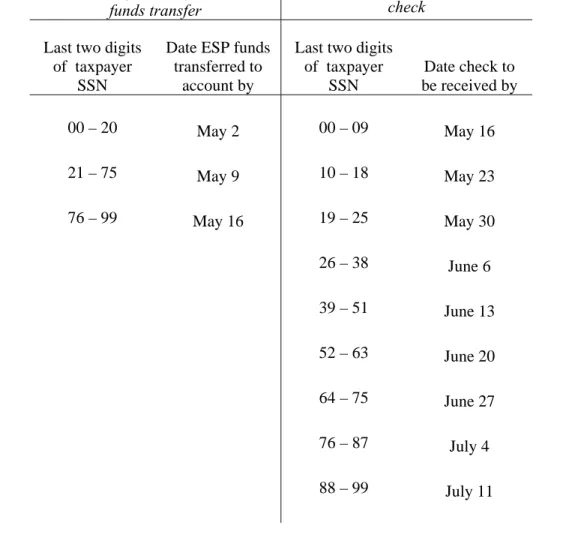
In terms of timing, the disbursement of ESPs over time was effectively randomized conditional on disbursement by paper check or direct deposit. Within each method of delivery, the week that the payment was disbursed was determined by the last two digits of the recipient’s Social Security number, which we treat as random as discussed in the introduction. For recipients that had provided the IRS with their personal bank routing number (i.e., for direct deposit of tax refunds), the stimulus payments were disbursed electronically over a three-week period ranging from the end of April to the middle of May.9 The IRS mailed a statement to each household informing it about the deposit a few business days before the electronic transfer of funds.10 The online supplementary appendix contains an example of this letter. For recipients that did not provide a personal bank routing number, the ESPs were disbursed by paper checks
7
See Auerbach and Gale (2009) for a description of fiscal policy in 2008.
8
All income information was based on tax returns for year 2007. If subsequently a household’s tax year 2008 data implied a larger payment, the household could claim the difference on its 2008 return filed in 2009. However, if the 2008 data implied a smaller payment, the household did not have to return the difference.
9
The ESP was directly deposited only to a personal bank account, a debit card, or a “stored value card” from a personal tax preparer. The payment was mailed for any tax return for which the IRS had the tax preparer’s routing number, as for example would occur as part of taking out a refund anticipation loan or paying a tax preparation fee from a refund. These situations are common, representing about a third of the tax refunds (not rebates) delivered via direct deposit in 2007.
10
Banks also were notified a few days before the date of funds transfer, and some banks showed the amount on the beneficiary's bank account a day or more before the actual credit date. For example, some EFTs deposited on Monday April 28 were known to the banks on Thursday April 24, and some banks seem to have credited accounts on Friday.
7
over a nine-week period ranging from the middle of May to the middle of July.11 The IRS sent a notification letter one week before the check was mailed. Table 1 shows the schedule of ESP disbursement.
According to the Department of the Treasury (2008), $78.8 billion in ESPs were disbursed during the second quarter of 2008, which corresponds to 2.2% of GDP or 3.1% of personal consumption expenditures in that quarter, and $15 billion in ESPs were disbursed during the third quarter, which corresponds to about 0.4% of GDP or 0.6% of personal consumption expenditures.
3. NCP Household-level data on expenditures and ESP receipt
The relation between ESPs and expenditures is measured using information from Nielsen’s Consumer Panel (NCP) for 2008 (formerly Nielsen’s Homescan Consumer Panel), a survey of U.S. households that tracks spending mainly on household goods with Universal Product Codes (UPCs, referred to as “barcodes”). 12 These data have four main advantages for our purposes.
First, the sample of household is much larger than in comparable panel datasets that measure household spending. While there were about 120,000 households in the consumer panel at any point in 2008, only about half of these households meet the static reporting requirement used by Nielsen to define actively participating households for the period January to April 2008. This implies that the regular reporting NCP panel has just under ten times the number of households as the Consumer Expenditure Survey (CEX) for example.
Second, the amount of spending is measured relatively accurately because of a short recall window and the survey technology. Spending data are collected electronically through the use of barcode scanners. Households in the NCP are given barcode scanners and asked to use
11
Taxpayers who filed their tax returns after April 15 received their ESPs either in their allotted time based on their SSN, or as soon as possible after this date (about two weeks after they would receive a refund). Taxpayers filing their return after the extension deadline, October 15, were not eligible for ESPs. Since 92 percent of taxpayers typically file at or before the normal April 15th deadline (Slemrod et al., 1997) and the vast majority of late returns occur close to the extension deadline, there should be very few EPSs that are distributed during the main program that have their distribution date set by the lateness of the return. Finally, due to an error, about 350,000 households (less than 1%) did not receive the child tax credit component of their ESP with their main ESP. The IRS disbursed paper checks for the missing amounts starting in early July. Since we only survey households about the first ESP received, this non-randomized second ESP is not in our data. Some of our households might have been surprised by the small size of their first ESP.
12
The data employed in this study is a combination of data licensed from Nielsen and data available through the Kilts-Nielsen Marketing Data Center at the University of Chicago Booth School of Business. The Kilts-Nieslen data are available at http://research.chicagobooth.edu/nielsen/
8
them after each shopping trip for household items to report the total amount spent and to scan in the barcodes of the purchased items. In exchange for regularly uploading information, participants are entered in prize drawings and receive Nielsen points that can be accumulated and used to purchase prizes from a catalogue. Participants also get newsletters and personalized tips and reminders via email and/or mail. Low performing households are dropped. About 75% of Nielsen households are retained from year to year. Both the compensation for regular reporting and the use of scanners in real time increase the accuracy of reported expenditures.
Third, the timing of spending is also well measured by the NCP. Spending is reported on a daily basis, and is collapsed to weekly to match the frequency of ESP disbursement. Accurate measurement of both Payments and spending at this high frequency increase the statistical power of our analysis.
The final advantage of the NCP is that Nielsen has in place a system to survey the households in the NCP. Nielsen typically uses these supplemental surveys to conduct marketing studies for corporate clients. Our survey, described shortly, uses this technology to collect information about the receipt of the ESPs.
In other ways the NCP data are comparable to those available in other surveys. Toward the end of each calendar year, households are surveyed about a number of characteristics including demographics and income in the previous calendar year. The sample is not representative, but, when recruiting participants, Nielsen seeks to add new households with characteristics that make the panel more representative across cells in nine demographic dimensions – including family structure, four income groups, and three occupation categories – to match the 2000 Census population in each cell.13 Nielsen also produces weights that scale up the observed number of households in each cell to be representative by cell.
The NCP panel has one significant disadvantage for this analysis: the scope of spending that it covers is limited to spending on trips to stores to buy household items. The detailed spending data is limited to goods with barcodes, which are concentrated in grocery, drugstore and mass-merchandise sectors, and so the recorded expenditures primarily cover goods such as food and drug products, small appliances and electronic goods, and mass merchandise products excluding apparel. Our analysis uses information on reported trip totals rather than the large amount of detail available on products (approximately 700,000 different goods are purchased at
13
9
some point by household in the sample), which has the advantage of capturing a larger amount of spending. But to put this issue in perspective, (weighted) spending per capita in the NCP is about $57/week which is about 10 percent of NIPA per capital PCE. At the household level, spending is 35 percent of spending on broad nondurable goods reported in the 2008 CE Survey, or 19 percent of total consumption spending.14 As a result, to measure aggregate responses, dollar spending responses are scaled up to a measure of total spending, as described in Section 6.
Our supplemental survey was fielded in multiple waves, with each wave following the standard procedures that Nielsen uses to survey the consumer panel households. For households with Internet access and who were in communication with Nielsen by email, the survey was administered in three waves in a web-based form; for households without access and in contact with Nielsen by US mail the survey was administered in two waves in a paper/barcode scanner form, since the distribution time was slower and the preparation time greater. Repeated surveying was conditional on earlier responses.
The survey has two parts, each of which was to be answered by “the adult most knowledgeable about your household's income tax returns.” Part I (household characteristics) contains a question asking households about their liquid assets (as well as four other questions about behavior not used in this paper). Households completing Part I of the survey in any wave were not asked Part I again. Part II first describes the ESP program and then asks “Has your household received a tax rebate (stimulus payment) this year?” Households responding “Yes” were then asked about the amount and date of arrival of their ESP, whether it was received by check or direct deposit, when they learned that they were getting the payment, and the amount of spending that receipt caused across categories of goods. Households reporting ESP information were not re-surveyed.15 Households responding “No, and we are definitely not getting one” were not asked further questions and received no further surveys. Households responding “No, but we are expecting to,” or “No, and I am unsure whether we will get any,” or “Not sure/don’t know” were not asked further questions but were re-surveyed with Part II (if not the final wave).
14
The NCP expenditure data cover around 40 percent of all expenditure on goods in the CPI. Note, this is not a statement about the dollar share of these goods relative to the dollar cost of one “basket” of CPI. In contrast, the Consumer Expenditure Survey covers about 85 percent of household expenditures. See Broda and Weinstein (2008).
15
The survey thus only measures the first ESP received by a household, or, if more than one was received prior to answering Part II of the survey, the household was instructed to report the larger. The decision not to allow reporting multiple ESP’s and not to re-survey households that report ESP’s significantly reduced the cost of the survey at the cost of missing only a few ESP’s. In the CEX for example, only about 5% of households and 10% of recipients report receiving multiple ESP’s.
10
In terms of timing, the surveys covered the main period during which ESPs were distributed with random timing.16 The online supplementary appendix gives the time-plan, contact letter and email, mail and on-line surveys, and response rates.
The repeated nature of the survey implies that the recall window for the ESP is relatively short: one month for the email/web survey and just over one and a half months for the mail/scanner survey. The survey was administered to all households meeting a Nielsen static reporting requirement for January through April 2008, which amounted to 46,620 households by email/web and 13,243 by mail/barcode scanner.17 For both types of survey, the response rates were 72% to the first wave, and 80% after all waves, giving 48,409 survey responses (of which some are invalid).
The analysis drops all households that: i) do not report receiving an ESP (roughly 20 percent of the respondents); ii) do not report a date of ESP receipt; iii) report not having received an ESP in one survey and then in a later survey report receiving an ESP prior to their response to the earlier survey; iv) report receiving an ESP after the date they submitted the survey; v) report receiving an ESP by direct deposit (by mail) outside the period of the randomized disbursement by direct deposit (mail), and households not reporting means of receipt and reporting receiving an ESP outside both periods of randomized disbursement. With respect to this last cut, we allow a two day grace period for reporting relative to survey submit dates, and a seven day grace period for misreporting relative to the period of randomization (and do not adjust the reported date of receipt). These cuts reduce the sample to 28,937 households. This selection is not random. But it is (presumably) uncorrelated with the randomization, and so creates no bias for estimation of the average spending effect in the remaining sample. Given heterogeneity in treatment effects however, invalid survey responses may create bias for population inference if there are
16
On May 29, 2008, households that had access to the Internet were sent by email a request to take the survey with a link, the amount of Nielsen points they would earn by participating, and the deadline by which they must respond. Those who had not responded were sent reminder emails with links on May 30, June 5, and June 11 and the survey wave closed on June 16. Those households not responding and those whose responses dictated that they should be re-surveyed with Part II of the survey were re-surveyed in a second wave with an email request on June 26, received up to three reminders, and had the survey close on July 16. A third wave of the on-line survey ran from July 25 to August 18. Households that did not have access to the Internet were first sent surveys by mail on June 18, received up to five reminders by telephone conditional on non-response (roughly every 6 days with the last one on July 17), and the survey closed on July 19. Non-respondents and those whose responses dictate it were re-surveyed in a second wave mailed on July 25, received up to five reminders, and the survey closed on September 9, 2008.
17
Thus we survey 79% by email/web. According to the October 2009 Current Population Survey, 69% of households have computer access at home (U.S. Census Bureau, Population Division, Education & Social Stratification Branch http://www.census.gov/population/www/socdemo/computer/2009.html).
11
differences in treatment effects between these dropped households and those not dropped. The maintained assumption is that this bias is small enough to be neglected.
These responses are merged with the information on total spending on each trip taken by each household during 2008 from the KILTS NCP which includes only households that meet the Nielsen static reporting requirement for all of 2008. These data are made weekly and weeks in which no expenditures are reported are considered to be weeks with zero expenditures.18 All analysis uses the population weights that Nielsen produces for the sample of households that meet the NCP static reporting requirement for expenditures for the year 2008.
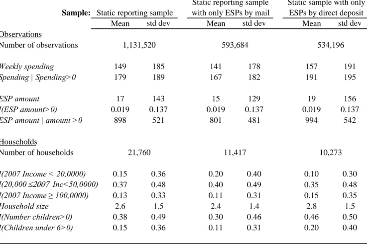
Table 2 shows summary statistics for the data and sample used. Average (weighted) weekly spending in the baseline, static sample is $149. The weekly spending of households receiving ESPs by mail is $16 less than that of households receiving an ESP by direct deposit. The average ESP conditional on receiving one is $898. Households receiving ESP by direct deposit on average have higher ESPs by about $190, consistent with their having on average 0.4 larger households.19
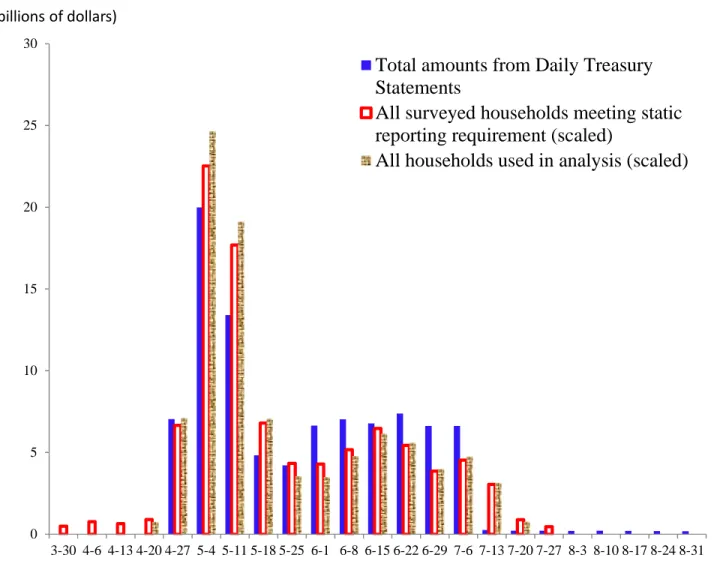
How accurate are these data on ESPs? First, many features of the distribution of the amount and timing of ESPs (documented in Tables A and B in online supplemental appendix) match statistics from similar surveys in the SIPP and the CE. For example, the pattern of Payment amounts cluster at multiple of $300; the average ESP in the CE Survey is $940; and the average ESP received by direct deposit is $180 more than the average received by check.20 Second, one way to judge the representativeness of the sample and how well the survey measures Payments is to compare the weighted, summed survey ESPs to the known aggregate amounts disbursed as reported in the Daily Treasury Statements during the same period. Rescaling household weights to account for missing data, the weighted sample contains 65 billion in reported Payments as compared to the 91 billion that the Treasury reports disbursing over the same period. Finally, to compare timing, Figure 2 plots the weekly distribution over time in Figure 2, where to focus on timing, the NCP weekly amounts are rescaled so that the sum of NCP ESPs matches the sum of DTS EPS’s. The survey of NCP households captures the same
18
With the one exception that if a household stops reporting expenditure during 2008 we consider spending missing rather than zero for the final weeks of the year with zero reported spending. This has almost no effect on the results. The average number of weeks of valid data is 51.7 and the minimum 40.
19
Each additional child eligible for the CTC leads to $300 larger ESP, while most married couples receives $600 more than the equivalent single-headed household.
20
The average household sizes, both among recipients and on-time recipients, are very similar to those in the CEX Survey. These distributions for the CE are reported in Parker, Souleles, Johnson, and McCelland (2011).
12
temporal pattern of disbursement as the Treasury reports. The NCP survey displays a slightly higher share of Payments disbursed by electronic deposit and a slightly lower share later disbursed by mail than the Treasury data.
4. Estimation methodology
Our analysis uses the following regression equation to estimate the average impact of the receipt of an ESP on spending for household i in week t receiving a payment by method m:
Ci,t = µi + (L) ESPi,t + m,t + i,t (1)
where Ci,t is either the dollar amount of spending in week t for household i or the ratio of that
level of spending to the average weekly spending of that household during 2008 prior to the ESP disbursements (the first twelve weeks of the year). µi is a household-specific intercept that
captures differences in spending across households. ESPi,t, the key stimulus payment variable, is
either a dummy variable indicating whether any payment was received by household i in week t or that dummy variable times the average amount of the ESP received, where the average is different by method of receipt m. (.) is a lead and lag polynomial (L is the lag operator), so that (L) ESPi,t represents the sum of a coefficient times the contemporaneous ESPi,t and a series of
coefficients times lags and potentially leads of ESPi,t . To ensure consistency, the (L) cover all
possible lags in the sample. The (L) are the key parameters of interest and measure the spending effects of the ESP prior to its arrival, upon its arrival, and following its arrival. The variable m,t is an indicator variable for the method of disbursement (whether the household reported an ESP delivered by mail or by direct deposit) interacted with an indicator variable for each week. Thus,
m,t is an effect which absorbs any seasonal or average changes in spending for each group of recipients separately in each week. Finally, i,t captures all expenditures unexplained by the
previous factors. Standard errors are adjusted to allow for arbitrary heteroskedasticity and within-household serial correlation.
Consistent estimation of the causal impact of receipt on spending requires that the variation in ESPi,t be uncorrelated with all other factors that might influence household
expenditure besides the receipt-driven variation of interest. Since the timing of the ESP mailing is effectively random, our results exploit only variation in timing of ESP receipt (not amount) among recipients in each method of disbursement. Equation (1) does this by i) using only timing variation in ESP within each means of receipt, ii) removing individual effects to remove
13
differences in the average level of spending, and iii) controlling for the average spending of recipients by mail and recipients by direct deposit separately in each period. Selection into method of disbursement raises the possibility of correlation between type and average treatment effect. With this specification, such a correlation would not bias estimates of average effects within type, nor of the average effect across the two groups.
To interpret the product of the amount disbursed and (L) as the causal increase in aggregate consumption demand further requires that the time effects, m,t are not lowered during the period of disbursement by the (partial-equilibrium) receipt of the Payments.21 While the increase in spending caused by the receipt of an ESP must be offset by lower spending at some point for each household, the maintained assumption is that this lower spending is tied to the timing of the disbursement and so measured in (L) or occurs after our period of estimation. To elucidate this assumption, consider the following counterexample. Suppose that households all changed the timing of their consumption to match the arrival of their EPS’s, but from within the common period of disbursement, so that households that receive their ESPs early in the program on average accelerate spending while households that receive their ESPs late in the program on average delay it. In this case, (L) estimates the causal effect of a Payment on an individual household’s spending but aggregate spending during the period of disbursement is unchanged (because everyone just moves their spending around within a brief, common interval of calendar time). While such heterogeneity in treatment effect (dynamically correlated with the random treatment) is possible, we know of no existing model of consumer behavior that would generate this behavior.
In addition to studying the average treatment effect, equation (1) is also estimated separately for different households by characteristics like asset levels or income levels. The main question of interest for future modelling of household behavior is whether there are differences in average treatment effect across households with different characteristics.
Selection into the NCP and/or nonrandom missing data would bias population inference of average treatment effects if it were correlated with treatment effect. While the experiment provides randomization that aids identification, our analysis can only estimate the causal effect of ESP receipt for the population of households represented by those in the NCP that respond to
21 There may be a drop in this time effect (m,t) due to general equilibrium effects of course, but that does not change
14
our survey with valid responses. Use of the NCP weights ensures that the sample is representative along several observable measures, but the potential for bias remains. 22
While finding a significant effect of ESP receipt on spending represents a rejection of the canonical consumption smoothing condition of the frictionless, textbook lifecycle/permanent income hypothesis (LCPIH), this experimental methodology is distinct from tests of the LCPIH based on the Euler equation. Euler equation estimation uses time-series moments derived from first-order conditions to test the null hypothesis/moment restriction that the effect of an anticipated income change on spending is zero. Instead, this paper uses the randomized timing of ESP receipt to provide orthogonality between the residual and the timing of ESP receipt. This alternative approach allows estimation of the causal effect of the receipt of a pre-announced income change on spending independent of the theory being tested. Our approach does still provide a direct test of the rational expectations LCPIH without constraints since the passage of ESA 2008 predates the experiment.
5. The average response of spending to the receipt of an ESP
This section begins by identifying the average effect of the receipt of an ESP on weekly spending in the sample of all households from all available variation in timing, including that due to different method of disbursement, so m,t =t in equation (1). The first three columns of Table
3 display estimates of (.) – the coefficient on the one included lead, the contemporaneous ESP variable, and the first three lags (of the complete set of included lags).
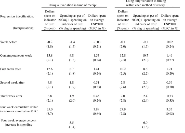
First, on average, there is a highly statistically significant increase in spending on NCP household goods upon arrival of an ESP. For example, the first column reports coefficients from a regression of total spending (in dollars per week) on the lead and lag polynomial of an indicator variable for week of ESP receipt so that the reported coefficients are interpreted as the dollar spending caused by the receipt of an ESP in that week. Households on average increase their spending by a reasonably precisely estimated 13.8 dollars in the week that the ESP arrives. The second column show the results of switching the dependent variable to dollars spent as a percent of average weekly spending in the first 12 weeks of the year, which gives a spending effect in the week of arrival of 9.8 percent of average weekly spending. These estimates are
22 Another assumption, implicit in (L) not varying with t, is that any time-variation in the treatment effect is not
15
consistent with each other in the sense that a 9.8 percent response at the average weekly spending level of $149 implies a spending response of $14.60.
The third column reports the most important specification for later analysis. Dollar spending is regressed on the lead/lag polynomial of the indicator variable for receipt times the average amount of ESP for all households, which gives β(L) the interpretation of a marginal propensity to consume out the rebate (MPC). Thus, these coefficients measure the average propensity to spend out of the ESP. In the week that the ESP arrives, its arrival causes a highly significant increase in spending of 1.53 percent of the ESP. At the average ESP amount of $898, this would be a response of $13.74.
There is no evidence of any greater spending in the week before the arrival of the ESP in any specification. This lack of pre-treatment effects also suggests that there is very little reporting error in date of receipt, as for example due to recall error, at least after dropping the clearly erroneous reports.
While there is no spending effect of receipt immediately before receipt, there is a continued spending effect for weeks after receipt. This spending effect declines slightly the week after arrival and continues declining reasonably smoothly so that the coefficients on weekly spending in all specifications are no longer individually statistically significant by the third week. The last row of the table reports the spending effects over the four weeks starting the week of receipt: the cumulative dollar spending is $35, the percent increase in spending over the period is 5.5 percent of spending, and the total share of the ESP spent is 3.9 percent.
The second triplet of columns in Table 3 show the results of estimating the same three specifications but now treating the two different methods of disbursement as two separate experiments, as in equation (1). The results in the second three columns are very similar to those in the first three columns. Using only experimental variation in timing, the point estimates of the contemporaneous spending effect of receipt are slightly lower but still highly significant: 13 dollars, 11 percent of spending, and 1.5 percent of the ESP on average. There are no significant spending effects prior to receipt. And over four weeks, the cumulative spending effects are highly statistically significant 28 dollars, 6.0 percent of spending, and 3.4 percent of the ESP on average.
These results are reasonably robust. Similar patterns emerge (adjusting for differences in average spending) when restricting to households reporting spending in at least half the weeks or in every week, and when trimming the top and bottom 1% of spending. Similar percentage
16
changes and spending effects relative to average dollar spending are found measuring spending as the (smaller) sum of all individual barcode items reported instead of the (larger) sum of all total trip spending. With this dependent variable, we are also able to use a larger sample of households that includes those that do not meet the Nielsen static reporting requirement for the year, and a weight specially constructed for us by Nielsen for this larger sample. While statistical precision is slightly lower and dollar spending is lower, the pattern of coefficients remains similar as a share of average spending to those reported.
Are there further small but measurable spending effects of receipt of an ESP beyond the first month? To investigate this question, the impulse response to the receipt of an ESP is smoothed by making β(L) constant across four-week periods, starting with the week of receipt. By estimating fewer parameters, longer-term spending effects of the receipt of an ESP may be estimated more precisely.
Table 4 shows the monthly impulse responses of spending to the receipt of an ESP. The increase in spending caused by the receipt of an ESP is estimated to be $42.6 (column 1) or $47.6 (column 4) in the month following receipt, both slightly larger than found in Table 3 (four week increase). After the initial month, spending is estimated to be increased by $9.3 or $26.3 in the first following month, and by $8.6 or $20.5 in the month after that, although only the larger (column 4) estimate in the first month is statistically significant. Measured as percent changes in spending, spending rises by between 5.25 and 6.89 percent the month of arrival, but the lagged effects over the next two months are estimated to be negative in column 2 and economically significant and decaying in column 5. Finally, the third column and the last column of Table 4 show that households spent about five percent of their ESPs the month they arrived and a continued one to three percent over the following two months. Unlike in the analysis at the weekly frequency, there are some economically significant (although not statistically significant) spending effects the month prior to the receipt of an ESP, particularly for the analysis that treats each method of disbursement as a separate experiment (column 4 in particular). This fact combined with the fact that there are no pre-treatment effects in the weekly analysis (and in similar weekly analysis with more leads) suggest that the spending effects in columns 1 and 3 are probably more reliable estimates of the longer term effects than the larger spending effects shown in columns 4 and 6. The estimates of cumulative spending over four weeks reported in Table 3 also support the analysis of columns 1 and 3 over 4 and 6 in Table 4.
17
In sum, our preferred estimates imply that cumulative spending totals over the three months following receipt are 61 dollars, 1.6 or 3.8 percent of average spending, and 7 percent of the ESP amount on average. We now use the results from column 3 of Table 4 to calculate the implications of this ESP program for aggregate demand both in economic models and in reality.
6. The partial-equilibrium, aggregate effect of the stimulus payments
What do these household-level estimates imply for macroeconomic models of fiscal policy and for the efficacy of the actual policy in 2008? This section presents calculations of the change in aggregate consumption demand associated with a given disbursement of stimulus payments. This calculation involves two steps: first scaling the increase in demand for NCP goods to a broad measure of spending on goods and services, and then second aggregating these responses to moments useful for matching by DSGE models or for matching aggregate spending in the spring and summer of 2008.23 As discussed in the introduction, this calculation omits any effects that are not correlated with timing of receipt, and excludes all multiplier effects. This section measures only the effect of receipt on demand.
Scaling spending from just NCP items to spending on more complete measures of consumption expenditures is done in three different ways.
The first method simply multiplies the estimated MPC’s by the ratio of National Income and Product Account (NIPA) quarterly personal consumption spending per capita to NCP quarterly spending per capita. This method has two weaknesses. This method ignores that some aggregate consumption is not discretionary, out-of-pocket spending by households (e.g. consumption of health goods and services) which biasing our estimate of total spending upward. On the other hand, this method ignores that the propensity to spend on NCP goods is likely lower than that on all goods and services, which biases our estimate of total spending downward. NCP purchases that can be categorized (the subset that have barcodes and are scanned in) disproportionately comprise spending on necessities and goods that Johnson, Parker, and Souleles (2006) found to have low MPC’s in response to the 2001 tax rebate (e.g. food at home).
Second, the supplemental ESP survey ended with questions asking each household how they spent their ESP (the survey is in the online supplementary appendix). First, the household was asked the question pioneered by Shapiro and Slemrod (1995), “Thinking about your
23
The existing household-level estimates have already been used by a number of partial-equilibrium models, such as Reis (2006), Huntley and Michelangeli (2014), and Kaplan and Violante (forthcoming).
18
household’s financial situation this year, is the tax rebate leading you mostly to increase spending, mostly to increase savings, or mostly to pay off debt?” The household was then asked five more questions: “For questions #6 through #10, please think about the extra amount you are spending because of this rebate on each type of purchase outlined below . . . How much (in dollars rounded to the nearest dollar) are you spending on each of the following?” The second method scales the estimated MPC’s by the ratio of average reported ESP spending on all goods (sum of questions 6 to 10) to average reported ESP spending on NCP goods alone (question 6).24
The third method is to scale our spending estimates up based on the distribution of spending in the NCP and the total MPC that is due to each category of spending as estimated in the CE data by PSJM. Specifically, Table 6 in PSJM reports the share of total MPC in each category of spending. For each category, this share is multiplied by the ratio of NCP spending to CE spending and summed to provide an estimate of the share of total MPC captured by NCP spending. To calculate NCP spending by category, all purchases that have a comparable CE category are allocated to spending on that category and the remainder of NCP spending is divided evenly among all CE categories except purchases of vehicles (because such purchases would not be reported in the NCP) and food at home, alcoholic beverages, and tobacco products (because such purchases are mostly scanned in and reported in these categories).
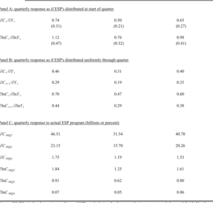
Table 5 reports the results of three calculations for each of these three methods of aggregation. The first two calculations provide statistics useful for disciplining models of consumer behavior embedded in a DSGE model. Panel A assumes that a stimulus program is implemented that distributes stimulus payments in the first week of the quarter, so that all spending effects measured in Table 4 occur within the quarter. The total increase in aggregate demand for consumption is between 50 and 74 percent of the distributed payments. Panel B assumes instead that the payments are distributed evenly across the weeks of a single quarter so that the spending effects of Table 4 are distributed across the current and subsequent quarter. The aggregate response of demand is 31 to 46 percent of the rebate amount during the quarter of disbursement and 19 to 29 percent during the following quarter.
Given heterogeneity in spending response to receipt across households, how should the distribution of Payments across households in a model of spending responses be structured to
24
More complex procedures were tried with essentially the same results. For example, the numbers are almost unchanged if the reported spending amounts are predicted from a regression on household characteristics and then spending is scaled up at the household level.
19
match what actually occurred in this experiment? In 2008, the ESPs were not sent to households with very low or very high incomes in 2007. According to the law, ESPs were not disbursed to household with less than $3,000 of qualifying income in 2007 or who did not file a tax return. And a married couple filing jointly without children would receive no ESP if their AGI exceeded roughly $150,000, which covers the top 14% of families (or 9% of households) by income (according to the ACS). BLS (2009) provides further statistics on the distribution. Relative to a mean household income of $63,200 BLS (2009) reports that 21% of households with income below $10,000 received an ESP and that these ESPs averaged $599. Similarly, 43% of households with incomes over $70,000 (with average income of $130,200) received a Payment and these ESPs averaged $1,227.
Turning to the real world aggregate effects, the estimated increase in demand for goods during and shortly after the program caused by the receipt of the Payments in 2008 is the household-level impulse responses applied to the observed aggregate disbursements of the Payments over time as reported by the Daily Treasury Statements (2008). These calculations imply significant aggregate spending effects. Panel C of Table 5 shows that the disbursement of the ESPs directly raised the demand for consumption by between 1.3 and 1.8 percent in the second quarter of 2008 and by 0.6 to 0.9 percent in the third quarter. These estimates relative to the time series of aggregate consumption spending were presented in Figure 1 in the Introduction. The estimates suggest that consumption spending was maintained during the first 9 months of the recession by the ESP program. Of course whether the ESP program’s effect was larger or smaller than that given by these accounting calculations depends on the extent of the multiplier or crowding out not included in these calculations, and on any other effects of the ESP program on aggregate demand not correlated with the timing of receipt.
The next section considers whether there was any noticeable additional increase in spending when households first learned about their ESPs, while the following section analyzes heterogeneity in spending response by income and liquid wealth.
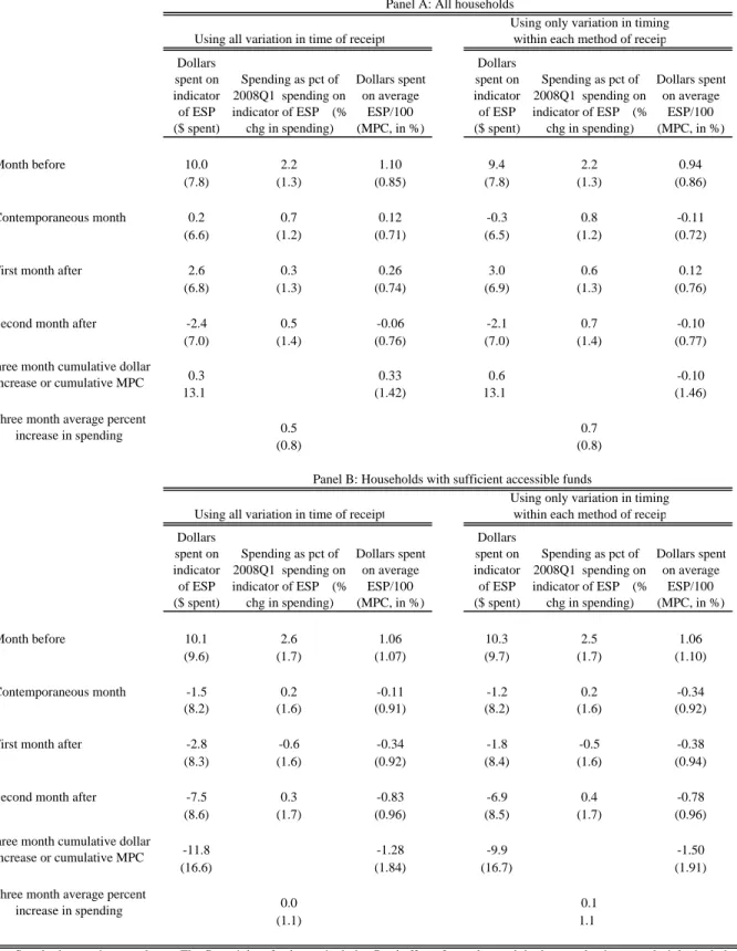
7. The average response of spending to learning about an ESP
This section investigates whether households increased their spending on NCP-measured goods at the different times at which they learned about their ESPs. After households reported receiving an ESP, the ESP survey asked “Was this about the amount your household was expecting?” Households could respond, “no and we were surprised to get any rebate at all,” “no
20
and it was less than we were expecting,” or “no and it was more than we were expecting.” They could also respond “yes, and we’ve known the approximate amount since February,” and the same with “since March,” “since April,” and “yes, but we only learned about it recently.” Finally a household could respond “not sure/don’t know.”
To measure the spending effect of learning about a Payment, equation (1) is estimated but with an indicator variable for the month in which the household learned about their ESP (denoted
LESP) instead of an indicator variable for receipt.25
Households who report ‘don’t know’ or that they were negatively surprised are dropped. This method thus compares the spending of households that learned about the ESPs in different months prior to arrival. Since the variation is monthly, β(L) is set to monthly. While this analysis exploits variation in timing to measure a spending effect, unlike in the previous section, this variation in timing is not random and so is possibly correlated with other reasons for temporal changes in spending.
Panel A of Table 6 shows that there is very little evidence of any spending response. Analogous to previous tables, the regressions reported in columns 1, 2, 4 and 5 include distributed lags of the indicator for the month in which the household learns about the ESP, while columns 3 and 6 include distributed lags of the average ESP amount times this variable. All estimated effects are economically small and statistically insignificant.
Why are there no measureable responses? First, it is always possible that the self-reported recall about learning is poor. Second, and perhaps more important, the LCPIH predicts only a small increase in lifetime resources associated with the ESP and so only an economically small spending response.
Third, some household might not respond to news about future income due to liquidity constraints or high costs of borrowing so that in the population of constrained and unconstrained households there is no noticeable response. If so, the spending response may be larger in a sample restricted to households who have access to liquidity. Part I of the supplemental survey asked households “In case of an unexpected decline in income or increase in expenses, do you have at least two months of income available in cash, bank accounts, or easily accessible funds?” Note that this question is asked of households when they are first surveyed, potentially before they report receiving an ESP in a later survey, but after the period in which most variation in learning about ESPs occurs. Panel B of Table 6 repeats the analysis of Panel A but only for
25
The sample is restricted to data before the first full week of July. The results are very similar if the sample in instead restricted to the first 18 weeks of the year to avoid the period of the main experiment entirely.
21
households who answer that they have sufficient funds. Even for households with adequate liquid wealth, there is no evidence of any spending response upon learning about the ESP, although as noted, the variation is not exogenous and the LCPIH would predict little spending response.
In sum, there is no evidence of a quantitatively important increase or decrease in spending by households when they learn about their ESPs.
8. Heterogeneity in the response of spending across households
This section investigates the differential spending response of households across 2007 income levels and across different levels of liquid wealth. Temporarily low income may indicate low liquidity and a high propensity to consume. Alternatively, low income may indicate greater impatience or other characteristics of people who are more (or less) likely to spend income when it arrives. Similarly, low liquidity when combined with sufficiently high impatience or expected increases in income may indicate that a household is liquidity constrained and has a high propensity to consume from expected income increases.
To investigate the role of liquid wealth and income, equation (1) is estimated separately on subsets of households grouped by income and liquidity. Because there are differences in the average ESP and average spending level across groups of households with different levels of income and liquidity, the specifications that use only indicators of receipt may estimate different amounts of spending because average spending differs across groups or because the average dollar amount of the ESPs differ across group, rather than because behavior differs by group. As a result, this section focuses on the specification that regresses dollars spent on the average amount of the ESP by group, which is the specification estimating the propensity to spend in each group.
In the NCP, income is measured in ranges and 2007 annual income is reported at the beginning of 2009. For our analysis, households are divided into three groups that represent, in the weighted data, the bottom 35% of households, the middle 34%, and the top 30%. Table 7 show that the bottom third of households by income – those with annual labor incomes of less than $35,000 – consume at greater rates than the other groups. Focusing on the second triplet of columns in both Panel A and Panel B, in the month of arrival, the propensity to consume of the bottom income group is roughly double that of the middle and top income groups. But these differences narrow over time. By three months after receipt, households in the bottom third of
22
the distribution of 2007 income have consumed a similar share of their ESP as those in the top third, a both economically and statistically significant 13 – 15 percent of their ESPs on NCP goods. This is in contrast to households in the middle of the income distribution whose MPC is significantly lower. That is, as found in Parker (1999) there is weak evidence that high-income households smooth consumption as poorly as low income households over predictable income changes of this size. Finally, because the amount of the ESP increases with income, the total dollar spending across households is not as different across income groups (first three columns of both Panel A and Panel B of Table 7).
Turning to liquidity, Part I of the survey contains the question “In case of an unexpected decline in income or increase in expenses, do you have at least two months of income available in cash, bank accounts, or easily accessible funds?” and the respondent can answer yes or no. In the weighted sample, 41 percent of households answers that they do not have this much liquidity.
Table 8 shows that spending responses are concentrated among those households without sufficient liquidity. In the first month, the receipt of an ESP causes households without access to sufficient funds to spend roughly 9 percent of their ESPs on NCP goods, which is three to four times the amount spent by households out sufficient funds. In the months following, these differences narrow only slightly, so that in both Panels A and B, illiquid households spend more than twice as much of their ESPs over three months following receipt as households reporting sufficient liquidity. This conclusion is also visible in the dollar spending caused by the arrival of an ESP, displayed in the first two columns in each Panel, with illiquid households spending triple the dollar amount on arrival of illiquid households and more than double the amount over a three month period.
9. Conclusion
In normal times, monetary policy is the main instrument of stabilization policy arguably because the effects of monetary policy are reasonably well understood and because central banks can react rapidly to the possibility of a recession. But monetary policy has limitations – lags in its effect, increases in inflation, and reduced efficacy when financial institutions are capital-poor or when the zero lower bound on nominal interest rates binds. At such times, fiscal policy in the form of tax rebate programs have been able to respond quickly and temporarily to economic slowdowns. But the increased use of tax rebate programs raises two central questions. First, do
23
these programs generate more spending? And second, does this spending have social benefits that exceed the future costs of the program?
This paper uses novel data to speak directly to the first question. At the household level, spending on NCP goods spikes up by ten percent the week in which an ESP arrives. Continued spending implies that spending is roughly 6 percent higher over the month starting with arrival and 3 to 5 percent higher the three-month period starting with arrival. To move to aggregate effects, these results are aggregated across households and extrapolated to include spending on unobserved goods and services.
In terms of macroeconomics models, these calculations imply that in a quarterly model, the propensity to consume at the individual level from an equivalent tax rebate in a quarter is between 50 and 75 percent. In a more realistic continuous-time or higher-frequency model, if tax rebates were uniformly distributed during a quarter, the average partial-equilibrium spending response would be 30 to 45 percent of the rebate amount during the quarter of disbursement and 20 to 30 percent during the following quarter. In terms of the real world, the disbursement of the ESPs directly raised the demand for consumption by between 1.3 to 1.8 percent in the second quarter of 2008 and by 0.6 to 0.9 percent in the third quarter of 2008, with ranges reflecting differences across scaling factors.
This paper speaks only indirectly to the second question. Our results imply that DSGE-based calculations of the efficacy of fiscal policy should incorporate a share of households that spend significant amounts of transfers when they arrive, a modeling assumption that would imply behavior substantially different than the Ricardian assumptions typically embodied in DSGE models used to evaluate fiscal policies.
24
References
Agarwal, S., Liu, C., Souleles, N.S., 2007. The Response of Consumer Spending and Debt to Tax Rebates – Evidence from Consumer Credit Data. Journal of Political Economy 115, 986-1019.
Auerbach, A.J., Gale, W.G., 2010. Activist Fiscal Policy to Stabilize Economic Activity. In: Federal Reserve Bank of Kansas City, Financial Stability and Macroeconomic Policy: A Symposium. Federal Reserve Bank of Kansas City, pp. 327- 374.
Bertrand, M., Morse, A., 2009. What do High-Interest Borrowers Do with their Tax Rebate?” American Economic Review 99, 418-423.
Blinder, A.S., 1981. Temporary Income Taxes and Consumer Spending, Journal of Political Economy 89, 26-53.
Broda, C., Parker, J.A., 2008. The Impact of the 2008 Tax Rebates on Consumer Spending: Preliminary Evidence. Kellogg School of Management working paper, July.
Broda, C., Weinstein, D., 2008. Product Creation and Destruction: Evidence and Price Implications. American Economic Review 100, 691-723.
Browning, M., Lusardi, A., 1996. Household Saving: Micro Theories and Macro Facts. Journal of Economic Literature 34, 1797-1855.
Bureau of Labor Statistics, U.S. Department of Labor, 2009. Consumer Expenditure Survey Results on the 2008 Economic Stimulus Payments (Tax Rebates), October (http://www.bls.gov/cex/taxrebate.htm).
CCH, 2008. CCH Tax Briefing: Economic Stimulus Package. February 13.
Coronado, J.L., Lupton, J.P., Sheiner, L.M., 2005. The Household Spending Response to the 2003 Tax Cut: Evidence from Survey Data. Finance and Economics Discussion Series 2005-32. Board of Governors of the Federal Reserve System (U.S.).
Deaton, A., 1992. Understanding Consumption. Oxford: Clarendon Press.
Evans, W.N., Moore, T.J., 2011. The Short-Term Mortality Consequences of Income Receipt. Journal of Public Economics 95, 1410-1424.
Feldstein, M., 2008. The Tax Rebate Was a Flop. Obama's Stimulus Plan Won't Work Either” The Wall Street Journal, August 6.
Flavin, M., 1981. The Adjustment of Consumption to Changing Expectations about Future Income. Journal of Political Economy 89, 974-1009.
25
Evidence from Tax Rebates. Review of Economics and Statistics 96, 431-443.
Hsieh, C., 2003. Do Consumers React to Anticipated Income Changes? Evidence from the Alaska Permanent Fund. American Economic Review 99, 397-405.
Huntley, J., Michelangeli, V., 2014. Can Tax Rebates Stimulate Consumption Spending in a Life-Cycle Model? American Economic Journal: Macroeconomics 6, 162-89.
Jappelli, T., Pistaferri, L., 2010. The Consumption Response to Income Changes. Annual Review of Economics 2, 479-506.
Johnson, D.S., Parker, J.A., Souleles, N.S., 2006. Household Expenditure and the Income Tax Rebates of 2001. American Economic Review 96, 1589-1610.
Johnson, D.S., Parker, J.A., Souleles, N.S., 2009.The Response of Consumer Spending to Rebates During an Expansion: Evidence from the 2003 Child Tax Credit. working paper, April.
Kaplan, G., Violante, G., 2011. A Model of the Consumption Response to Fiscal Stimulus Payments. Econometrica 82, 1199-1239.
Parker, J.A., 1999. The Reaction of Household Consumption to Predictable Changes in Social Security Taxes. American Economic Review 89, 959-973.
Parker, J.A., Souleles, N.S., Johnson, D.S., McClelland, R., 2011.Consumer Spending and the Economic Stimulus Payments of 2008. NBER working paper 16684, Cambridge, MA. Parker, J.A., Souleles, N.S., Johnson, D.S., McClelland, R., 2013. Consumer Spending and the
Economic Stimulus Payments of 2008. American Economic Review 103, 2530-53.
Poterba, J.M., 1988. Are Consumers Forward Looking? Evidence from Fiscal Experiments. American Economic Review 78, 413-418.
Reis, R., 2006. Inattentive Consumers. Journal of Monetary Economics 53, 1761-1800.
Sahm, C.R., Shapiro, M.D., Slemrod, J.B., 2010. Household Response to the 2008 Tax Rebates: Survey Evidence and Aggregate Implications. In: ed. Brown, J.R. (Ed.), Tax Policy and The Economy, 24. MIT Press, Cambridge MA, 69-110.
Shapiro, M.D., Slemrod, J.B., 1995. Consumer Response to the Timing of Income: Evidence from a Change in Tax Withholding. American Economic Review 85, 274‐283.
Shapiro, M.D., Slemrod, J.B., 2003. Consumer Response to Tax Rebates. American Economic Review 85, 274-283.
Shapiro, M.W., Slemrod, J.B., 2009. Did the 2008 Tax Rebates Stimulate Spending?” American Economic Review 99, 374-79.
26
Slemrod, J.B., Christian, C., London, R., Parker, J.A., 1997. April 15 Syndrome. Economic Inquiry 35, 695-709.
Souleles, N.S., 1999. The Response of Household Consumption to Income Tax Refunds. American Economic Review 89, 947-958.
Souleles, N.S., 2002. Consumer Response to the Reagan Tax Cuts. Journal of Public Economics 85, 99-120.
Stephens, M. Jr., 2003. 3rd of tha Month: Do Social Security Recipients Smooth Consumption Between Checks? American Economic Review 93, 406-422.
Stephens, M. Jr., 2006. Paycheck Receipt and the Timing of Consumption. The Economic Journal 116, 680-701.
Taylor, J.B., 2010. Getting Back on Track: Macroeconomic Policy Lessons from the Financial Crisis. Federal Reserve Bank of St. Louis Review 92, 165-176.
Department of the Treasury, 2008. Daily Treasury Statement. Washington: GPO, various issues. Wilcox, D.W., 1990. Income Tax Refunds and the Timing of Consumption Expenditure.
working paper, Federal Reserve Board of Governors.
Zeldes, S.P., 1989a. Consumption and Liquidity Constraints: An Empirical Investigation. Journal of Political Economy 97, 305-346.
Zeldes, S.P., 1989b. Optimal Consumption with Stochastic Income: Deviations from Certainty Equivalence. Quarterly Journal of Economic 104, 275-298.