Calculation of Radiation from a Helically Cut Waveguide for a Gyrotron Mode Converter in the Quasi-Optical Approximation

(1)

Plasma Science and Fusion Center Massachusetts Institute of Technology

Cambridge MA 02139 USA

(submitted to IEEE Trans. Plasma Science, September, 2007)

This work was supported by the U.S. Department of Energy, Grant No.

DE-FC02-93ER54186. Reproduction, translation, publication, use and disposal, in whole or in part,

PSFC/JA-07-17

Calculation of Radiation from a Helically Cut

Waveguide for a Gyrotron Mode Converter in the

Quasi-Optical Approximation

(2)

APS/123-QED

Calculation of Radiation from a Helically Cut Waveguide for a

Gyrotron Mode Converter in the Quasi-Optical Approximation

E. M. Choi*, M. A. Shapiro, J. R. Sirigiri, and R. J. Temkin

(Dated: August 21, 2007)

Abstract

A gyrotron internal mode converter consists of a launcher that radiates the waveguide mode as a nearly Gaussian beam in free space, followed by a set of mirrors to focus and direct the radiation. We present a calculation of the radiation from the launcher based on a quasi-optical approach that includes diffraction. The results are in good agreement with a calculation using a numerical code based on the electric field integral equation approach. The results should be useful for designing so-called Vlasov internal mode converters and for understanding the role of diffraction in the design of internal mode converters for gyrotrons.

(3)

I. INTRODUCTION

High power gyrotron cavities operate in high order transverse electric (TE) modes of a waveguide with an axial wavenumber close to cutoff ([1], [2]). It is important to convert these high order TE modes into a low order waveguide mode or a Gaussian-like beam in free space in order to reduce losses in the transmission of the gyrotron output power. Present day gyrotrons operating at very high power levels, hundreds of kilowatts to above one magawatt, use a mode converter located inside the gyrotron, a so-called internal mode converter (IMC).

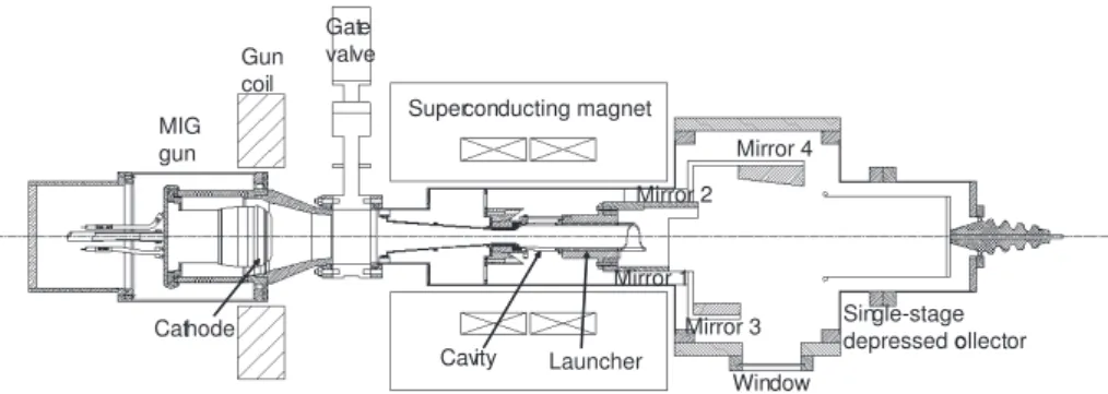
Superconducting magnet Gate valve Gun coil MIG gun Cathode Cavity Launcher Single-stage depressed collector Mirror 4 Mirror 3 Mirror 2 Mirror 1 Window

FIG. 1: A schematic of the 1.5 MW, 110 GHz gyrotron with the internal mode converter.

Fig. 1 shows the schematic of 1.5 MW, 110 GHz gyrotron at MIT. The gyrotron is installed in a superconducting magnet. The electron beam is generated by a magnetron injection gun (MIG) and deposited on to a single-stage depressed collector. The IMC is located after the cavity and operates in a waveguide just above cutoff, thus reducing the size and increasing the efficiency of the converter. The converter is constructed of a launcher, which radiates the power from the waveguide TE mode into a Gaussian-like beam, followed by a series of mirrors that can correct the phase errors of the launched beam. The final microwave beam, which is Gaussian-like, exits the gyrotron through a window.

An internal mode converter consisting of a helically cut waveguide, called a launcher, followed by a set of smooth focusing mirrors was first proposed and demonstrated by Vlasov et al. [3]. The launcher is simple helically cut section of waveguide. The power radiated from the launcher is captured by one or two cylindrical mirrors and converted to a Gaussian beam of good quality. The advantage of this version of the IMC is that it is relatively simple and is very compact. The disadvantage is that the power radiated from the launcher

(4)

contains sidelobes, which limit the IMC efficiency to about 80 %. This low efficiency is unacceptable for megawatt power level gyrotrons. However, the Vlasov IMC is used in low power gyrotrons because it is very compact and easy to fabricate [4]. It is also used external to the gyrotron [5].

Several optimized modifications of the Vlasov antenna have been reported in the literature ([6], [7], [8], [9], [10], [11]). These modifications allow one to improve the efficiency of conversion of a rotating circular waveguide mode into a Gaussian beam. In one of the most successful of these designs, a mixture of modes is generated by a rippled wall prior to the launcher so as to form a Gaussian-like beam with little or no sidelobes, thus allowing very high efficiency in the IMC [9]. In a recent paper, the launcher has been optimized numerically using the surface current integral equation method, leading to close to 100 % theoretical efficiency for the IMC [12].

In this paper, we use the quasi-optical theory of diffraction to calculate the radiation from a helical cut of a waveguide. The case considered applies to the Vlasov launcher and the Vlasov IMC. Analytic results are compared to numerical results obtained from the electric field integral equation method. Since the Vlasov IMC is still in use, the present results should be helpful in designing such converters. The present results will also be useful for understanding the general role of edge diffraction in the gyrotron IMC design ([13], [14]). The quasi-optical approach used in this paper was previously applied to radiowave propagation in the atmosphere and later was extended to laser applications([15], [16], [17], [18]).

II. GEOMETRICAL OPTICS REPRESENTATION FOR A WAVEGUIDE MODE

For a TE waveguide mode, the Helmholtz equation for the axial magnetic field u = Hz is written in cylindrical coordinates (r, φ) as

∂2_u ∂r2 + 1 r ∂u ∂r + 1 r2 ∂2_u ∂ϕ2 + k 2 ⊥u = 0 (1) k⊥ = p k2_{− k}2

z is the transverse wave number. The solution for TEmn modes is

u = Jm(k⊥r)e−imϕ (2)

where m is the azimuthal index.

The geometrical optics solution can be derived within the approximation k⊥rÀ1, mÀ1. We represent the solution of Eq. 1 as u = A(r)e−ik⊥s(r,ϕ), where k

(5)

The second order terms of k⊥ give an eikonal equation, µ ∂s ∂r ¶₂ + 1 r2 µ ∂s ∂ϕ ¶₂ = 1 (3)

and the function s(r, ϕ) is an eikonal. The first order term of k⊥ gives the transfer equation as shown below. 2∂A ∂r ∂s ∂r + µ ∂2_s ∂r2 + 1 r ∂s ∂r + 1 r2 ∂2_s ∂ϕ2 ¶ A = 0 (4) Assuming s(r, ϕ) = f (r) + mϕ_k

⊥, we obtain from Eq. 3

f (r) = Z s 1 − m2 k2 ⊥r2 dr = s r2₋ m2 k2 ⊥ − m k⊥ arccos( m k⊥r ) Therefore, the eikonal is

s(r, ϕ) = s r2 ₋m2 k2 ⊥ + m k⊥ µ ϕ − arccos( m k⊥r ) ¶ (5) From Eq. 4 we obtain the amplitude

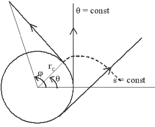
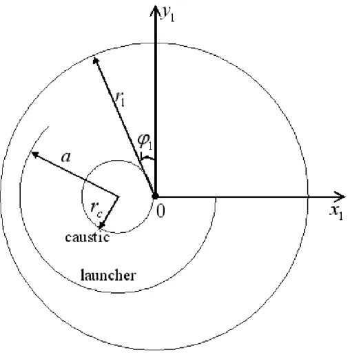
A(r) = µ r2− m 2 k2 ⊥ ¶_−1/4 (6) The geometrical interpretation of the solutions of Eqs. 5, 6 is that the density of rays that are tangential to the caustic whose radius is rc=_km_⊥ tends to go to infinity as r goes to

rc. That is why the amplitude Eq. 6 goes to infinity at the caustic. The equation of a ray can be expressed as

θ = ϕ − arccos(rc

r ) = const (7)

The equation of constant phase (eikonal) is given by

s(r, ϕ) = s r2₋m2 k2 ⊥ + m k⊥ µ ϕ − arccos( m k⊥r ) ¶ = const. (8)

The surfaces s = const are the evolvents of the caustic shown in Fig. 2. They are perpen-dicular to the rays in every point.

The geometrical optics representation Eqs. 5, 6 correspond to the Debye approximation for the Hankel function,

H_m(2)(k⊥r)e−imϕ∼ 1 4 q r2₋ m2 k2 ⊥ exp Ã −ik⊥ s r2₋ m2 k2 ⊥ − im µ ϕ − arccos( m k⊥r ) ¶ + iπ 4 ! . (9)

(6)

FIG. 2: The representation of ray coordinate.

The TEmnmode field distribution is a superposition of the outgoing and incoming cylindrical waves: Jm(k⊥r) = 1 2 ¡ H(1) m (k⊥r) + Hm(2)(k⊥r) ¢ ∼ 1 4 q r2₋ m2 k2 ⊥ cos Ã k⊥ s r2₋m2 k2 ⊥ − m arccos µ m k⊥r ¶ − π 4 ! (10)

III. QUASI-OPTICAL REPRESENTATION IN RAY COORDINATES

In this section, diffraction will be added to the previously developed description of the geometric optics. This is also called the ’quasi-optical’ representation. Diffusion of light rays occurs due to edge diffraction into the region where rays are not present in a geometrical optics calculation. It is worth representing the diffraction theory in the ray coordinates. We transform the Helmholtz equation, Eq. 1, to the ray coordinates (s,θ) using Eqs. 7, 8.

(7)

∂2_u ∂s2 + ∂u ∂s 1 (s − rcθ) +∂2u ∂θ2 1 (s − rcθ)2 +∂u ∂θ rc (s − rcθ)3 + k2 ⊥u = 0 (11)

We convert the Helmholtz equation (Eq. 11) into a parabolic equation in the ray coordinates. So as to convert it, we represent u as

u = A(r, θ)e−ik⊥s.

Assuming that k⊥ is a large parameter, we drop the terms ∂

2_A

∂s2 and ∂A_∂s _(s−r1_c_θ) which are small

compared to -2ik⊥∂A_∂s and _(s−r−ik_c⊥_θ)A, respectively. Therefore, Eq. 11 can be expressed as [16].

−2ik⊥ ∂A ∂s − ik⊥ (s − rcθ) A + 1 (s − rcθ)2 ∂2_A ∂θ2 + rc (s − rcθ)3 ∂A ∂θ = 0 (12)

We introduce X =√αs, Y = α(s − rcθ)2. Eq. 12 is transformed to

−i∂A ∂X − 2i √ Y ∂A ∂Y − i 1 2√Y A + 2α 3/2_r2 c 1 k⊥ ∂2_A ∂Y2 = 0 (13)

We define α such that the coefficient of ∂2_A

∂Y2 is 1. α = µ k⊥ 2r2 c ¶_2/3 (14) We express A as follows, A = B(X, Y )exp µ i2 3Y 3/2 ¶ . (15)

Therefore Eq. 13 can be rewritten as

−i∂B

∂X +

∂2_B

∂Y2 + Y B = 0. (16)

Eq. 16 then can be solved using separation of variables.

B(X, Y ) = e−itXD(Y ) (17)

d2_D

dY2 − (t − Y )D = 0 (18)

The solution of Eq. 18 is a superposition of Airy functions Ai(t − Y ) and Bi(t − Y ):

(8)

Going back to the coordinates θ and l = s − rcθ = p

r2_{− r}2

c, we represent the solution of Eq. 12 using Eqs. 14, 15, 17 and 19 as follows.

A = exp¡−it√α(l + rcθ) ¢ · w2(t − αl2) · exp µ i2 3α 3/2_l3 ¶ (20) A general solution of Eq. 12 can be constructed as a superposition of the fields (Eq. 20) with different variables t.

Eq. 20 is the quasi-optical representation of fields along the ray. To compare it with the geometrical optics representation, we use the asymptotic representation for the Airy function. To derive the asymptotics we use the following equation [15]

w2(−z) = Bi(−z) − iAi(−z) = −i π Z _∞ 0 ei µ p3 3−zp ¶ dp + 1 π Z _∞ 0 e−p3₃ −zp_dp ₍₂₁₎

where the second term is small for large z > 0. We calculate the asymptotics of the first integral in Eq. 21 using the method of stationary phase. The phase function is

φ(p) = p

3

3 − pz.

The stationary point is determined by the equation

dφ

dp = 0.

Therefore, the stationary point is represented as pst =

√

z. The phase function is represented

as φ(p) = φ(pst) + 1 2 d2_φ dp2|pst(p − pst) 2 _{= −}2 3z 3/2₊√_{z(p −}√_z)2_.

The integral in Eq. 21 can be written as

w2(−z) ∼ − i πexp µ −i2 3z 3/2 ¶ Z _∞ 0 exp¡i√z(p −√z)2¢dp. (22)

Assuming that the stationary point √z is far from the integration limit p = 0, we can

integrate from −∞ to ∞. The result of the integration is

w2(−z) ∼ 1 √ πz −1/4_exp µ −i2 3z 3/2_{− i}π 4 ¶ (23) Using Eq. 23 we derive the asymptotics of Eq. 19, assuming ¯¯t

Y ¯ ¯ ¿ 1. w2(t − Y ) ∼ 1 √ πY −1/4_exp µ −i2 3Y 3/2_{+ it}√_{Y − i}1 4 t2 √ Y − i π 4 ¶ (24)

(9)

Therefore, the asymptotic representation for Eq. 20 assuming |αl2_{− t| À 1 is the following} Aasymp = 1 √ πα −1/4_l−1/2_exp µ −it√αrcθ − i t2 4√αl − i π 4 ¶ . (25)

This asymptotic solution is still the quasi-optical approximation. The term exp ³

−i t2

4√αl ´

is responsible for diffusion across the rays. However, for the example under consideration that the term, t2

4√αl, in Eq. 25 is small compared to the term, t

√

αrcθ and if we drop this term,

we end up with the geometrical optics expression for the field.

Now, we apply the rigorous solution in the ray coordinates Eq. 20 and the asymptotic solution Eq. 25 to describe the radiation from the launcher.

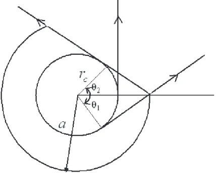
FIG. 3: The representation of rays at the launcher tip.

The radiation is in the interval of angles θ1 < θ < θ2 as shown in Fig. 3 where θ1 =

− arccos¡rc a ¢ and θ2 = arccos ¡_r c a ¢ , respectively, at l = l0 = p a2_{− r}2

c, the field is uniform within the interval θ1 < θ < θ2. We represent this field as a superposition of azimuthal

harmonics,

A0(θ) =

n=∞_X

n=−∞

(10)

The coefficients can be determined as follows. Cn = 1 2π Z _2π 0 A0(θ)einθ = 1 2π einθ2 − einθ1 in (27)

for n 6= 0 and C0 = θ2_2π−θ1. Using Eq. 20, the radiated field, therefore, can be written as

A = n=N_X n=−N Cne−inθe−i n rc(l−l0) w2 ³ n √ αrc − αl 2´ w2 ³ n √ αrc − αl 2 0 ´ · exp µ i2 3α 3/2_(l3 _{− l}3 0) ¶ (28) This is the quasi-optical representation. Using Eq. 25, the asymptotic equation for the radiated field is now written as,

Aasymp= n=N_X n=−N r l0 l Cne −inθ_exp µ −i1 4 n2 α3/2_r2 c µ 1 l − 1 l0 ¶¶ (29) The geometrical optics representation can be expressed as

AGO= n=N_X n=−N r l0 l Cne −inθ_. ₍₃₀₎

Eq. 29 allows us to estimate the Fresnel parameter. At the aperture, the phase varies from 0 to nθ2, where θ2 = arctan

³ l0

rc

´

. Let us assume nθ2 ∼ π. Diffraction occurs if the phase in

the second term varies by the same amount

n2 4α3/2_r2 c µ 1 l − 1 l0 ¶ ∼ π.

From nθ2 ∼ π and the above equation and using Eq. 14 we obtain

4θ2 2 λ

ll0

l − l0 ∼ 1

Introducing the aperture size σ = l0θ2, we obtain the criterion of diffraction

NF = 4σ2 λ µ 1 l − l0 + 1 l0 ¶ ∼ 1,

where NF is a generalized Fresnel parameter. NF À 1 is the region of geometrical optics,

(11)

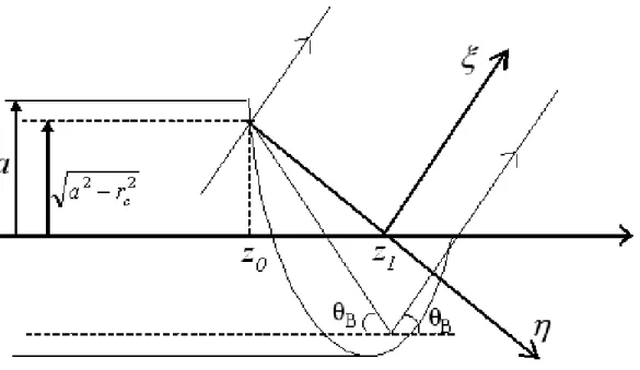
FIG. 4: Ray propagation in the axial plane at the launcher tip.

IV. DIFFRACTION IN AXIAL PLANE

In the previous section, we have considered the radiation from the launcher in the az-imuthal plane. In this section, we consider the axial plane where the geometry of the problem is shown in Fig. 4.

The radiation is coming out at the bounce angle of θB = arcsin ¡_ν

ka ¢

, ν is the root of the equation J0

m(ν) = 0 and a is the waveguide radius. We introduce the coordinates (ξ, η), where ξ is in the direction of propagation and η is in the plane of the phase front.

ξ = (z − z1) cos θB+ y sin θB

η = (z − z1) sin θB− y cos θB

z1 is the coordinate at which the phase front intersects the axis z.

z1 = z0+

p

a2_{− r}2

ctan θB The radiation field is described by the Helmholtz equation,

∂2_u

∂ξ2 +

∂2_u

∂η2 + k

(12)

which we represent in the quasi-optical approximation assuming u = Ae−ikξ_.

−2ik∂A

∂ξ +

∂2_A

∂η2 = 0 (32)

The parabolic equation Eq. 32 has the solution.

A(ξ, η) = Z _∞ −∞ A0(ξ0)G(ξ, η − η0)dη0 (33) where G(ξ, η − η0) = √C ξexp µ −ik(η − η 0₎2 2ξ ¶ (34) is a Green’s function. A0(η) = A(0, η) is the complex amplitude at the plane ξ = 0. The

constant C can be determined from the condition, lim ξ−→0G(ξ, η − η 0_{) = δ(η, η}0_). Therefore C √ ξ Z _∞ −∞ exp µ −ikη 2 2ξ ¶ dη = √C ξ Ã π ik 2ξ !_1/2 = 1 and C = q ik

2π. We assume A0(η) = 1 in the interval η1 < η < η2, where

η1 = − p a2_{− r}2 c sin θB and η2 = − p a2_{− r}2 c cos θB + 4pa2_{− r}2 ccos θB. From Eq. 33 and Eq. 34 we obtain

A(ξ, η) = s ik 2πξ Z _η₂ η1 exp µ −ik(η − η 0₎2 2ξ ¶ dη0 = F Ãs k 2ξ(η2− η) ! − F Ãs k 2ξ(η1− η) ! , (35)

where the Fresnel integral is expressed as

F (x) = r i π Z _x −∞ e−it2 dt (36)

(13)

FIG. 5: Coordinate of the radiation pattern.

V. EXAMPLE OF CALCULATION OF THE LAUNCHER RADIATION

We employ the Surf3D, an electric field integral equation (EFIE) code [12], to propagate the radiation from the launcher to the cylinder which is shown in Fig. 5; (x1, y1) are the coordinates of the observation point. The axis of the cylinder is at the caustic. The launcher radius is a = 2.1966 cm. The caustic radius for the mode TE22,6 is rc= m_νa = 1.059 cm and the transverse wave number is k⊥ = ν_a=20.77 cm−1 where ν is 45.62, which is the 6-th root of the derivative of Bessel function Jm(x) with m=22. Therefore, the angle θ varies from

θ1 = − arccosrc a = −61.2◦ to θ2 = 61.2◦. The parameter α = ³ k⊥ 2r2 c ´_2/3 =4.409 cm−2_{. The} diffraction in the axial plane is calculated for the wave number k=23.05 cm−1 _{at f =110 GHz.}

(14)

l = q r2 1 − 2r1rcsin ϕ1 (37) θ = arccos Ã −r1psin ϕ1− rc l2_{+ r}2 c ! − arccos Ã rc p l2_{+ r}2 c ! (38) The calculations have been carried out for r1=3.3, 4, and 10 cm. Distributions of both

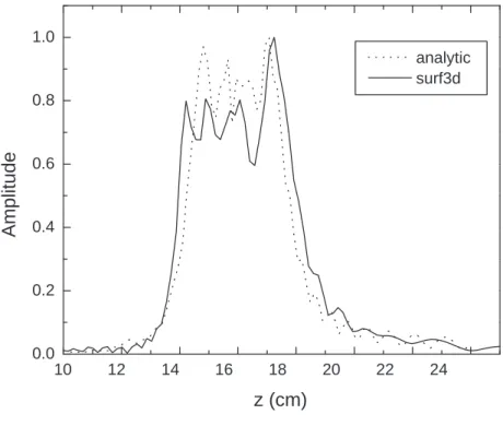
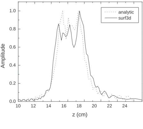
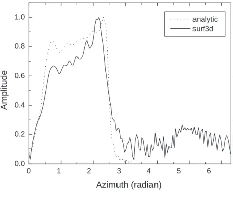
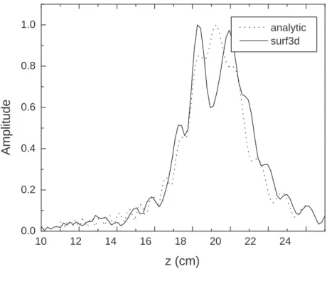
amplitude and phase were calculated using Surf3D and compared to the equation Eq. 28. The number of azimuthal harmonics N in Eq. 28 was chosen to be 18 in the calculation. Fig. 6 through Fig. 11 show the comparison between the Surf3D simulation and analytic solution at the measurement cylindrical plane of radius of 3.3, 4, 10 cm.

We have found very good agreement between the quasi-optical representation of the radiation field and the numerical simulations.

For the field distribution in the axial plane (z axis), the analytic results from the quasi-optical representation are plotted and compared to the numerical results in Figs. 6, 8, and 10. The radiated field patterns from the quasi-optical representation results up to the radius of cylinder of 4 cm match very well with the numerical results for the amplitudes of field and phase. However, as the radius of observation cylinder becomes large (r1=10 cm) there

is a discrepancy at the center of the radiated field between the analytic and numerical results. A better representation is needed to explain the axial field distribution in the far field (Fig. 10(a)).

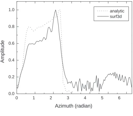
For the field distribution in the azimuthal plane, the results from the quasi-optical rep-resentations (Eq. 29, Eq. 28) are generated and the results show identical field patterns for both representations. This means that once the ray leaves the waveguide it is in the geo-metrical optics zone which extends all the way to infinity. The calculated Fresnel number is

NF = 32 at infinity and larger as we approach to the aperture of the waveguide cut. Only the quasi-optical results are plotted in Fig. 7, 9, and 11 and compared to the numerical results. The amplitude distributions in Figs. 7(a), 9(a), and 11(a) are plotted in the full region of the azimuthal direction which includes the light and dark regions. There is good agreement between the analytic results and numerical results in the light region. The amplitude distri-bution is not symmetrical which is consistent with geometrical optics. In fact, one side on the light region is closer to the aperture than the other. However the sidelobes are present in the amplitude plots in the numerical results whereas the analytic results do not show the sidelobes. The phase distributions presented in Figs. 7(b), 9(b), and 11(b) show also good

(15)

agreement between the analytic theory and the numerical results. The phase flattens out in the light region surrounding the central ray according to the analytic representation. The phase becomes a fast varying function of the azimuthal coordinate outside the light region because the observation cylinder does not coincide with the phase front s = const.

VI. CONCLUSIONS

We have found the quasi-optical solution for the diffraction of the rotating mode at a helical cut of a circular waveguide. Surf3D, a simulation code that solves the electric field integral equation (EFIE) is used to compare the analytic results with numerical simula-tions. The comparison between the Surf3D simulation and analytic solution will give a somewhat better understanding for the mode converter description. The result shows that the quasi-optical representation describes the mode converter well enough for the radiation field qualitatively and to give reasonable quantitative information.

Advanced mode converters utilize an irregular, dimpled waveguide with a helical cut. The results of this calculation can be generalized to represent the radiation from a helical cut of an irregular waveguide. This can be done if the azimuthal amplitude A0(θ) and transverse

amplitude A0(η) are non-uniform.

VII. ACKNOWLEDGEMENT

The authors would like to thank Dr. J. Neilson for providing the Surf3D code. Their research is supported by the U. S. Department of Energy, Office of Fusion Energy Sciences, Washington, D.C.

[1] G. S. Nusinovich, Introduction to the Physics of Gyrotrons. Baltimore: The Johns Hopkins University Press, pp. 87-89 (2004).

[2] M. V. Kartikeyan, E. Borie, M. K. A. Thumm, Gyrotrons, Springer, New Yorker (2004). [3] S. N. Vlasov, L. I. Zagryadskaya, M. I. Petelin, ”Transformation of a whispering gallery mode

propagating in a circular waveguide into a beam of waves,” Radio Eng. Electron. Phys., 20, pp. 14-17 (1975).

(16)

10 12 14 16 18 20 22 24 0.0 0.2 0.4 0.6 0.8 1.0 Amplitude z (cm) analytic surf3d 10 12 14 16 18 20 22 24 -2.0 -1.5 -1.0 -0.5 0.0 0.5 1.0 1.5 2.0 Phase (radian) z (cm) analytic surf3d

(17)

0 1 2 3 4 5 6 0.0 0.2 0.4 0.6 0.8 1.0 Amplitude Azimuth (radian) analytic surf3d 0 1 2 3 4 5 6 -2.0 -1.5 -1.0 -0.5 0.0 0.5 1.0 1.5 2.0 Phase (radian) Azimuth (radian) analytic surf3d

(18)

(19)

(20)

(21)

(22)

[4] M. K. Hornstein, V. S. Bajaj, R. G. Griffin, K. E. Kreischer, I. Mastovsky, M. A. Shapiro, J. R. Sirigiri, R. J. Temkin, ”Second harmonic operation at 460 GHz and broadband continuous frequency tuning of a gyrotron oscillator,” IEEE Trans. Electron Devices, 52, pp. 798-807 (2005).

[5] T. Idehara, I. Ogawa, S. Mitsudo, M. Pereyaslavets, N. Nishida, K. Yoshida, ”Development of frequency tunable medium power gyrotrons (gyrotron FU series) as submillimeter wave radiation sources,” IEEE Trans. Plasma Sci., 27, pp. 340-354 (1999).

[6] J. A. Lorbeck, R. J. Vernon, ”Singly curved dual-reflector synthesis technique applied to a quasi-optical antenna for a gyrotron with a whispering-gallery mode output,” IEEE Trans. Antennas Propag., 39, pp. 1733-1741 (1991).

[7] S. N. Vlasov and M. A. Shapiro, ”Bievolvent mirror for transfer of caustic surfaces,” Sov. Tech. Phys. Lett., 15, pp. 374 (1989).

[8] S. N. Vlasov, M. A. Shapiro, E. V. Sheinina, ”Wave beam shaping on diffraction of a whispering gallery wave at a convex cylindrical surface,” Radio Phys. Quant. Electron., 31, pp. 1070 (1988).

[9] G. G. Denisov, A. N. Kuftin, V. I. Malygin, N. P. Venediktov, D. V. Vinogradov, V. E. Zapevalov, ”110 GHz gyrotron with built-in high efficiency converter,” Int. Journ. Electron., 72, pp. 1079 (1992).

[10] M. Iima, M. Sato, Y. Amano, S. Kobayashi, M. Nakajima, M. Hashimoto, O. Wada, K. Sakamoto, M. Shiho, T. Nagashima, M. Thumm, A. Jacobs, W. Kasparek, ”Measurement of radiation field from an improved efficiency quasi-optical converter for whispering-gallery mode,” Conf. Digest, 14th Int. Conf. on Infrared and Millim. Waves, Wurzburg, Proc. SPIE 1240, pp. 405 (1989).

[11] M. K. Thumm, W. Kasparek, ”Passive high-power microwave components,” IEEE Trans. Plasma Sci., 30, pp. 755-786, (2002).

[12] J. M. Neilson, R. Bunger, ”Surface integral equation analysis of quasi-optical launcher,” IEEE Trans. Plasma Sci., 30, pp. 794 (2002).

[13] H. Shirai, L. B. Felsen, ”Rays and modes for plane wave coupling into a large open-ended circular waveguide,” Wave Motion, 9, pp. 461-482 (1987).

[14] K. Goto, T. Ishihara, L. B. Felsen, ”High-frequency whispering-gallery mode to beam conver-sions on a perfectly conducting concave-convex boundary,” IEEE Trans. Antennas Propag.,

(23)

50, pp. 1109-1119 (2002).

[15] V. A. Fock, ”Electromagnetic diffraction and propagation problems,” Pergamon Press, (1965) [16] G. D. Malyazhinets, L. A. Vainshtein, ”Transverse diffusion for diffraction at an impedance cylinder of large radius. I. Parabolic equation in ray coordinates,” Radiotekh. Elektron., 6, pp. 1247-1258 (1961).

[17] V. M. Babich, V. S. Buldyrev, ”Short-wavelength diffraction theory: asymptotic methods,” Springer-Verlag, (1991).

[18] S. Solimeno, B. Crosignani, P. DiPorto, ”Guiding, diffraction, and confinement of optical radiation,” Acad. Press, (1986).