https://doi.org/10.4224/8913708
READ THESE TERMS AND CONDITIONS CAREFULLY BEFORE USING THIS WEBSITE. https://nrc-publications.canada.ca/eng/copyright
Vous avez des questions? Nous pouvons vous aider. Pour communiquer directement avec un auteur, consultez la première page de la revue dans laquelle son article a été publié afin de trouver ses coordonnées. Si vous n’arrivez pas à les repérer, communiquez avec nous à [email protected].
Questions? Contact the NRC Publications Archive team at
[email protected]. If you wish to email the authors directly, please see the first page of the publication for their contact information.
NRC Publications Archive
Archives des publications du CNRC
For the publisher’s version, please access the DOI link below./ Pour consulter la version de l’éditeur, utilisez le lien DOI ci-dessous.
Access and use of this website and the material on it are subject to the Terms and Conditions set forth at
Mining the Web for Lexical Knowledge to Improve Keyphase
Extraction: Learning from Labeled and Unlabeled Data
Turney, Peter
https://publications-cnrc.canada.ca/fra/droits
L’accès à ce site Web et l’utilisation de son contenu sont assujettis aux conditions présentées dans le site
LISEZ CES CONDITIONS ATTENTIVEMENT AVANT D’UTILISER CE SITE WEB.
NRC Publications Record / Notice d'Archives des publications de CNRC:
https://nrc-publications.canada.ca/eng/view/object/?id=db14b15b-1a02-41f3-8458-f70f9b7108fb https://publications-cnrc.canada.ca/fra/voir/objet/?id=db14b15b-1a02-41f3-8458-f70f9b7108fb
National Research Council Canada Institute for Information Technology Conseil national de recherches Canada Institut de technologie de l’information
Mining the Web for Lexical Knowledge to Improve
Keyphase Extraction: Learning from Labeled and
Unlabeled Data.
*
Turney, P.
July 2002
* published in: NRC/ERB-1096. July 19, 2002. 32 pages. NRC 44947.
Copyright 2002 by
National Research Council of Canada
Permission is granted to quote short excerpts and to reproduce figures and tables from this report, provided that the source of such material is fully acknowledged.
© Copyright 2002 by
National Research Council of Canada
Permission is granted to quote short excerpts and to reproduce figures and tables from this report,
Mining the Web for Lexical Knowledge
to Improve Keyphrase Extraction:
Learning from Labeled and Unlabeled Data
P.D. Turney August 13, 2002 National Research Council Canada Institute for Information Technology Conseil national de recherches Canada Institut de technologie de l’information ERB-1096 NRC-44947
Mining the Web for Lexical Knowledge
to Improve Keyphrase Extraction:
Learning from Labeled and Unlabeled Data
P.D. Turney August 13, 2002
Contents
Abstract ...1 1. Introduction ...1 2. Related Work ...52.1 GenEx: Genitor and Extractor ...5
2.2 Kea: Baseline Feature Set ...6
2.3 Kea: Keyphrase Feature Set ...8
3. Removing Domain-Specificity: Mining for Lexical Knowledge ...9
3.1 A Model of the Keyphrase-Frequency Feature ...9
3.2 PMI-IR: Mining the Web for Synonyms ...10
3.3 Kea: Query Feature Set ...12
4. Experiment 1: Comparison of Feature Sets on the CSTR Corpus ...14
5. Experiment 2: Generalization from CSTR to LANL ...17
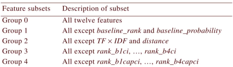
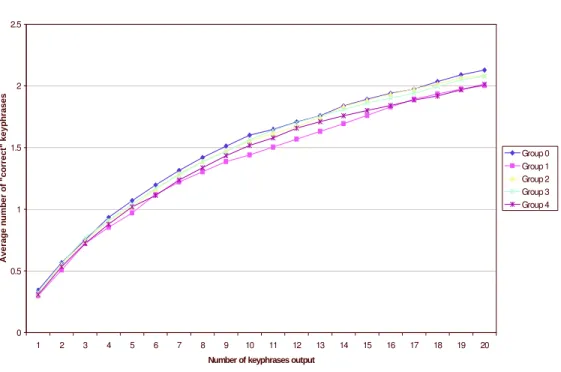
6. Experiment 3: Evaluation of Feature Subsets ...20
7. Experiment 4: Relations Among Feature Sets ...22
8. Experiment 5: Combining Query and Keyphrase Features ...23
9. Experiment 6: Evaluating Keyphrases by Familiarity ...26
10. Experiment 7: Evaluating Keyphrases by Searching ...28
11. Discussion: Limitations, Applications, Future Work ...31
12. Conclusions ...31
Acknowledgments ...32
1. Introduction
Abstract
A journal article is often accompanied by a list of keyphrases, composed of about five to fifteen important words and phrases that capture the article’s main topics. Keyphrases are useful for a variety of purposes, including summarizing, indexing, labeling, categorizing, clustering, high-lighting, browsing, and searching. The task of automatic keyphrase extraction is to select keyphrases from within the text of a given document. Automatic keyphrase extraction makes it feasible to generate keyphrases for the huge number of documents that do not have manually assigned keyphrases. Good performance on this task has been obtained by approaching it as a supervised learning problem. An input document is treated as a set of candidate phrases that must be classified as either keyphrases or non-keyphrases. To classify a candidate phrase as a key-phrase, the most important features (attributes) appear to be the frequency and location of the candidate phrase in the document. Recent work has demonstrated that it is also useful to know the frequency of the candidate phrase as a manually assigned keyphrase for other documents in the same domain as the given document (e.g., the domain of computer science). Unfortunately, this
keyphrase-frequency feature is domain-specific (the learning process must be repeated for each
new domain) and training-intensive (good performance requires a relatively large number of train-ing documents in the given domain, with manually assigned keyphrases). The aim of the work described here is to remove these limitations. In this paper, I introduce new features that are con-ceptually related to keyphrase-frequency and I present experiments that show that the new features result in improved keyphrase extraction, although they are neither domain-specific nor training-intensive. The new features are generated by issuing queries to a Web search engine, based on the candidate phrases in the input document. The feature values are calculated from the number of hits for the queries (the number of matching Web pages). In essence, these new features are derived by mining lexical knowledge from a very large collection of unlabeled data, consisting of approx-imately 350 million Web pages without manually assigned keyphrases.
1.
Introduction
A journal article is often accompanied by a list of keyphrases, composed of about five to fifteen important words and phrases that express the primary topics and themes of the paper. For an individ-ual document, keyphrases can serve as a highly condensed summary, they can supplement or replace the title as a label for the document, or they can be highlighted within the body of the text, to facili-tate speed reading (skimming). For a collection of documents, keyphrases can be used for indexing, categorizing (classifying), clustering, browsing, or searching. Keyphrases are most familiar in the context of journal articles, but many other types of documents could benefit from the use of key-phrases, including Web pages, email messages, news reports, magazine articles, and business papers. The vast majority of documents currently do not have keyphrases. Although the potential benefit is large, it would not be practical to manually assign keyphrases to them. This is the motivation for developing algorithms that can automatically supply keyphrases for a document. There are two gen-eral approaches to this task: keyphrase assignment and keyphrase extraction. Both approaches use supervised machine learning from examples. In both cases, the training examples are documents with manually supplied keyphrases. Otherwise, the two approaches are quite different.
In keyphrase assignment, there is a predefined list of keyphrases (in the terminology of library science, a controlled vocabulary or controlled index terms). These keyphrases are treated as classes, and techniques from text classification (text categorization) are used to learn models for assigning a
1. Introduction
class to a given document (Leung and Kan, 1997; Dumais et al., 1998). A document is converted to a vector of features and machine learning techniques are used to induce a mapping from the feature space to the list of keyphrases. The features are based on the presence or absence of various words or phrases in the input documents. Usually a document may belong to several different classes. That is, a learned model will map an input document to several different controlled vocabulary keyphrases.
In keyphrase extraction, keyphrases are selected from within the body of the input document, without a predefined list. When authors assign keyphrases without a controlled vocabulary (in library science, free text keywords or free index terms), typically about 70% to 80% of their key-phrases appear somewhere in the body of their documents (Turney, 1997, 1999, 2000). This suggests the possibility of using author-assigned free text keyphrases to train a keyphrase extraction system. In this approach, a document is treated as a set of candidate phrases and the task is to classify each candidate phrase as either a keyphrase or non-keyphrase (Turney, 1997, 1999, 2000; Frank et al., 1999; Witten et al., 1999, 2000). A feature vector is calculated for each candidate phrase and machine learning techniques are used to learn a model that can classify a phrase as a keyphrase or non-keyphrase. The features include the frequency and location of the candidate phrase in the input document. The features can also be based on information that is external to the given input docu-ment.
A limitation of keyphrase assignment is that it must be retrained every time a new phrase is added to the controlled vocabulary. Keyphrase extraction does not require retraining, but it can only supply keyphrases that appear somewhere in the input document, unlike keyphrase assignment, which does not have this limitation.
A learning algorithm is training-intensive when it requires a relatively large amount of labeled training examples in order to perform well. Keyphrase assignment is training-intensive when the controlled vocabulary is large, since there must be several training example documents for each key-phrase in the vocabulary. On the other hand, keykey-phrase extraction typically works well with only about 50 training documents (Turney, 1997, 1999, 2000; Frank et al., 1999; Witten et al., 1999, 2000).
A learning algorithm is domain-specific when the learned model does not generalize well from one domain to another domain. Keyphrase assignment is domain-specific, since the appropriate con-trolled vocabulary will vary from one domain to another. For example, the vocabulary of physics articles is distinct from the vocabulary of computer science articles. On the other hand, keyphrase extraction performs well when trained on articles from one domain and then tested on articles from a completely different domain (Turney, 1997, 1999, 2000; Frank et al., 1999; Witten et al., 1999, 2000).
Section 2 discusses prior work on automatic keyphrase extraction. In the GenEx (Turney, 1997, 1999, 2000) and Kea (Frank et al., 1999; Witten et al., 1999, 2000) automatic keyphrase extraction systems, the most important features for classifying a candidate phrase are the frequency and loca-tion of the phrase in the document. There are several versions of Kea, using various methods for finding candidate phrases in a document and various features for classifying the candidate phrases. In one version of Kea, the frequency and location features are supplemented with a feature based on the frequency of the candidate phrase as a manually assigned keyphrase for other documents in the same domain as the given document (Frank et al., 1999). This new feature is called
keyphrase-fre-quency. The experimental results show a significant improvement in keyphrase extraction when the
new feature is added (Frank et al., 1999).
The keyphrase-frequency feature seems to be very useful for keyphrase extraction, but it has two important limitations: it is domain-specific and training-intensive. The training process must be repeated for each new domain and the training process requires a relatively large number of labeled
1. Introduction
training examples to perform well. Suppose that Kea has been trained for the domain of computer science, but now we have a document from the domain of physics. It will not help us to know that a phrase such as “distributed computing” has a high keyphrase-frequency in the domain of computer science. This particular phrase is not likely to be appropriate as a keyphrase for a physics paper. To achieve good performance with physics documents, keyphrase-frequency must be calculated using physics documents (see the experiment in Section 5).
In a sense, when Kea is supplemented with the keyphrase-frequency feature, it becomes a kind of hybrid of the two approaches, keyphrase extraction and keyphrase assignment. The list of phrases for which keyphrase-frequency is non-zero is somewhat like the controlled vocabulary that is used in keyphrase assignment. The problems of domain-specificity and training-intensiveness that come with the new keyphrase-frequency feature are classical problems with the keyphrase assignment approach.
Section 3 introduces new features that are inspired by keyphrase-frequency, yet are neither domain-specific nor training-intensive. These new features exploit the Web as a source of unlabeled data (documents without manually assigned keyphrases). The new features are based on an unsuper-vised learning algorithm called PMI-IR (Turney, 2001, 2002). This algorithm uses Pointwise Mutual Information (PMI) to measure the strength of association between pairs of words. PMI is a statistical measure of word association, based on the frequency of co-occurrence of pairs of words. PMI-IR uses Information Retrieval (IR) to acquire the frequency information that is needed to calculate PMI. The new features are calculated by issuing queries to a Web search engine and analyzing the result-ing number of hits (the number of matchresult-ing Web pages). The queries use the candidate phrases from the input document. In essence, these new features are derived by mining lexical knowledge from a very large collection of unlabeled data, consisting of approximately 350 million Web pages without manually assigned keyphrases.
Beginning with Section 4, the following seven sections present a series of seven experiments. The experiments use the Kea system as a framework for comparing three sets of features: (1) the
baseline feature set is calculated from the frequency and location of the candidate phrases in the
input document, (2) the keyphrase feature set is the baseline feature set supplemented with the
key-phrase-frequency feature, and (3) the query feature set is the baseline feature set supplemented with
features that are calculated using queries to a Web search engine. The first experiment compares the three sets of features on the CSTR corpus (computer science papers from the Computer Science Technical Reports collection of the New Zealand Digital Library Project), when part of this corpus is used for training and the rest is used for testing. In this experiment, the keyphrase features perform best, followed by the query features, and lastly the baseline features. This experiment demonstrates that the query features can improve keyphrase extraction.
In the second experiment (Section 5), part of the CSTR corpus is used for training, but the LANL corpus (physics papers from the arXiv repository at the Los Alamos National Laboratory) is used for testing. In this case, the query features perform best, followed by the baseline features, and finally the keyphrase features. When the training domain does not correspond to the testing domain, the
keyphrase-frequency feature becomes detrimental, instead of beneficial. However, the query features
generalize well from the computer science domain to the physics domain, which shows that they are not domain-specific.
There are a total of twelve features in the query feature set. The third experiment (Section 6) looks at various subsets of the twelve features. The results suggest that all twelve features are useful. Since the query features were inspired by keyphrase-frequency and they are conceptually similar, it was conjectured that the output of Kea with the query feature set would be similar to the output with the keyphrase feature set. The fourth experiment (Section 7) tests this conjecture and finds it to
1. Introduction
be false. The query and baseline features are relatively similar in behaviour, but the keyphrase fea-tures are substantially different from the other two.
This difference suggests that it could be beneficial to combine the query features with the key-phrase features, since they seem to be somewhat independent. The fifth experiment (Section 8) eval-uates a hybrid of the two feature sets. When trained on part of the CSTR corpus and tested on another part of the CSTR corpus, the hybrid feature set performs better than the other feature sets. When trained on the CSTR corpus and tested on the LANL corpus, the performance of the hybrid feature set is very similar to the performance of the keyphrase feature set alone. Thus there is some benefit to combining the features, but the combined feature set has the same limitations as the key-phrase feature set: domain-specificity and training-intensiveness.
The first two experiments measured performance by the number of correct classifications; that is, by the level of agreement between Kea and the author. However, a candidate phrase might be a reasonable, appropriate keyphrase, even though it was not chosen by the author as a keyphrase. One test of reasonableness is whether the phrase was chosen by any author of any paper in the same domain. The sixth experiment (Section 9) repeats the setup of the first two experiments, but mea-sures the performance of the different feature sets by the level of agreement between Kea and the manually assigned keyphrases of any paper in the same testing set. This experiment does not evalu-ate whether the phrases output by Kea are approprievalu-ate for the given input document; it evaluevalu-ates whether the phrases seem reasonable for a paper in the given domain, without regard to the actual content of the paper, beyond its domain. When trained and tested on the CSTR corpus, it is not sur-prising that the keyphrase feature set performs very well by this measure. The difference between the baseline features and the query features is small. When trained on the CSTR corpus and tested on the LANL corpus, the query features perform best, followed by the keyphrase features, and lastly the baseline features.
The seventh and final experiment (Section 10) measures the performance of the keyphrases as query terms for searching. The reasoning is that good keyphrases should be specific enough that they can be used to find the source document, from which they were taken, yet they should be general enough that they can also find many other, related documents from the same domain. This experi-ment compares the keyphrases extracted with the three different feature sets and also the authors’ keyphrases. On the CSTR corpus, there are no significant differences among the baseline, query, and author keyphrases, but the keyphrase-frequency keyphrases are significantly more general than the others. On the LANL corpus, the keyphrase-frequency keyphrases are again the most general. This shows that there is a systematic bias towards generality in the phrases that are chosen when using the
keyphrase-frequency feature.
Section 11 discusses limitations and future work. The main limitation of the new query features is the time that is required to calculate them. Almost all of this time is taken up with network traffic between the machine that runs the learning algorithm and the machine that hosts the Web search engine. However, within ten years, the average desktop personal computer will have enough memory to store 350 million Web pages locally and enough processing power to search them very rapidly.
The main findings of this paper are summarized in Section 12. The new query features improve keyphrase extraction but they are neither domain-specific nor training-intensive. They do require a large amount of unlabeled data, which currently makes them slow to calculate, but improving hard-ware will solve this problem. Although the query features are conceptually related to the
keyphrase-frequency feature, their behaviour is substantially different. In some applications, when the required
training data are available, it may be beneficial to combine the query features with the keyphrase features.
2. Related Work
2.
Related Work
Automatic keyphrase extraction is related to many other technologies, such as automatic summariza-tion (Luhn, 1958; Edmundson, 1969; Kupiec et al., 1995), informasummariza-tion extracsummariza-tion (Soderland and Lehnert, 1994), and keyphrase assignment and automatic indexing (Sparck Jones, 1973; Field, 1975; Leung and Kan, 1997; Dumais et al., 1998). For a general overview of the related literature and the position of keyphrase extraction within this literature, see Turney (2000). The focus here is specifi-cally on prior work in learning to extract keyphrases from text.
2.1 GenEx: Genitor and Extractor
GenEx has two components, the Genitor genetic algorithm (Whitley, 1989) and the Extractor1
key-phrase extraction algorithm (Turney, 1997, 1999, 2000). Extractor takes a document as input and extracts a list of words and phrases as output. The output of Extractor is controlled by a dozen numerical parameters. The setting of these parameters is determined by a training process, during which Genitor searches through the parameter space for values that yield a high overlap between the keyphrases assigned by the authors and the phrases that are output by Extractor. After training, the best parameter values can be hardcoded in Extractor, and Genitor is no longer needed.
To measure the overlap between the machine’s phrases and the author’s phrases, it is necessary to decide when two phrases match. If an author assigns the phrase “Distributed Computation” to a document and the machine extracts the phrase “distributed computing”, this should count as a match. GenEx and Kea both use the same approach for counting matches: phrases are normalized by con-verting them to lower case and stemming them (removing suffixes). Both use the Iterated Lovins stemming algorithm, which applies the Lovins stemming algorithm repeatedly, until the word stops changing (Lovins, 1968; Turney, 1997).
Extractor generates candidate phrases by looking through the input document for any sequence of one, two, or three consecutive words. The consecutive words must not be separated by punctua-tion and must not include any stop words (words such as “the”, “of”, “to”, “and”, “if”, “he”, etc.). Candidate phrases are normalized by converting them to lower case and stemming them.
GenEx has been described in detail elsewhere (Turney, 1999, 2000). In the context of this paper, most of the details of the GenEx algorithm are not important, but it is relevant to know what features are used to select a candidate phrase for output. GenEx does not explicitly represent candidate phrases with feature vectors, but at an abstract level, it may be described as using a set of ten fea-tures (Table 1).
GenEx allows the user to specify the desired number of output phrases. When the user requests N phrases, the ten features are used to calculate a score for every candidate phrase and the top N high-est scoring phrases are output. In the current version of GenEx, N can range from 3 to 30. After a candidate phrase has been selected for output, the final step is to restore the suffix and the original pattern of capitalization.
Experiments show that GenEx performs well when it is trained on one domain and then tested on quite different domains (Turney, 1997, 1999, 2000). Good results are possible with as few as 50 training documents. The level of agreement between the phrases output by GenEx and the phrases assigned by the authors depends on the number of output phrases requested by the user. If the user asks for seven phrases, typically about 20% of the phrases output by GenEx will match the author’s phrases. This is similar to the level of agreement among different humans, assigning keyphrases to
1. Extractor is an Official Mark of the National Research Council of Canada. Patent applications have been submitted for Extractor.
2. Related Work
the same document (Furnas et al., 1987). This figure underestimates the quality of the phrases, since the other 80% of the phrases are often subjectively good, although they do not correspond with the author’s choices. A more accurate picture is obtained by asking human readers to rate the quality of the machine’s output. In a sample of 205 human readers rating keyphrases for 267 Web pages, 62% of the 1,869 phrases output by GenEx were rated as “good”, 18% were rated as “bad”, and 20% were left unrated (Turney, 2000). This suggests that about 80% of the phrases are acceptable (not “bad”) to human readers, which is sufficient for many applications.
Extractor (GenEx without Genitor) has been licensed to 16 companies as a module for embed-ding in products and services. The current version, Extractor 7.2, handles plain text, Web pages, and email messages in English, French, German, Spanish, Japanese, and Korean. It is written in C and has an Application Program Interface (API) to facilitate embedding in other software. Wrappers are available for Perl, Java, Visual Basic, and Python.
2.2 Kea: Baseline Feature Set
Kea generates candidate phrases in much the same manner as Extractor (Frank et al., 1999; Witten et
al., 1999, 2000). Kea then uses the Naïve Bayes algorithm to learn to classify the candidate phrases
(Domingos and Pazzani, 1997). In one version of Kea, candidate phrases are classified using only
two features: TF×IDF and distance (Frank et al., 1999; Witten et al., 1999, 2000). In the following,
I call this the baseline feature set.
TF×IDF (Term Frequency times Inverse Document Frequency) is commonly used in
informa-tion retrieval to assign weights to terms in a document (van Rijsbergen, 1979). This numerical fea-ture assigns a high value to a phrase that is relatively frequent in the input document (the TF
component), yet relatively rare in other documents (the IDF component). In Kea, TF×IDF is
calcu-lated as follows (Frank et al., 1999):
Table 1: Features implicit in GenEx.
Name of feature Description of feature Type of feature
1 num_words_phrase The number of words in the candidate phrase numerical 2 first_occur_phrase The location in the document where the phrase first
occurs
numerical 3 first_occur_word The location in the document of the earliest occurring
word in the phrase
numerical 4 freq_phrase The frequency of the phrase in the document numerical 5 freq_word The frequency of the most frequent word in the phrase numerical 6 relative_length The length of the candidate phrase, relative to other
candidates in the document
numerical
7 document_length The number of words in the document numerical
8 proper_noun Is the phrase a proper noun, based on the capitalization pattern?
boolean 9 final_adjective Is the last word in the phrase an adjective, based on the
suffix?
boolean
10 common_verb Does the phrase contain a common verb, based on a list
of common verbs?
2. Related Work
(1) is the probability that phrase P appears in document D, estimated by counting the number
of times that P occurs in D, , and dividing by the number of words in D, .
is the negative log of the probability that phrase P appears in any document in corpus C,
estimated by counting the number of documents in C that contain P, , and dividing by the
number of documents in C, .
The TF component of TF×IDF in Kea corresponds to the freq_phrase feature in GenEx. In
GenEx, I have found that TF without IDF works well for keyphrase extraction. It is likely that the
relative_length feature in GenEx serves as a surrogate for IDF. Banko et al. (1999) discuss the use of TF×TL as an alternative to TF×IDF, where TL is Term Length (the number of characters in the
term). They argue that TL can replace IDF because longer words tend to have a lower frequency than shorter words. One advantage of TL over IDF is that TL is easier to calculate. Furthermore, TL is
defined for phrases outside of the training corpus C, unlike IDF. In Kea, and are
incremented by one, to avoid taking the logarithm of zero, but TL does not require this kind of adjustment. Also, Kea must assign the same IDF value to all out-of-corpus phrases, but TL only assigns phrases the same value when they are the same length.
The distance feature in Kea is, for a given phrase in a given document, the number of words that precede the first occurrence of the phrase, divided by the number of words in the document. This corresponds to first_occur_phrase in GenEx.
In Kea, a candidate phrase with a capitalization pattern that indicates a proper noun is deleted; it is not considered for output. In GenEx, the document_length feature and the proper_noun feature tend to work together. During training, GenEx tends to learn to avoid proper nouns (phrases for which the proper_noun feature has the value true) for long documents, but allow them for short doc-uments. I conjecture that Kea was mainly developed with a corpus of relatively long documents, for which it is best to suppress proper nouns.
The TF×IDF and distance features are real-valued. Kea uses Fayyad and Irani’s (1993)
algo-rithm to discretize the features. This algoalgo-rithm uses a Minimum Description Length (MDL) tech-nique to partition the features into intervals, such that the entropy of the class is minimized with respect to the intervals and the information required to specify the intervals.
The Naïve Bayes algorithm applies Bayes’ formula to calculate the probability of membership in a class, using the (“naïve”) assumption that the features are statistically independent. Suppose that a
candidate phrase has the feature vector , where T is an interval of the discretized TF×IDF
feature and D is an interval of the discretized distance feature. Using Bayes’ formula and the inde-pendence assumption, we can calculate the probability that the candidate phrase is a keyphrase,
, as follows (Frank et al., 1999):
(2)
In this equation, is the probability that the discretized TF×IDF feature has a value in the
interval T, given that the candidate phrase is actually a keyphrase. is the probability that
the distance feature has a value in the interval D, given that the candidate phrase is actually a
key-phrase. is the prior probability that the candidate phrase is a keyphrase (the probability when
the values T and D are not known). is a normalization factor, to make range
from 0 to 1. is the probability of when the class is not known. These probabilities
can easily be estimated from the frequencies in the training data.
TF P D( , )×IDF P C( , ) freqd(P D, ) sized( )D --- –log2freqc(P C, ) sizec( )C ---× = TF P D( , ) freqd(P D, ) sized( )D IDF P C( , ) freqc(P C, ) sizec( )C freqc(P C, ) sizec( )C T D, p key T D( , )
p key T D( , ) p T key( )⋅p D key( )⋅p key( ) p T D( , ) ---= p T key( ) p D key( ) p key( ) p T D( , ) p key T D( , ) p T D( , ) T D,
2. Related Work
After training, can be used to estimate the probability that a candidate phrase
is a keyphrase. Kea ranks each of the candidate phrases by the estimated probability that they belong to the keyphrase class. If the user requests N phrases, then Kea gives the top N phrases with the highest estimated probability as output.
Experiments comparing GenEx to Kea with the baseline feature set have shown no significant difference in performance (Frank et al., 1999). Other experiments have demonstrated that Kea can improve browsing in a digital library, by automatically generating a keyphrase index (Gutwin et al., 1999), or by automatically generating hypertext links (Jones and Paynter, 1999). The Kea source
code is available under the GNU General Public License.2 The current version, Kea 2.0, is written in
Java. In the following experiments, I used Kea 1.1.4, which is written in a combination of Java, Perl, and C.
2.3 Kea: Keyphrase Feature Set
In another version of Kea, candidate phrases are classified using three features: TF×IDF, distance,
and keyphrase-frequency (Frank et al., 1999). I call this the keyphrase feature set. For a phrase P in a document D with a training corpus C, the keyphrase-frequency is the number of times P occurs as an author-assigned keyphrase in all documents in C that are different from D. Like the other two fea-tures, keyphrase-frequency is discretized using Fayyad and Irani’s (1993) algorithm. Suppose that a
candidate phrase has the feature vector , where T is an interval of the discretized TF×IDF
feature, D is an interval of the discretized distance feature, and K is an interval of the discretized
keyphrase-frequency feature. Using Bayes’ formula and assuming independence, we can calculate as
follows (Frank et al., 1999):
(3) is the probability that the discretized keyphrase-frequency feature has a value in the inter-val K, given that the candidate phrase is actually a keyphrase. These probabilities are easily esti-mated from the training data.
The baseline and keyphrase feature sets have been empirically evaluated using the CSTR corpus (computer science papers from the Computer Science Technical Reports collection in New
Zealand).3 This corpus consists of PostScript files that have been collected from Web sites around
the world. The documents are journal papers, conference papers, technical reports, and preprints in computer science. There is a fair amount of noise in the corpus, because the PostScript files were automatically converted to plain text. For each document in the corpus, the author’s keyphrase list was removed from the title page and placed in a separate file.
In one experiment with the baseline features, the size of the training set was varied from 1 to 130 documents, while the size of the testing set was fixed at 500 documents (Section 2.4.2 in Frank et
al., 1999). The performance measure was the number of machine-extracted keyphrases that matched
the author-assigned keyphrases. The performance on the testing set improved at first, but leveled off after about 50 training documents.
In another experiment, the TF×IDF and distance features were trained on 130 documents and a
separate set of 100 to 1000 documents was used to train the keyphrase-frequency feature (Section 3.2 in Frank et al., 1999). (Since the Naïve Bayes algorithm assumes that features are independent, there
is no difficulty in training the features separately.) The baseline features (TF×IDF and distance)
2. See http://www.nzdl.org/Kea/. 3. See http://www.nzdl.org/. p key T D( , ) T D, p key T D( , ) T D K, ,
p key T D K( , , ) p T key( )⋅p D key( )⋅p K key( )⋅p key( ) p T D K( , , )
---=
3. Removing Domain-Specificity: Mining for Lexical Knowledge
and the keyphrase features (TF×IDF, distance, and keyphrase-frequency) were then evaluated on
the same testing set of 500 documents. The keyphrase feature set performed significantly better than the baseline feature set. The difference in performance rose steadily as the number of documents used to train keyphrase-frequency rose from 100 to 1000. It appears that the performance would have continued to rise with more than 1000 training documents for keyphrase-frequency.
As I mentioned in the introduction, the experiments show that the keyphrase-frequency feature improves keyphrase extraction, but this improvement comes with a cost: domain-specificity and training-intensiveness. The training process must be repeated for each new domain and requires a relatively large number of labeled training examples.
3.
Removing Domain-Specificity: Mining for Lexical Knowledge
This section begins with an analysis of the keyphrase-frequency feature. In the first subsection, I argue that the assumptions underlying the keyphrase-frequency feature imply that keyphrases will tend to co-occur within a domain. This suggests that a statistical measure of co-occurrence might be used to replace the keyphrase-frequency feature. In the second subsection, I introduce a particular statistical measure of co-occurrence, PMI-IR (Turney, 2001). Finally, in the third subsection, I intro-duce a new set of features that are based on PMI-IR.
3.1 A Model of the Keyphrase-Frequency Feature
Consider the following simple model of how the keyphrase-frequency feature works. Suppose we have some documents with associated keyphrases, from the domains of computer science and phys-ics. Let C be the set of all keyphrases that are particularly good for computer science documents and
let P be the set of all keyphrases that are particularly good for physics documents. Let DC be a
prob-ability distribution on C and let DP be a probability distribution on P. Imagine that we assign
key-phrases to a document by deciding whether it is a computer science document or a physics document, and then selecting phrases randomly from the corresponding keyphrase set, C or P, using
the corresponding probability distribution, DC or DP. If this is a reasonable first-order approximation
of how authors assign keyphrases to their documents, then the keyphrase-frequency feature will
work well. The keyphrase-frequency feature is simply an estimate of the probability distribution, DC
or DP, for a given domain, C or P. In fact, if this simple model were completely sufficient to describe
how authors assign keyphrases, then the keyphrase-frequency feature would be the only feature that
worked well; the TF ×IDF and distance features would be irrelevant.
A consequence of this model is that keyphrases will tend to co-occur within a domain. That is, computer science keyphrases will tend to occur together and physics keyphrases will tend to occur together. This is trivially true if C and P have an empty intersection, but it is even true when C and P
are equal, as long as DC and DP are distinct. Suppose that we have a large collection of documents
with associated keyphrases, generated according to our simple model. Let C equal P and let DC and
DP be distinct probability distributions. Suppose that half of the collection consists of computer
sci-ence papers and the other half is physics papers. Let us say that two keyphrases, k1 and k2, tend to
co-occur if the probability that they are both assigned as keyphrases for the same document
is greater than the expected probability , assuming that they are independent.
Let us say that a keyphrase k is a physics keyphrase if it is more probable according to the
distribu-tion DP than according to DC; otherwise, if it is more probable according to DC, we will call it a
computer science keyphrase. We can easily see that k1 and k2 will tend to co-occur if and only if they are both physics keyphrases or both computer science keyphrases. In other words, keyphrases will tend to co-occur within a domain.
3. Removing Domain-Specificity: Mining for Lexical Knowledge
The keyphrase-frequency feature has two limitations. It requires keyphrases to be provided for each document and it requires the domains of the documents to be explicitly identified (in our exam-ple, either physics or computer science). Let us consider an alternative model that does not have
these limitations. Let G be a set of general-purpose phrases (not only keyphrases) and let DG be a
probability distribution on G. Suppose that a document in computer science is generated by
ran-domly sampling phrases from G according to DG and also phrases from C according to DC.
Simi-larly, a document in physics is generated by randomly sampling phrases from G according to DG and
from P according to DP. Now let’s take a document and run it through Kea, using the baseline feature
set. Assume that we do not know whether it’s a computer science document or a physics document.
If the IDF component in the TF×IDF feature is based on a good estimate of DG, and if the DC and
DP distributions are significantly different from DG, then the TF×IDF feature will tend to pick out
phrases from C or P, rather than G, because these phrases will tend to have a higher TF than we
would expect from DG. Thus the phrases that are output by Kea will tend to have a higher density of
phrases from C or P than G, compared to the density in the input document.
This suggests the following two-pass algorithm. In the first pass, we use Kea with the baseline feature set. Then we take the K top ranked phrases output by Kea. If Kea was successful, many of these K phrases are from C or P. By assumption, we do not know whether the input document is a computer science document or a physics document, but we do know that its keyphrases will tend to co-occur. Assume that we are more confident in the quality of the top K phrases than the remaining phrases. In the second pass, we use the top K phrases output by Kea to screen the remaining phrases, by measuring the degree of co-occurrence between the top K phrases and the remaining phrases.
Thus we can exploit co-occurrence information without knowing the domain of the input docu-ment and without knowing the keyphrases that are assigned to the docudocu-ments. Using this two-pass algorithm, we can overcome the two limitations of the keyphrase-frequency feature. The next sub-section presents a measure of co-occurrence and the final subsub-section gives the details of the two-pass algorithm.
3.2 PMI-IR: Mining the Web for Synonyms
PMI-IR uses Pointwise Mutual Information (PMI) and Information Retrieval (IR) to measure the semantic similarity between pairs of words or phrases (Turney, 2001). The algorithm involves issu-ing queries to a search engine (the IR component) and applyissu-ing statistical analysis to the results (the PMI component). The power of the algorithm comes from its ability to exploit a huge collection of text. In the following experiments, I used the AltaVista® search engine, which indexes about 350
million Web pages in English.4
PMI-IR was designed to recognize synonyms. The task of synonym recognition is, given a prob-lem word and a set of alternative words, choose the member from the set of alternative words that is most similar in meaning to the problem word. PMI-IR has been evaluated using 80 synonym recog-nition questions from the Test of English as a Foreign Language (TOEFL) and 50 synonym recogni-tion quesrecogni-tions from a collecrecogni-tion of tests for students of English as a Second Language (ESL). On both tests, PMI-IR scores 74% (Turney, 2001). For comparison, the average score on the 80 TOEFL
4. The AltaVista search engine is a service of the AltaVista Company of Palo Alto, California, http://www.altavista.com/. Including pages in languages other than English, AltaVista indexes more than 350 million Web pages, but these other languages are not relevant for answering questions in English. To estimate the number of English pages indexed by AltaVista, I used the Boolean query “the OR of OR an OR to” in the Advanced Search mode. The resulting number agrees with other published estimates. The primary reason for using AltaVista in the following experiments is the Advanced Search mode, which supports more expressive queries than many of the competing Web search engines.
3. Removing Domain-Specificity: Mining for Lexical Knowledge
questions, for a large sample of applicants to US colleges from non-English speaking countries, was 64.5% (Landauer and Dumais, 1997). Landauer and Dumais (1997) note that, “… we have been told that the average score is adequate for admission to many universities.” Latent Semantic Analysis (LSA), another statistical technique, scores 64.4% on the 80 TOEFL questions (Landauer and
Dumais, 1997).5
PMI-IR is based on co-occurrence (Manning and Schütze, 1999). The core idea is that “a word is characterized by the company it keeps” (Firth, 1957). In essence, it is an algorithm for measuring the strength of associations among words (Turney, 2002).
Consider the following synonym test question, one of the 80 TOEFL questions. Given the prob-lem word levied and the four alternative words imposed, believed, requested, correlated, which of the alternatives is most similar in meaning to the problem word? Let problem represent the problem
word and represent the alternatives. The PMI-IR algorithm assigns
a score to each choice, , and selects the choice that maximizes the score.
The PMI-IR algorithm is based on co-occurrence. There are many different measures of the degree to which two words co-occur (Manning and Schütze, 1999). PMI-IR uses Pointwise Mutual Information (PMI) (Church and Hanks, 1989; Church et al., 1991), as follows:
(4)
Here, is the probability that and co-occur. If and
are statistically independent, then the probability that they co-occur is given by the product . If they are not independent, and they have a tendency to co-occur, then
will be greater than . Therefore the ratio between
and is a measure of the degree of statistical dependence
between and . The log of this ratio is the amount of information that we acquire
about the presence of when we observe . Since the equation is symmetrical, it is
also the amount of information that we acquire about the presence of when we observe
, which explains the term mutual information.6
Since we are looking for the maximum score, we can drop (because it is monotonically
increasing) and (because it has the same value for all choices, for a given problem
word). Thus (4) simplifies to:
(5) In other words, each choice is simply scored by the conditional probability of the problem word,
given the choice word, .
PMI-IR uses Information Retrieval (IR) to calculate the probabilities in (5). For the task of syn-onym recognition (Turney, 2001), I evaluated four different versions of PMI-IR, using four different kinds of queries. Only the first two versions of PMI-IR are needed here. The following description of
these two different methods for calculating (5) uses the AltaVista® Advanced Search query syntax.7
In the following, represents the number of hits (the number of documents retrieved)
given the query .
5. This result for LSA is based on statistical analysis of about 30,000 encyclopedia articles. LSA has not yet been applied to text collections on the scale that can be handled by PMI-IR.
6. For an explanation of the term pointwise mutual information, see Manning and Schütze (1999). 7. See http://doc.altavista.com/adv_search/syntax.html.
choice1,choice2, ,… choicen
{ }
score choice( i)
score choice( i) log2 p problem choice( , i)
p problem( )p choice( i) ---=
p problem choice( , i) problem choicei problem
choicei
p problem( )p choice( i)
p problem choice( , i) p problem( )p choice( i)
p problem choice( , i) p problem( )p choice( i)
problem choicei problem choicei choicei problem log2 p problem( )
score choice( i) p problem choice( , i)
p choice( i) ---= p problem choice( i) hits query( ) query
3. Removing Domain-Specificity: Mining for Lexical Knowledge
1. In the simplest case, we say that two words co-occur when they appear in the same docu-ment:
(6)
We ask the search engine how many documents contain both and , and then
we ask how many documents contain alone. The ratio of these two numbers is the
score for .
2. Instead of asking how many documents contain both and , we can ask how
many documents contain the two words close together:
(7) The AltaVista® NEAR operator constrains the search to documents that contain
and within ten words of one another, in either order.
When the queries yield a sufficient number of hits, tends to perform better than , but
the situation reverses when the queries return only a small number of hits, because
is never larger than .
Table 2 shows how is calculated for the sample TOEFL question, mentioned above. In
this case, imposed has the highest score, so it is (correctly) chosen as the most similar of the alterna-tives for the problem word levied.
3.3 Kea: Query Feature Set
The assumption behind the keyphrase-frequency feature is that documents in the same domain will tend to share keyphrases. In other words, the keyphrases in a given domain (e.g., computer science) will tend to be strongly associated with one another. The shared keyphrases tend to co-occur in the
Table 2: Details of the calculation of score2 for a sample TOEFL question.
Query Hits
imposed 1,198,495
believed 2,537,348
requested 4,774,446
correlated 244,353
levied NEAR imposed 3,593
levied NEAR believed 84
levied NEAR requested 293
levied NEAR correlated 6
Choice Score2
p(levied | imposed) 3,593 / 1,198,495 0.0029979
p(levied | believed) 84 / 2,537,348 0.0000331
p(levied | requested) 293 / 4,774,446 0.0000614
p(levied | correlated) 6 / 244,353 0.0000246
score1(choicei) hits problem AND choice( i)
hits choice( i) ---= problem choicei choicei choicei problem choicei
score2(choicei) hits problem NEAR choice( i)
hits choice( i) ---= problem choicei score2 score1
hits problem NEAR choice( i) hits problem AND choice( i)
3. Removing Domain-Specificity: Mining for Lexical Knowledge
domain. This suggests the following algorithm:
1. For a given document, use the baseline feature set to calculate the probability of
each candidate phrase. Make a list of the top K candidates that have the highest probability of being keyphrases. (In the following experiments, K is 4.) Make another list of the top N candidates that will be further evaluated using the new query features. (We assume N > K. In the following experiments, N is 100. Usually there are many more than 100 candidate phrases, but, for efficiency reasons, we do not re-evaluate all of the candidates. The list of the top N candidates includes the top K candidates.)
2. For each of the top N baseline phrases, use PMI-IR to measure the strength of association with each of the top K baseline phrases. These association strengths will be the new features, the query feature set.
3. For each of the top N baseline phrases, use the new, extended feature set to revise the esti-mated probability that the candidate phrase is a keyphrase. If the user has requested M phrases, then output the top M phrases, according to the revised probability estimate.
The idea is that the top K baseline phrases are the phrases that are most likely to be true keyphrases. Therefore, if a candidate phrase is strongly associated with one or more of the top K baseline phrases, then it is more likely to be a keyphrase.
This is a two-pass algorithm. In the first pass, we run Kea with the baseline feature set. In the second pass, we run Kea with the query feature set. Kea is trained twice with the same training cor-pus. First it is trained with the baseline feature set, then, after the new features have been calculated, it is trained again with the query feature set.
Table 3 lists the twelve features in the query feature set that are calculated in step 2 above. All of the features are numerical. The first four features come from the baseline model. The first two
fea-tures (TF ×IDF and distance) are directly copied from the baseline feature set. The next two
fea-tures (baseline_rank and baseline_probability) are calculated using the baseline model. The four features rank_b1ci, …, rank_b4ci are based on equation (7). For example, rank_b1ci is the score for
the i-th candidate phrase, candidatei, calculated using equation (7) to measure the strength of
associ-ation with the top-ranked baseline phrase, baseline1. The four features rank_b1capci, …,
rank_b4capci are based on equation (6). In these latter four features, the i-th candidate phrase, can-didatei, is transformed to a new phrase, cap_candidatei, by converting the first character of each
word in candidatei to upper case. According to the AltaVista® query syntax, the lower case query
candidatei can match documents that contain the phrase candidatei in any combination of upper and
lower case, but the capitalized query cap_candidatei can only match documents that contain the
phrase candidatei with the same capitalization as cap_candidatei. The hope is that the query
cap_candidatei will only retrieve documents in which the phrase candidatei appears in a title or sec-tion heading. Thus the four features rank_b1capci, …, rank_b4capci are intended to measure the strength of association between the candidate phrases and the top baseline phrases when the candi-date phrases appear in titles or section headings. I use equation (6) (based on “AND”) with the latter four features because the capitalization is likely to reduce the number of hits. On the other hand, I use equation (7) (based on “NEAR”) for the former four features because there are likely to be enough hits.
Features 5 to 12 are normalized as follows. Suppose that is a list of raw values
for one feature. (That is, this is a column from the data table, not a row. There would usually be 100 raw values in this list, rather than just four.) First, the raw values are converted to ranks, where
duplicate raw values map to the same rank. Thus we have , if the raw values are sorted in
descending order. Finally, the ranks are linearly normalized to range from 0 to 1, so we have
p key T D( , )
0.8 0.1 0.3 0.1, , ,
4. Experiment 1: Comparison of Feature Sets on the CSTR Corpus
, if the first rank maps to 1 and the last rank maps to 0. The final normalization ensures that a feature with many duplicate values will span the same range as a feature with few duplicate values. Features are normalized per document, not per corpus. That is, I normalize the fea-tures one document at a time, without regard to any of the other documents. This is a local, contex-tual normalization, as opposed to a global normalization (Turney and Halasz, 1993). As with the other two feature sets, all of the query features are discretized (after normalization) using Fayyad and Irani’s (1993) algorithm. (The discretization is global; it uses the whole training corpus.)
4.
Experiment 1: Comparison of Feature Sets on the CSTR Corpus
This experiment compares the three feature sets using the setup of Frank et al. (1999). The same CSTR corpus is used, with the same training set of 130 documents and the same testing set of 500 documents. Kea 1.1.4 is used as the framework for comparing all three sets of features. The
key-phrase-frequency feature is trained on a separate training set of 1,300 documents.8 The baseline and query feature sets are trained using only the 130 training documents.
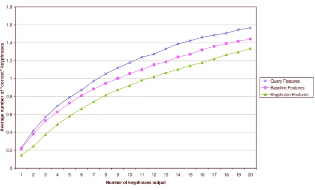
Figure 1 shows the experimental results. The desired number of output phrases varies from 1 to 20. For each requested number of output phrases, the plot shows the average number of output phrases that agree with the authors’ phrases (the “correct” keyphrases). The plot shows that the key-phrase features perform best, followed by the query features, and lastly the baseline features.
Table 3: The query feature set.
Name of feature Description of feature
1 TF×IDF Exactly the same as the baseline TF×IDF feature
2 distance Exactly the same as the baseline distance feature
3 baseline_rank The rank of the candidate phrase in the list of the top N baseline keyphrases 4 baseline_probability The baseline probability estimate p(key | T, D)
5 rank_b1ci The normalized rank of the candidate phrase candidatei when sorted by
hits(baseline1 NEAR candidatei) / hits(candidatei)
6 rank_b2ci The normalized rank of the candidate phrase candidatei when sorted by
hits(baseline2 NEAR candidatei) / hits(candidatei)
7 rank_b3ci The normalized rank of the candidate phrase candidatei when sorted by
hits(baseline3 NEAR candidatei) / hits(candidatei)
8 rank_b4ci The normalized rank of the candidate phrase candidatei when sorted by
hits(baseline4 NEAR candidatei) / hits(candidatei)
9 rank_b1capci The normalized rank of the candidate phrase candidatei when sorted by
hits(baseline1 AND cap_candidatei) / hits(cap_candidatei)
10 rank_b2capci The normalized rank of the candidate phrase candidatei when sorted by
hits(baseline2 AND cap_candidatei) / hits(cap_candidatei)
11 rank_b3capci The normalized rank of the candidate phrase candidatei when sorted by
hits(baseline3 AND cap_candidatei) / hits(cap_candidatei)
12 rank_b4capci The normalized rank of the candidate phrase candidatei when sorted by
hits(baseline4 AND cap_candidatei) / hits(cap_candidatei)
8. I did not perform this training. Kea 1.1.4 is distributed with a pre-trained model for the keyphrase-frequency feature. The 1,300 training documents used to train keyphrase-frequency are from the CSTR corpus.
4. Experiment 1: Comparison of Feature Sets on the CSTR Corpus
Figure 1: Comparison of the three feature sets on the CSTR corpus.
Comparison of Feature Sets on CSTR Test Set
0 0.5 1 1.5 2 2.5 1 2 3 4 5 6 7 8 9 10 11 12 13 14 15 16 17 18 19 20
Number of keyphrases output
A v e ra g e n u m b e r o f " c o rr e c t" k e y p h ra s e s Keyphrase Features Query Features Baseline Features
Figure 2: The difference between the query features and the baseline features.
Difference: Query Features Minus Baseline Features (CSTR Test Set)
0 0.05 0.1 0.15 0.2 0.25 0.3 0.35 1 2 3 4 5 6 7 8 9 10 11 12 13 14 15 16 17 18 19 20
Number of keyphrases output
D if fe re n c e i n a v e ra g e n u m b e r o f " c o rr e c t" k e y p h ra s e s
4. Experiment 1: Comparison of Feature Sets on the CSTR Corpus
Figure 3: The difference between the keyphrase features and the query features.
Difference: Keyphrase Features Minus Query Features (CSTR Test Set)
-0.1 -0.05 0 0.05 0.1 0.15 0.2 0.25 0.3 0.35 1 2 3 4 5 6 7 8 9 10 11 12 13 14 15 16 17 18 19 20
Number of keyphrases output
D if fe re n c e i n a v e ra g e n u m b e r o f " c o rr e c t" k e y p h ra s e s
Keyphrase Minus Query
Difference: Keyphrase Features Minus Baseline Features (CSTR Test Set)
-0.1 0 0.1 0.2 0.3 0.4 0.5 0.6 1 2 3 4 5 6 7 8 9 10 11 12 13 14 15 16 17 18 19 20
Number of keyphrases output
D if fe re n c e i n a v e ra g e n u m b e r o f " c o rr e c t" k e y p h ra s e s
Keyphrase Minus Baseline
5. Experiment 2: Generalization from CSTR to LANL
I used the paired t-test to evaluate the statistical significance of the results (Feelders and Verkoo-ijen, 1995). This is equivalent to applying the Student t-test to the differences between a pair of fea-ture sets. Figure 2 looks at the differences between the query feafea-tures and the baseline feafea-tures. The error bars are 95% confidence regions. The performance of the query features is significantly better than the performance of the baseline features throughout the range of the desired number of output phrases. Figure 3 displays the difference between the keyphrase features and the query features. The performance of the keyphrase features is significantly better than the performance of the query fea-tures when five or more phrases are desired. Finally, Figure 4 plots the difference between the key-phrase features and the baseline features. The performance of the keykey-phrase features is significantly better except when only one phrase is output.
The experiment shows that the query feature set improves on the baseline feature set, although the improvement over the baseline is even larger with the keyphrase feature set. On the other hand, the query feature set does not require the additional 1,300 training documents that are used for the keyphrase feature set. However, the query feature set does use 350 million unlabeled documents.
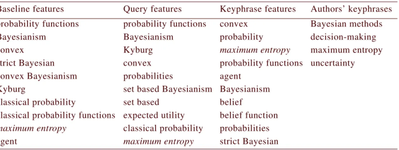
Table 4 gives some examples of the output phrases for the three different feature sets. These are the top ten phrases for a document chosen randomly from the CSTR testing set, entitled, “Set-Based Bayesianism”, by Kyburg and Pittarelli. Matches with the authors are italicized. (These examples are intended to give the reader an impression of the typical output of the algorithms. They are not intended to make any special point.)
5.
Experiment 2: Generalization from CSTR to LANL
This experiment evaluates how well the learned models generalize from one domain to another. The training domain is the CSTR corpus, using exactly the same training setup as in the first experiment. The testing domain consists of 580 documents from the LANL collection (physics papers from the
arXiv repository at the Los Alamos National Laboratory).9 This corpus consists of PostScript files
that have been submitted to the arXiv repository by physicists around the world. The documents are journal papers, conference papers, technical reports, and preprints in physics. There is a fair amount of noise in the corpus, because the PostScript files were automatically converted to plain text. For each document in the corpus, the author’s keyphrase list was removed from the title page and placed
Table 4: Examples of extracted keyphrases and the authors’ keyphrases.
Baseline features Query features Keyphrase features Authors’ keyphrases
probability functions probability functions convex Bayesian methods
Bayesianism Bayesianism probability decision-making
convex Kyburg maximum entropy maximum entropy
strict Bayesian convex probability functions uncertainty
convex Bayesianism probabilities agent
Kyburg set based Bayesianism Bayesianism
classical probability set based belief
classical probability functions expected utility belief function
maximum entropy classical probability probabilities
agent maximum entropy strict Bayesian
5. Experiment 2: Generalization from CSTR to LANL
in a separate file.
Figure 5: Comparison of the three feature sets on the LANL corpus.
Comparison of Feature Sets on LANL Corpus
0 0.2 0.4 0.6 0.8 1 1.2 1.4 1.6 1.8 1 2 3 4 5 6 7 8 9 10 11 12 13 14 15 16 17 18 19 20 Number of keyphrases output
A v e ra g e n u m b e r o f " c o rr e c t" k e y p h ra s e s Query Features Baseline Features Keyphrase Features
Difference: Baseline Features Minus Keyphrase Features (LANL Corpus)
0 0.05 0.1 0.15 0.2 0.25 1 2 3 4 5 6 7 8 9 10 11 12 13 14 15 16 17 18 19 20
Number of keyphrases output
D if fe re n c e i n a v e ra g e n u m b e r o f " c o rr e c t" k e y p h ra s e s
Baseline Minus Keyphrase
5. Experiment 2: Generalization from CSTR to LANL
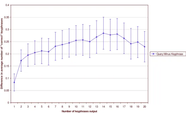
Difference: Query Features Minus Keyphrase Features (LANL Corpus)
0 0.05 0.1 0.15 0.2 0.25 0.3 0.35 0.4 1 2 3 4 5 6 7 8 9 10 11 12 13 14 15 16 17 18 19 20 Number of keyphrases output
D if fe re n c e i n a v e ra g e n u m b e r o f " c o rr e c t" k e y p h ra s e s
Query Minus Keyphrase
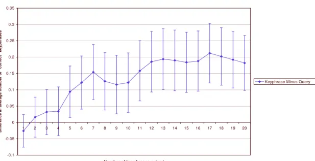
Figure 7: The difference between the query features and the keyphrase features.
D ifference: Q uery F eatures M inus B aseline Features (LANL Corpus)
-0.05 0 0.05 0.1 0.15 0.2 0.25 1 2 3 4 5 6 7 8 9 10 11 12 13 14 15 16 17 18 19 20
Nu m b er o f keyp hrases ou tpu t
D if fe re n c e i n a v e ra g e n u m b e r o f " c o rr e c t" k e y p h ra s e s
Q uery M inus Baseline