Local Ice Pressures from the Louis S. St. Laurent 1994 North Pole Transit

(1)

https://doi.org/10.4224/12340953

Vous avez des questions? Nous pouvons vous aider. Pour communiquer directement avec un auteur, consultez la première page de la revue dans laquelle son article a été publié afin de trouver ses coordonnées. Si vous n’arrivez Questions? Contact the NRC Publications Archive team at

PublicationsArchive-ArchivesPublications@nrc-cnrc.gc.ca. If you wish to email the authors directly, please see the first page of the publication for their contact information.

https://publications-cnrc.canada.ca/fra/droits

L’accès à ce site Web et l’utilisation de son contenu sont assujettis aux conditions présentées dans le site LISEZ CES CONDITIONS ATTENTIVEMENT AVANT D’UTILISER CE SITE WEB.

READ THESE TERMS AND CONDITIONS CAREFULLY BEFORE USING THIS WEBSITE.

https://nrc-publications.canada.ca/eng/copyright

NRC Publications Archive Record / Notice des Archives des publications du CNRC :

https://nrc-publications.canada.ca/eng/view/object/?id=4c65ba5d-55f4-4d67-ad43-6799725a57c7 https://publications-cnrc.canada.ca/fra/voir/objet/?id=4c65ba5d-55f4-4d67-ad43-6799725a57c7

Archives des publications du CNRC

For the publisher’s version, please access the DOI link below./ Pour consulter la version de l’éditeur, utilisez le lien DOI ci-dessous.

Access and use of this website and the material on it are subject to the Terms and Conditions set forth at

Local Ice Pressures from the Louis S. St. Laurent 1994 North Pole Transit

(2)

TP 13671 E

Local Ice Pressures from the Louis S. St. Laurent

1994 North Pole Transit

R. Frederking

Technical Report HYD-TR-054 May 2000

(3)

Local Ice Pressures from the Louis S. St- Laurent 1994 North Pole Transit

R. Frederking

Canadian Hydraulics Centre National Research Council of Canada

Ottawa, Ont. K1A 0R6 Canada

Technical Report HYD-TR-054

(4)

ABSTRACT

Ice pressure data collected from the 1994 Polar transit of the Louis S. St. Laurent were analysed to determine local average ice pressures as a function of size and shape of area of interest as well as the influence of ice thickness and ship

velocity. A probabilistic approach was used to determine annual probability of exceedance of ice pressures. The results indicated a more rapid decrease in pressure with increasing area (exponent –0.7) compared to exponents of –0.4 to –0.5 commonly found in the literature. This is explained on the basis of more frequent loading on smaller hull areas and the definition of area, in this case a

design area. areas In terms of ice thickness at the smallest hull area (0.72 m2) average ice pressure was about 1 MPa higher for ice thicker than 2 m compared to ice thinner than 2m. There was no significant affect of speed on local

pressures for speeds up to 10 kts, however at speeds greater than 10 kts, the average pressure was about 20% greater.

(5)

Local Ice Pressures from the Louis S. St-Laurent 1994

North Pole Transit

1.0 Introduction

Local ice loading is a factor in the design of plating and framing of ships. The pressure-area relation has been used as a means of describing local ice loading. A pattern of decreasing ice pressure with increasing contact area has emerged, sometimes referred to as the pressure-area effect. Daley et al (1985) analysed data from hull instrumentation of the USCGC Polar Sea to determine pressures on a

range of hull areas. The 9-m2 instrumented area was comprised of 60 elements,

each 0.15 m2 in area, and a trend of higher pressures for smaller areas was

observed. Masterson and Frederking (1993) collected data in the context of local ice loads, covering areas ranging from 10-1 m2 to 102 m2 and also defined a trend of decreasing pressure with increasing contact area.

Two fundamentally different types of pressure-area relations are identified from these reported data. One describes the change in average ice pressure as a function of contact area during an impact, such as a ship ramming a large ice feature (Riska, 1987). This can be termed a process pressure-area relation. The other pressure-area relation describes the average pressure on sub-areas of various sizes within a larger contact area at an instant in time during an impact. This is the type of pressure-area relation presented by Daley et al (1985) and referred to by Jordaan et al (1993) as pressure on local areas within a global area. This situation can be termed as describing a spatial distribution pressure-area relation.

Transport Canada has supported R&D to aid development of a Code for

Polar Navigation in concert with other national administrations for eventual

promulgation by the International Maritime Organisation (I.M.O.) (see Santos-Pedro, 1994). This included full-scale field trials, laboratory experiments, model tests and analytical model development by Canadian and other researchers.

Recently the Louis S. St. Laurent was instrumented to measure hull response to ice loads (Ritch et al, 1999). The instrumented area was of the order

of 20 m2 and local loads over 30 elements within this area were measured. The

areas were large enough and the number of elements sufficient that information on the nature of the ice contact area and the pressure distribution within it could be determined. This report will examine the time series data of local ice loading from the 1994 Polar transit of the Louis S. St. Laurent. The data provide the opportunity to determine the average pressures on various sizes and shapes of

(7)

hull areas from a probabilistic perspective. Note, however, that the analysis of this report does not directly address the issue of contours of pressure within the contact area.

2.0 Voyage Details

The voyage involved the Louis S. St. Laurent and the US Coast Guard Cutter Polar Sea. The vessels transited from Alaska (Chukchi Sea) across the Pole to Svalbard (Fram Strait). The ice edge was encountered on July 26, 1994 at

70o08’N, 168o38’W and the North Pole reached on August 22. The ships left the

ice on August 30 at about 80oN, 14oE. The distance from the ice edge to the

Pole was 1420 n-mile and the total voyage distance in ice 2120 n-miles. The average speed while underway from the ice edge to the North Pole was 3.68 kt (Ritch et al 1999). The total voyage in ice lasted 35 days, but the actual time the ships were transiting was about 500 hours. The difference is due to time while the ships were stopped to recover oceanographic and ice samples, ceremonies at the North Pole, and delays encountered due to propeller damage to the Polar Sea. The cumulative distance and speed, as determined from hourly observations from the Polar Sea are plotted in Figure 1 and 2. The cumulative distance plot shows the relatively steady progress in reaching the North Pole (August 22) followed by more rapid progress towards exiting the ice near Svalbard. The speed plot in Figure 2 shows that the vessels operated at a wide range of speeds throughout the voyage.

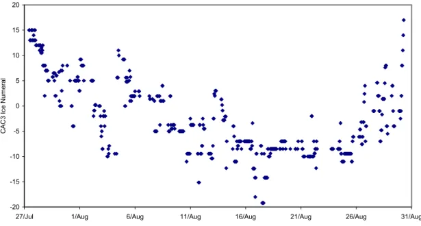
Hourly observations of ice conditions were taken from the bridge of the Polar Sea. These included ice classification by type, thickness, ridging and partial concentrations by ice type. It was possible to calculate an Ice Numeral from the ice observations. Assuming a CAC3 class for the vessels the calculated Ice Numerals are plotted in Figure 3. Ice Numerals decreased as the Pole was approached, and were substantially negative for a significant part of the voyage. Video records from over the side and bridge mounted cameras were made on the Louis S. St. Laurent. These videos were later used to verify ice thickness and ice conditions during the voyage.

3.0 Instrumentation

Three areas on the Louis S. St. Laurent were instrumented to measure ice loads: the bow, shoulder and bottom. This report focuses on the bow area. An area 7.2-m long by 3 m high just below the water line, and approximately midway between the stem and the shoulder, was instrumented. The top of this area was about 0.75 m below the waterline. Six main frames were instrumented with strain gauges to measure the shear strain difference between two stingers spaced 3 m apart vertically. The general layout is illustrated in Figure 4. For the forward frame

(8)

(229) and the two aft frames, only the top and bottom were strain gauged so the total force over a 3 m height of the frame was determined. However, for each of the middle three frames (shown shaded in Figure 4) four additional gauges were equally spaced so that loads over five 600-mm-high sub-panels could be determined. An extrapolation routine was used to generate sub-panel loads for the frames that only had strain gauges at the top and bottom (Ritch et al, 1999). Consequently average pressures on an array of 30 panels, where each

sub-panel was 1.2 m wide by 0.6 m high (area 0.72 m2) were available for analysis. By

summing the output of two, four, six or eight immediately adjacent panels,

average pressures on areas larger than 0.72 m2 could also be obtained.

Summing all 30 sub-panels provided a good representation of the total ice load on the portion of the bow that was instrumented. Impacts on the other side of the bow or outside the instrumented area were not recorded.

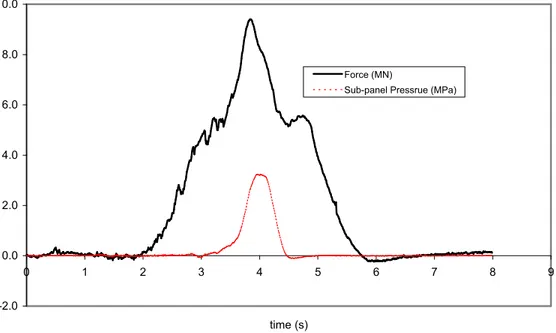
Records were saved whenever a threshold strain was exceeded, in this case 200 µm/m, well within the elastic limit of steel. The scan rate was 100 Hz and the record length has 6 to 10 seconds. Part of the record prior to the trigger was stored, so a time series record of the total event, from start of loading to unloading, was obtained. As an example, a time series record of the total load on the instrumented area and the average ice pressures on one sub-panel at level C (see Figure 4) is presented in Figure 5 for an impact event while the ship was traveling at 4 m/s in ice 1 to 2 m thick ice. In this case the maximum load on the instrumented area is 9.5 MN and the maximum pressure is about 3 MPa for the sub-panel examined. As mentioned above, the ice pressure on a pair of adjacent sub-panels can be averaged to obtain a time series record of average pressure on a larger area. Figure 6 is a time series plot of the average ice pressure on the single sub-panel presented in Figure 5 and the average pressure

on it plus one adjacent sub-panel (area 1.44 m2). It can be seen that for the

impact event the maximum pressure on the single sub-panel was 3.2 MPa and on the two sub-panels was 2.3 MPa, and that the maximums did not occur at the same time. In a similar manner, time series records of average ice pressure on various sizes and shapes of areas can be determined and a maximum pressure for the event determined. Thus for each event a maximum pressure on a selection of sizes and shapes of hull area can be determined.

Figure 7 illustrates the areas and shapes of area identified for analysis. The shaded area was swept across the instrumented sub-panels at each time step to determine the largest average pressure on the predetermined area during an event. This area, which is termed a design area here, is different from the contact area between the ice and hull. The actual area of contact, even at the instant of maximum average pressure, may in some cases be less than the design area, and for large areas this is definitely the case. Table 1 illustrates the characteristics of each of the areas identified in Figure 7. The aspect ratio is the ratio of the width to the height of the area. The number of areas is the number of locations that the selected area can be placed on the instrumented area.

(9)

Table 1 Sample areas used for analysis of average local ice pressures

Figure 7 illustration Area (m2) Aspect Ratio Number of areas

(a) 0.72 2:1 30 (b) 1.44 4:1 25 (b) 2.88 2:1 20 (d) 5.76 4:1 12 (e) 6.48 2:1 12 (f) 11.52 2:1 6 (g) 1.44 1:1 24 (h) 2.88 1:2 12 (i) 5.76 1:1 10 (j) 12.96 4:1 3 Whole area 21.6 2.4:1 1

4.0 Analysis of Impact Events

During the voyage 1730 bow impact events were recorded on the Louis S. St. Laurent. Using the procedure outlined in Section 3, a set of independent extreme values of average ice pressure was obtained for each of the eleven areas and shapes for each event. The extreme values for all the events were arranged in descending order and plotted using the following plotting position

pe = i/(n+1) (1)

where i is the ith ranked data point and n is the total number of data points. The

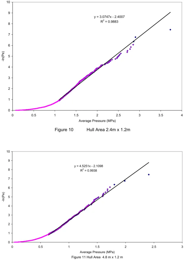
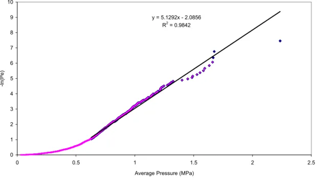
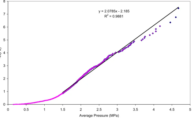
ranked load data were plotted versus –ln(pe ). Plots for each of the eleven cases

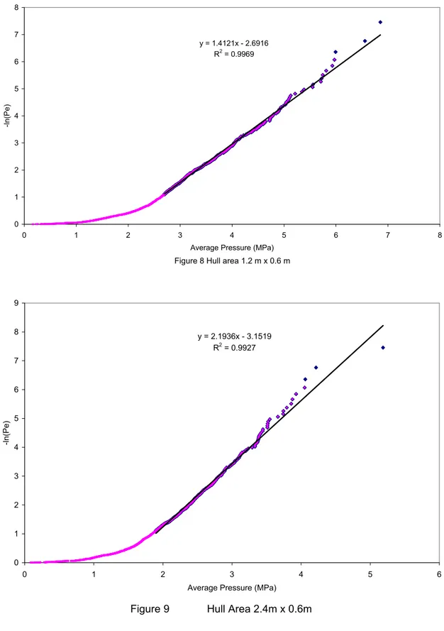
analysed are presented in Figures 8 to 18. Disregarding the lower load data, a single exponential expression can be fit to the higher pressure results. Straight-line curves were fit to the higher pressure data using least squares. The best-fit line and the equation ( y = mx + b ) describing it are shown on each figure. The following expression describes the best fit line

pe = exp[-(x-xo)/α] (2)

where y = -ln(pe), xo is the intercept with the x-axis and α is the inverse of the

slope of the line (m). The results of the fits to the higher data in Figures 8 to 18 are summarized in Table 2 below.

Table 2 Summary of fits to local pressure distributions

(10)

(m2) Ratio for fit (MPa) (1/MPa) (m) intercept (b) 0.72 2:1 2.7 1.41 -2.69 1.44 4:1 1.9 2.19 -3.15 2.88 2:1 1.1 3.07 -2.40 5.76 4:1 0.64 4.53 -2.11 6.48 2:1 0.63 5.13 -2.09 11.52 2:1 0.4 7.88 -2.02 1.44 1:1 1.5 2.08 -2.18 2.88 1:2 1.1 3.15 -1.38 5.76 1:1 0.8 4.35 -1.34 12.96 4:1 0.35 8.35 -1.80 21.6 2.4:1 0.2 12.45 -1.65

Exposure has to be taken into account before these data can be used to make estimates of extreme loads. The first aspect of exposure relates to the number of sub-panels in the areas used in the data compilation. In the case of a single sub-panel, pressures on 30 sub-panels were measured. The probability of any one of these sub-panels experiencing a maximum pressure is less than that for the 30 sub-panels. The probability is thus reduced by ln(30), or 3.4. Similarly, adjustments are made for the two, four, eight and so on sub-panel groups. The other aspect of exposure is the number of events or peak loads in a given time period or distance traveled. The ship can be assumed to be a device for measuring local ice pressures, however, the actual pressures measured are possibly a function of ice thickness and ship speed. A ship with lesser capabilities than the Louis S. St. Laurent would probably be handled in a manner which would result in lower ice impact pressures or fewer impact events. At this point, for the sake of argument, it will be assumed that time will be the measure of exposure. Over the 500 hours of transit, 1730 impacts were recorded on the bow, or a rate of 3.5 events per hour of transit in polar ice. A ship such as the Louis S. St. Laurent might be expected to be under transit about 1000 hours annually, and thus the number of events expected annually is 3500. The Memorial University review (Carter et al, 1992) of the Arctic Shipping Pollution Prevention Regulations suggested that a ship like the Louis S. St. Laurent could expect to encounter of the order of 100 rams with multi-year ice each year. Not all the impacts in the 1994 Polar transit were with multi-year ice, nor could they be described as ramming, so considerable judgement is needed in establishing an appropriate exposure. It should also be said that other ships having different mission profiles might expect more or fewer events annually.

Jordaan et al (1993) suggested the following approach to establishing the load level corresponding to a particular annual exceedance value. The extreme annual load Z is given by

(11)

where there are N events Xi in the year. The distribution of the maximum of Z is

given by

FZ(z) = exp{-exp[-(z-xo-x1)/α]} (4)

where x1 = Χ ln n. This equation can be re-arranged to give the extreme load ze

corresponding to a given exceedance probability, [1-FZ(ze)], by the following

expression

ze = xo + α{-ln[-ln(1- FZ(ze))] + ln(n)} (5)

A 1% annual exceedance is a reasonable limit to select for local pressures which, if exceeded, would result in denting, but not failure or breaching of the

hull. For 1% annual exceedance, -ln[-ln(1- FZ(ze))] = 4.6 and equation (5)

becomes

z0.01 = xo + α{4.6 + ln(n)} (6)

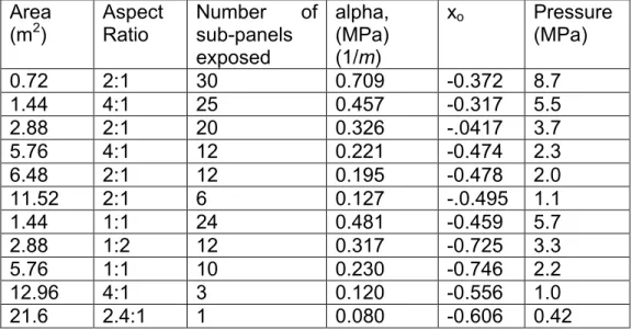
As discussed above, the annual number of events is taken to be 3500, hence this number would be substituted for n. The results of these calculations are summarized in Table 3.

Table 3 Predicted local pressures for 1% annual exceedance (3500 events) Area (m2) Aspect Ratio Number of sub-panels exposed alpha, (MPa) (1/m) xo Pressure (MPa) 0.72 2:1 30 0.709 -0.372 8.7 1.44 4:1 25 0.457 -0.317 5.5 2.88 2:1 20 0.326 -.0417 3.7 5.76 4:1 12 0.221 -0.474 2.3 6.48 2:1 12 0.195 -0.478 2.0 11.52 2:1 6 0.127 -.0.495 1.1 1.44 1:1 24 0.481 -0.459 5.7 2.88 1:2 12 0.317 -0.725 3.3 5.76 1:1 10 0.230 -0.746 2.2 12.96 4:1 3 0.120 -0.556 1.0 21.6 2.4:1 1 0.080 -0.606 0.42

These results for local pressure on various sizes and shapes of hull area are plotted in Figure 19. A best-fit line through the results of the four areas with aspect ratio 2:1 is given by the following power relation

(12)

p = 7.3 A –0.7, for 0.72 m2 < A < 10 m2 (7)

where p is the average local pressure in MPa, and A is the area in m2. the area

in Figure 19 is the design area discussed in Section 3. Results for other aspect ratios are also plotted in Figure 19, but it can be seen that there is little affect of aspect ratio within the observed range (4:1 to 1:2). The exponent on the average pressure, -0.7 is less that the values recorded in the literature (-0.4 to –0.5), see for example Masterson and Frederking (1993) or Riska (1987). Equation (7) also takes into account exposure, in that there will be more loadings on small hull areas than large areas. If all hull areas were treated as having equal exposure the exponent on Equation (7) would be smaller. To illustrate this point, if the maximum average pressures from Figures 8, 10, 12 and 13 were used, disregarding exposure, the following pressure area relation would be determined

p = 5.8 A –0.56, for 0.72 m2 < A < 10 m2 (8)

It is interesting to note that the exponent of –0.7 is the same as that reported by Jordaan et al (1993) for analysis of local ice pressures on the Polar Sea and the Canmar Kigoriak. .

The data in Table 3 also provide an opportunity for examining the effect of

shape of the loaded area. For an area of 1.44 m2, the average pressure for

aspect rations 4:1 and 1:1 5.5 MPa and 5.7 MPa respectively, and at 5.76 m2,

2.3 MPa and 2.2 MPa respectively. This supports the contention that within this range of areas and aspect ratios, aspect ration is not a factor in determining average pressure. Aspect ratios ranging from 4:1 to 1:2 were examined, but no clear trend emerged. Note that Ritch et al (1999), in analysing the same data set established that actual aspect ratios were in the range 3:1 to 1:1, and again no trends were apparent in that range.

The preceding analysis was for 1000 hours of annual transit exposure. For more or fewer hours of annual exposure, the coefficient on the above pressure-area relation (Eqn. 7) would be adjusted upwards or downwards.

5.0 Effect of Ice Thickness and Ship Speed on Impact

The analysis of the previous section included all impact events, which covered a range of ice thickness from 1.2 m to 7.6 m and speeds from 0.4 to 16 knots. There is a question as to whether ice thickness or ship speed affect local ice pressures. To examine this question the data have been reviewed in terms of ice thickness and impact speed. The impact events were sorted in terms of thickness and speed. Thickness categories of 1 to 2 m, 2 to 3 m and greater than 3 m were selected. Following a similar procedure to that outlined in Section

(13)

4, the local ice pressures for each thickness category were arranged in descending order and plotted against the plotting position defined in Equation (1). The results are plotted in Figure 20 for a single sub-panel 1.2 m wide by 0.6 m high. The average pressure for ice thickness 2 to 3 m and greater than 3 m are virtually identical, but pressures are about 1 MPa lower for thinner ice, 1 to 2 m thickness. The average pressure over the entire 3.0 by 7.2 m area is plotted in Figure 21. Here there is a progressive trend of increasing pressure with each thickness category. For ship speed effect, four categories were established, 0-3 m/s, 3-6 m/s, 6-10 m/s and > 10 m/s. In Figures 22 and 23 the distributions of average pressure for each speed category on a single sub-panel and the whole instrumented area, respectively, are plotted. No systematic effect of speed can be seen for speeds up to 10 m/s. However, once speed exceeded 10 m/s, higher average pressures are observed.

6.0 Comparisons

The local pressure data measured on the bow of the Louis S. St. Laurent provide a good basis for examining local ice pressures. The local pressure-area relation with a 1% annual probability of exceedance, assuming 1000 hours of transit (3500 impact events) was found to be

p = 7.3 A –0.7, for 0.72 m2 < A < 10 m2 (9)

The area in Equation 7 is a design area, as discussed in Section 3. By way of comparison, Masterson and Frederking (1993) proposed the following relation as a “normal design curve”:

p = 8.1 A –0.5, for 0.1 m2 < A < 29 m2 (10)

The probability of exceedance of this design curve was 5%. It was derived from over 500 data points from a broad range of sources. Area in this case is a nominal contact area based on the geometry of indentation. Ritch et al (1999), analysing the 1994 Louis S. St. Laurent data, identified a “pressure asymptote” line

p = 5.9 A –0.4, for 0.67 m2 < A < 8 m2 (11)

as an upper bound of the pressure measurements during impact. The area here is a loaded or actual contact area. Note that the area in the case of Equation (11) does not take into account exposure on smaller areas. For easier comparison these three equations are plotted in Figure 24. It can be seen that the results of the analysis in this report indicate that the average pressure decreases more rapidly with increasing area than the other two equations.

(14)

However, three different definitions of area have been used in the three cases, so some of the difference may be due to definition.

A previous analysis of Canmar Kigoriak and USCG Polar Sea data (Jordaan, 1992) resulted in a pressure area relation in which the coefficient on the area was –0.7m, identical to the value determined in this study.

7.0 Conclusions

The local pressure data collected from the 1994 Polar transit of the Louis S. St. Laurent provide a good basis for examining local ice pressures which could be expected by ships transiting ice covered waters. There are a sufficient number of events to allow a probabilistic examination of local ice pressures as a function of size and shape of hull area as well as the influence of ice thickness and ship velocity. The analysis in this report indicates a more rapid decrease in pressure with increasing area (exponent –0.7) compared to exponents of –0.4 to –0.5 commonly found in the literature. This exponent of -0.7 is a result exposure (more frequent loading on smaller areas) and the definition of area in this study as a design area. In any application of a local pressure area relation, care must be taken to account for exposure and the definition of area. Also the relation should not be extrapolated to areas larger than those for which data are available.

No influence on average pressure was observed for the shape of the hull area, for aspect ratios (width:height) 4:1 to 1:1.

Some effect of ice thickness and ship speed was observed. For the smallest

area (0.72 m2), average ice pressure was about 1 MPa greater for ice thickness

of 2 to 3 m, but no further increase was observed for ice thicker than 3 m. For

the largest (21 m2) area, there was a systematic increase in average pressure

with increasing ice thickness. The influence of ship speed on average pressure was less clear. For both the smallest and largest areas, there was no significant effect of speed for speeds up to 10 kt, however at speeds greater than 10 kt, the average pressure was greater than for lower speeds

8.0 References

Carter, J.E., Frederking, R., Jordaan, I.J., Milne, W.J. and Nessim, M.A., 1992. Review and verification of proposals for revisions of the Arctic Shipping Pollution Prevention Regulations – final report, Memorial University of

Newfoundland, Ocean Engineering Researchj Centre, St. John’s, (TP11366E). Daley, C., St. John, J.W., Seibold, F, and Bayly, I. 1985. Analysis of extreme ice

loads and pressures on USCGC Polar Sea, SNAME Annual Meeting, November 1984, Paper No. 8

(15)

Jordaan, I.J., Maes, M.A., Brown, P.A. and Hermans, I.P. 1993. Probabilistic analysis of local ice pressures, Journal of Offshore and Arctic Engineering, ASME Vol. 115, pp. 83-89.

Masterson, D.M. and Frederking, R. 1993. Local contact pressures in ship/ice and structure/ice interactions, Cold Regions Science and Technology, Vol. 21, pp. 169-185.

Ritch, R., St. John, J., Browne, R., and Sheinberg, R., 1999. Ice load impact measurements on the CCGS Louis S. St. Laurent during the 1994 Arctic

Ocean crossing, Proceedings of the 18th International Conference on

Offshore Mechanics and Arctic Engineering, July 11-16, 1999, St. John’s Newfoundland, paper OMAE99/P&A-1141.

Riska, K., 1987. On the mechanics of the ramming interaction between a ship and a massive ice floe, Thesis for degree of Doctor of Technology, Technical Research Centre of Finland, Publication 43, Espoo, Finland.

Santos-Pedro, V.M., 1994. The case for harmonization of (polar) ship rules, SNAME, Icetech ’94 Proceedings, Calgary, March 1994, paper D.

(16)

Figure 1 Accumulated distance transited by Polar Sea 1994 0 500 1000 1500 2000 2500

27/Jul 1/Aug 6/Aug 11/Aug 16/Aug 21/Aug 26/Aug 31/Aug

accumulated distance (n-mi)

North Pole

Figure 2 Speed at hourly intervals - Polar Sea 1994

0 2 4 6 8 10 12 14

(17)

Figure 3 ASPPR Ice Numerals calculated for Polar Sea as CAC3 -20 -15 -10 -5 0 5 10 15 20

CAC3 Ice Numeral

Frame 229 A B C D E FORWARD AFT Frame 226 Frame 223 Frame 220 Frame 217 Frame 214 3.0 m 0.7 m 7.2 m

(18)

Figure 5 Total force on bow area and average pressure on one sub-panel, impact at 4 m/s on 1-2 m thick ice

-2.0 0.0 2.0 4.0 6.0 8.0 10.0 0 1 2 3 4 5 6 7 8 9 time (s) Force (MN)

Sub-panel Pressrue (MPa)

Figure 6 Comparison of average pressures on one and two sub-panels, for 4 m/s impact on 1-2 m thick ice -0.5 0 0.5 1 1.5 2 2.5 3 3.5 0 1 2 3 4 5 6 7 8 time (s)

average pressure (MPa)

1 sub-panel 2 sub-panels

(19)

(a) 229 226 223 220 217 214 (f) 229 226 223 220 217 214 A 0.72 A 11.5 B 2:1 B 2:1 C C D D E E (b) 229 226 223 220 217 214 (g) 229 226 223 220 217 214 A 1.44 A 1.44 B 4:1 B 1:1 C C D D E E (c) 229 226 223 220 217 214 (h) 229 226 223 220 217 214 A 2.88 A 2.88 B 2:1 B 1:2 C C D D E E (d) 229 226 223 220 217 214 -1 229 226 223 220 217 214 A 5.76 A 5.76 B 4:1 B 1:1 C C D D E E (e) 229 226 223 220 217 214 (j) 229 226 223 220 217 214 A 6.48 A 13 B 2:1 B C C D D E E

(20)

Figure 8 Hull area 1.2 m x 0.6 m y = 1.4121x - 2.6916 R2 = 0.9969 0 1 2 3 4 5 6 7 8 0 1 2 3 4 5 6 7 8

Average Pressure (MPa)

-ln(Pe)

Figure 9 Hull Area 2.4m x 0.6m

y = 2.1936x - 3.1519 R2 = 0.9927 0 1 2 3 4 5 6 7 8 9 0 1 2 3 4 5 6

(21)

Figure 10 Hull Area 2.4m x 1.2m

Figure 11 Hull Area 4.8 m x 1.2 m

y = 4.5251x - 2.1098 R2 = 0.9938 0 1 2 3 4 5 6 7 8 9 10 0 0.5 1 1.5 2 2.5 3

-ln(Pe) y = 3.0747x - 2.4007 R2 = 0.9883 0 1 2 3 4 5 6 7 8 9 10 0 0.5 1 1.5 2 2.5 3 3.5 4

(22)

Figure 12 Hull Area 3.6 m x 1.8 m y = 5.1292x - 2.0856 R2_{= 0.9842} 0 1 2 3 4 5 6 7 8 9 10 0 0.5 1 1.5 2 2.5

-ln(Pe)

y = 7.876x - 2.024 R2 = 0.9949 0 1 2 3 4 5 6 7 8 9 10 0 0.2 0.4 0.6 0.8 1 1.2 1.4 1.6

(23)

Figure 14 Hull Area 1.2 m x 1.2 m y = 2.0785x - 2.185 R2 = 0.9881 0 1 2 3 4 5 6 7 8 0 0.5 1 1.5 2 2.5 3 3.5 4 4.5 5

-ln(Pe)

y = 3.1522x - 1.3769 R2 = 0.9854 0 1 2 3 4 5 6 7 8 9 0 0.5 1 1.5 2 2.5 3 3.5

(24)

Figure 16 Hull Area 2.4 m x 2.4 m y = 4.3499x - 1.3359 R2 = 0.9833 0 1 2 3 4 5 6 7 8 9 0 0.5 1 1.5 2 2.5

-ln(Pe)

y = 8.3496x - 1.7974 R2 = 0.9967 0 1 2 3 4 5 6 7 8 0 0.2 0.4 0.6 0.8 1 1.2

(25)

Figure 18 Hull Area 7.2 m x 3.0 m y = 12.453x - 1.6468 R2 = 0.9949 0 1 2 3 4 5 6 7 8 9 0 0.1 0.2 0.3 0.4 0.5 0.6 0.7 0.8

-ln(Pe)

Figure 19 Average Pressure as a function of hull area y = 7.2845x-0.7236 R2 = 0.9879 0.1 1 10 0.1 1 10 100 Area (m^2) Pressure (MPa) Aspect Ratio 2:1 Aspect Ratio 4:1 Aspect ratio < 1:1 Bow Panel Aspect Ratio 2:1

(26)

Figure 20 Ice Thickness effect on sub-panel pressure y = 1.5478x - 2.2748 R2 = 0.9936 y = 1.3056x - 2.2096 R2 = 0.9648 y = 1.3983x - 2.7944 R2 = 0.9957 0 1 2 3 4 5 6 7 8 0 1 2 3 4 5 6 7 8

average pressure on 1.2x0.6 m (MPa)

-ln(Pe)

1-2 m 2 - 3 m > 3 m

Figure 21 Ice thickness effect on total instrumented area pressure y = 23.048x - 4.4107 R2_{= 0.9858} y = 14.218x - 2.0619 R2_{= 0.9629} y = 11.739x - 1.5394 R2 = 0.9955 0 1 2 3 4 5 6 7 8 0 0.1 0.2 0.3 0.4 0.5 0.6 0.7 0.8

average pressure on 3.0x7.2 m (MPa)

-ln(Pe)

1-2 m 2 - 3 m > 3 m

(27)

Figure 22 Velocity effect on sub-panel pressure y = 1.3496x - 2.7978 R2 = 0.9911 y = 1.4439x - 2.6623 R2 = 0.9925 y = 0.7352x - 0.5272 R2 = 0.9306 y = 1.4635x - 2.9029 R2 = 0.9965 0 1 2 3 4 5 6 7 8 0 1 2 3 4 5 6 7 8

average pressure on 1.2x0.6 (MPa)

-ln(Pe)

0 - 3 kt 3 - 6 kt 6 - 10 kt > 10 kt

Figure 23 Velocity effect on total instrumented area pressure 0 1 2 3 4 5 6 7 0 0.1 0.2 0.3 0.4 0.5 0.6 0.7 0.8

average pressure on 3.0x7.2 (MPa)

-ln(Pe)

0 - 3 kt 3 - 6 kt 6 - 10 kt > 10 kt

(28)

Figure 24 Comparison of predicted pressure - area relation 1 10 1 10 100 Area (m^2) Pressure (MPa)

Masterson & Frederking (1993) Design Ritch et al (1999) Envelope