RESEARCH OUTPUTS / RÉSULTATS DE RECHERCHE
Author(s) - Auteur(s) :
Publication date - Date de publication :
Permanent link - Permalien :
Rights / License - Licence de droit d’auteur :
Bibliothèque Universitaire Moretus Plantin
Institutional Repository - Research Portal
Dépôt Institutionnel - Portail de la Recherche
researchportal.unamur.be
University of Namur
Pattern formation for reactive species undergoing anisotropic diffusion
Busiello, Daniel M.; Planchon, Gwendoline; Asllani, Malbor; Carletti, Timoteo; Fanelli, Duccio
Publication date:
2015
Document Version
Early version, also known as pre-print
Link to publication
Citation for pulished version (HARVARD):
Busiello, DM, Planchon, G, Asllani, M, Carletti, T & Fanelli, D 2015, Pattern formation for reactive species
undergoing anisotropic diffusion. naXys Technical Report Series, no. 15, vol. 3, vol. 3, 15 edn, Namur center for
complex systems.
General rights
Copyright and moral rights for the publications made accessible in the public portal are retained by the authors and/or other copyright owners and it is a condition of accessing publications that users recognise and abide by the legal requirements associated with these rights. • Users may download and print one copy of any publication from the public portal for the purpose of private study or research. • You may not further distribute the material or use it for any profit-making activity or commercial gain
• You may freely distribute the URL identifying the publication in the public portal ?
Take down policy
If you believe that this document breaches copyright please contact us providing details, and we will remove access to the work immediately and investigate your claim.
Namur Center for Complex Systems
University of Namur
8, rempart de la vierge, B5000 Namur (Belgium)
http://www.naxys.be
PATTERN FORMATION FOR REACTIVE SPECIES
UNDERGOING ANISOTROPIC DIFFUSION
By D. M. Busiello, G. Planchon, M. Asllani, T. Carletti & D. Fanelli
Report naXys-03-2015 april 2015
0 2 4 6 8 10 0 2 4 6 8 10 y x −8 −7 −6 −6 −5 −5 −5 −4 −4 −4 −4 −3 −3 −3 −3 −3 −2 −2 −2 − 2 −2 −1 −1 −1 − 1 −1 −4 −4 0 0 0 0 0 −3 −2 −1 k y k x 0 5 10 15 20 0 5 10 15 20 8 7 6 5 4 3 2 1 0
Pattern formation for reactive species undergoing anisotropic diffusion
Daniel M. Busiello1, Gwendoline Planchon2, Malbor Asllani2, Timoteo Carletti2 and Duccio Fanelli3
1. Dipartimento di Fisica e Astronomia ”G. Galilei” Via Marzolo, 8, I-35131, Padova, Italy
2. Department of mathematics and Namur Center for Complex Systems - naXys, University of Namur, rempart de la Vierge 8,
B 5000 Namur, Belgium
3. Dipartimento di Fisica e Astronomia,
University of Florence,INFN and CSDC, Via Sansone 1, 50019 Sesto Fiorentino, Florence, Italy
Turing instabilities for a two species reaction-diffusion systems is studied under anisotropic dif-fusion. More specifically, the diffusion constants which characterize the ability of the species to relocate in space are direction sensitive. Under this working hypothesis, the conditions for the onset of the instability are mathematically derived and numerically validated. Patterns which closely resemble those obtained in the classical context of isotropic diffusion, develop when the usual Tur-ing condition is violated, along one of the two accessible directions of migration. Remarkably, the instability can also set in when the activator diffuses faster than the inhibitor, along the direction for which the usual Turing conditions are not matched.
Keywords: Anisotropic diffusion, Nonlinear dynamics, Reaction-diffusion systems, Spatio-temporal patterns, Turing patterns
I. INTRODUCTION
Spatio-temporal patterns are widespread in nature: beautiful spots and stripes appear on the coat of animals [9], patterns of cracking emerge on the fracture surface of materials [12], reacting chemicals give rise to complex and dy-namical structures as in the celebrated Belousov-Zhabotinsky reaction [3, 14, 16], spatial games in social sciences yield self-organized regular motifs [6, 10, 11, 17]. A common feature which is shared by the above mentioned applications is the spontaneous formation of complex structures, which result from the non trivial interplay between noise and deterministic dynamics. Elucidating the key mechanisms that seed the process of pattern formation is therefore an important topic of investigation of cross disciplinary impact.
One of such mechanisms was identified and thoroughly discussed in a pioneering work of A. Turing [15]: homo-geneous equilibrium solutions of a multi-species reaction-diffusion system can be destabilized upon injection of a small inhomogeneous perturbation. This latter undergoes an exponential amplification, in the linear regime of the evolution. Then, non linearities come into play and the system eventually reaches a patchy, spatially inhomogeneous, equilibrium. Traveling waves and spiraling patterns can be also generated following a Turing-like, symmetry breaking instability.
In the classical setting, two mutually interacting species are considered: these are the so called activator and in-hibitor. If the diffusion is isotropic, or in other words not affected by the specific direction of displacement, the inhibitor species should diffuse faster than the activator, for Turing patterns to develop. Systems of three simulta-neously diffusing species [13] have also been considered in the literature and shown to display a richer zoology of possible instabilities and pattern. In this generalized context, self-organized motifs can also develop, if one species is solely allowed to diffuse in the embedding medium [7]. Beyond the deterministic scenario, stochastic Turing patterns have been also reported for reaction diffusion systems defined on a regular lattice or complex networks [1, 2, 4, 5].
Starting from these premises, and with reference to the paradigmatic scenario where just two species are made to interact, we shall here revisit the conditions that yield the Turing instability, under the assumption of anisotropic diffusion. More concretely, we shall derive sufficient conditions for the emergence of Turing like patterns in a rectan-gular, continuous, domain subject to periodic boundary conditions, assuming generic non linear reaction terms and imposing anisotropic, i.e. direction sensitive, diffusion coefficients. As we will demonstrate in the following, patterns do exist also if the condition for the onset of the Turing instability is uniquely satisfied along one direction. These latter patterns resemble quite closely those that are found under the standard assumption of isotropic diffusion, the non linearity being responsible for the mixing of cross modes. In addition, patterns can also flourish when the activator diffuses faster than the inhibitor, along one specific direction. In this case, the system organizes along the direction
2
orthogonal to the latter, hence displaying regular, just locally distorted, stripes.
The paper is organized as follows. In Section II we will present the reference framework and then, in Section III derive the mathematical conditions for the generalized anisotropic instability. Section IV is devoted to reporting some numerical tests to validate the theoretical analysis. Finally, we shall sum up and conclude.
II. ANISOTROPIC DIFFUSION OF REACTIVE SPECIES ON CONTINUUM DOMAINS
Let us consider two interacting species and denote by u and v their respective concentrations. The species can freely diffuse inside a rectangular domain, R = [0, Lx] × [0, Ly] ⊂ R+× R+, as specified by their respective diffusion
coefficients. We shall in particular assume that the diffusion coefficients are anisotropic, meaning that they depend on the specific direction of migration. More precisely, D(x)u ≥ 0 denotes the diffusion coefficient for species u along
direction x, while Du(y)≥ 0 refers to the orthogonal direction y. Similar considerations respectively apply to Dv(x)≥ 0
and Dv(y)≥ 0. The mutual evolution of species u and v is thus governed by the reaction diffusion equations:
! ˙u = f (u, v) + D(x)u ∂x2u + D (y) u ∂y2u ˙v = g(u, v) + Dv(x)∂x2v + D (y) v ∂y2v ∀(x, y) ∈ R and ∀t > 0 . (1) where f (·, ·) and g(·, ·) are non linear functions of the concentration amounts. The above equations should be com-plemented by the initial conditions:
u(x, y, 0) = u0(x, y) and v(x, y, 0) = v0(x, y) ∀(x, y) ∈ R , (2)
for some regular functions u0and v0, and suitable boundary conditions. In the following we shall adopt the Dirichlet
periodic boundary conditions, namely !
u(x, 0, t) = u(x, Ly, t) ∀x ∈ [0, Lx] and ∀t > 0
u(0, y, t) = u(Lx, y, t) ∀y ∈ [0, Ly] and ∀t > 0
, (3)
and similarly for v.
Let us assume the system (1) admits a stable, spatially homogeneous, solution u = ˆu and v = ˆv. This request translates in:
!
f (ˆu, ˆv) = 0
g(ˆu, ˆv) = 0 such that: tr(J) = fu+ gv< 0 and det(J) = fugv− fvgu> 0 , (4) where J stands for the Jacobian matrix of system (1):
J =" fgu fv
u gv
#
(5)
where fu denotes the derivative of f (u, v) with respect to u, and similarly for fv, gu, gv. Here, and throughout the
remaining part of the paper, we evaluate the partial derivatives at the equilibrium point (ˆu, ˆv). Without losing generality, we will also assume fu> 0 and gv < 0: u is thus the activator species, while v refers to the population of
inhibitors.
The celebrated Turing patterns originate from a symmetry breaking instability of the homogeneous equilibrium solution. The introduction of an inhomogeneous perturbation around (ˆu, ˆv) activates the diffusion terms and, under specific conditions, makes the system to drift away from the deputed homogeneous equilibrium, towards a patchy, non homogeneous, asymptotically stable, solution. Mathematical conditions for the Turing instability to set in can be readily derived by first linearizing equations (1) and then Fourier transforming, both in time and space, the obtained linear system. This yields the so called dispersion relation, an equation for the growth rate λk associated to Fourier
mode k = (kx, ky). By carrying out this straightforward calculation, which is for instance detailed in [9], it can be
eventually proven that λk satisfies the following quadratic equations:
λ2k+ d(kx, ky)λk+ h(kx, ky) = 0 , (6)
where:
d(kx, ky) = −tr(J) + kx2(D(x)u + Dv(x)) + ky2(Du(y)+ Dv(y)) (7)
h(kx, ky) = det(J) − k2x(fuD(x)v + gvDu(x)) − k2y(fuD(y)v + gvDu(y)) (8)
+ k2
3
Turing patterns materialize if the real part of λktakes positive values over finite window in k, which in turn amounts
to require the presence of unstable non zero Fourier modes. We remark however that d(kx, ky) in Eq. (6) is always
positive, since, by assumption, tr(J) < 0 and, in addition, D(u,v)(x),(y)> 0. Then, as a natural consequence, the Turing symmetry breaking instability can take place only if a compact domain exists in (kx, ky) such that h(kx, ky) < 0. As
already mentioned, in the classical limit of isotropic diffusion, Du ≡ Du(x) = Du(y) and Dv ≡ Dv(x)Dv(x), the Turing
instability can take place only if the inhibitors diffuse faster than the activators, i.e. Dv> rcDuwhere rc, the critical
ratio of diffusivities, is a positive coefficient larger than 1. In the following we will show that this stringent assumption can be partially relaxed in the generalized setting where the diffusion constants are made to depend on the direction of propagation.
III. TURING INSTABILITY IN PRESENCE OF ANISOTROPIC DIFFUSION
The function h(kx, ky) is a multivariate polynomial of the variables kx2 and k2y. It is straightforward to check that
it is positive at the origin and for large k2
xand ky2. We are here interested in determining when h(kx, ky) can change
sign as function of k2
x and k2y, so signaling the onset of the instability. To this end, we first consider restrictions of
h(kx, ky) on kx= 0, and then on ky = 0.
Focusing on the restriction of h on the ky axis, i.e. namely setting kx= 0, amounts to consider the particular case
where species u and v are solely allowed to diffuse along the vertical direction. One can therefore equivalently set Du(x)= D(x)v = 0 in Eq (8) and thus get:
h(kx, ky) = det(J) − k2y(fuDv(y)+ gvDu(y)) + ky4D(y)u D(y)v , (9)
By solving equation (9) for k2
y, one obtains two positive solutions, 0 < k−< k+, if and only if the following conditions
are met:
!
fuDv(y)+ gvDu(y)> 0
(fuDv(y)+ gvDu(y))2− 4D(y)u D(y)v det(J) > 0 .
(10)
Let us observe that from the first relation of Eq. (10) and the condition tr(J) < 0 implies D(y)v > D(y)u : for the
instability to set in and the patterns to develop, the inhibitor should diffuse faster than the activator in the y direction. The symmetric limiting case is recovered when species u and v are allowed to diffuse only along the horizontal direction, which in turn amounts to restrict h to the kx axis. The analysis can be hence handled by setting D(y)u =
Dv(y)= 0 in Eq (8) and proceeding in analogy with above. One can straightforwardly obtain the following necessary
and sufficient conditions for the existence of Turing patterns: !
fuD(x)v + gvD(x)u > 0
(fuD(x)v + gvDu(x))2− 4D(x)u Dv(x)det(J) > 0 .
(11)
Once again, from the first relation of Eq. (11) and the condition tr(J) < 0, one can immediately conclude that patterns are possible only if D(x)v > D(x)u , namely if the inhibitor diffuses faster than the activator along the x direction.
These conclusions are clearly not surprising, as they constitute an obvious adaptation of the standard Turing framework to the present context, in the trivial limit where one of the diffusion direction is alternatively silenced. Starting from this observation, it is however interesting to speculate on the possibility of turning unstable complex mixed modes (kx, ky), via a symmetry breaking process of the Turing type, when the simplified pathways to pattern
formation explored above are instead precluded.
To this end, we go back to function h(kx, ky) and study its sign when moving on (kx, ky), along specific directions.
More concretely, we set kx = γky, and vary the free parameter γ to span the reference plane. Turing patterns can
then develop only if h(γky, ky) < 0, where:
h(γky, ky) = det(J) − k2y[γ2(fuD(x)v + gvD(x)u ) + (fuDv(y)+ gvDu(y))]
+ ky4[γ2(D(x)u D(y)v + Du(y)Dv(x)) + γ4D(x)u Dv(x)+ Du(y)D(y)v ]
=: B1ky4− B2k2y+ B3, (12)
and the last expression defines the coefficients B1, B2and B3. It can be readily realized that B1and B3are positively
definite, while B2 can assume both positive and negative values. In the following, we shall impose the simultaneous
violation of conditions (10) and (11), via crossed negation of the corresponding inequalities, and look for possible values of the control parameter γ that make the system unstable.
4
A. Conditions(10)i and (11)i are not satisfied
Let us thus assume
!
fuD(y)v + gvD(y)u < 0
fuD(x)v + gvD(x)u < 0 ,
while the remaining two conditions(10)ii and (11)ii do hold.
One can trivially realize that in this case B2is negative, hence h(γky, ky) = B1ky4+ |B2|k2y+ B3> 0 for all kx= γky
and ky. No instability can thus develop which seeds the emergence of self-organized Turing patterns.
B. Conditions (10)i and (11)ii are not satisfied
We now assume ! fuD (y) v + gvD (y) u < 0 (fuD(x)v + gvDu(x))2− 4D(x)u Dv(x)det(J) < 0 ,
while the remaining two relations (10)ii and (11)i are verified.
Solving for the limiting condition h(γky, ky) = 0 one gets a closed expression for k2y. By imposing k2y to be positive
yields B2> 0 and B22− 4B1B3> 0.
A straightforward computation gives:
B2> 0 if γ2> q1, where q1= −fuD (y) v + gvD(y)u fuD(x)v + gvD(x)u > 0 ,
where use has been made of Eq. (11)i.
A somehow lengthy computation allows us to write:
B22− 4B1B3= A1γ4+ A2γ2+ A3, (13)
where:
A1 = Γ1− 4 det(J)D(x)u D (x)
v (14)
A2 = 2(fuD(x)v + gvD(x)u )(fuDv(y)+ gvD(y)u ) − 4 det(J)(Du(y)Dv(x)+ Du(x)D(y)v ) (15)
A3 = Γ2− 4 det(J)D(y)u D(y)v (16)
and
Γ1= (fuDv(x)+ gvDu(x))2 and Γ2= (fuDv(y)+ gvDu(y))2. (17)
Under the above assumptions Γ1< 4 det(J)D(x)u D(x)v , which implies A1< 0. Similarly, as Γ2> 4 det(J)D(y)u D(y)v ,
A3 > 0. On the other hand, A2 < 0, this latter quantity resulting from the sum of two negative terms. Hence,
B2 2− 4B1B3> 0 if 0 < γ2< q2, where q2= A2+ √ A2 2−4A1A3 −2A1 > 0.
We can easily show that q1> q2, which in turn implies that B2and B22−4B1B3cannot be at the same time positive,
as it should happen for the instability to develop. We can hence conclude that Turing patterns cannot develop in this case either.
5
C. Conditions (10)ii and (11)i are not satisfied
Let us thus assume
! (fuD
(y) v + gvD
(y)
u )2− 4D(y)u Dv(y)det(J) < 0
fuD(x)v + gvD(x)u < 0 ,
while the remaining two condition(10)i and (11)ii are verified.
Once again requiring h(γky, ky) < 0, necessarily imply B2 > 0 and B22− 4B1B3 > 0. The former condition is
satisfied whenever:
γ2∈ (0, q1) ,
for q1= −(fuDv(y)+ gvD(y)u )/(fuDv(x)+ gvD(x)u ) > 0. The latter condition B22− 4B1B3> 0 yields
γ4 (Γ
1− 4 det(J)D(x)u D (x) v ) + γ
2[2(f
uD(x)v + gvD(x)u )(fuDv(y)+ gvD(y)u ) − 4 det(J)(D (y) u D (x) v + D (x) u D (x) v )
+ Γ2− 4 det(J)D(y)u D(y)v := γ4A1+ γ2A2+ A3> 0 .
Here, A1 > 0 while A2 < 0 and A3 < 0. Hence, the previous inequality is satisfied for any γ2 > q2 for q2 =
(−A2+$A22− 4A1A3)/(2A1) > 0. However, one can prove that q1 < q2, which implies that B2 and B22− 4B1B3
cannot be simultaneously positive. The conclusion is therefore that h(γky, ky) > 0, and Turing patterns cannot take
place.
D. Conditions (10)ii and (11)ii are not satisfied
Let us thus assume
!
(fuD(y)v + gvDu(y))2− 4D(y)u Dv(y)det(J) < 0
(fuD(x)v + gvDu(x))2− 4D(x)u Dv(x)det(J) < 0 ,
while the remaining two assumptions (10)i and (11)i do hold.
Under the present working hypothesis, the coefficient B1, B2and B3are positive. Thus h(γky, ky) can take negative
values, if and only if B2
2− 4B1B3> 0. As previously remarked, we can rewrite
B22− 4B1B3= A1γ4+ A2γ2+ A3,
where Ai for i = 1, 2, 3 are defined as in (14). One can show that A1and A3are negative while A2can take both signs.
To satisfy the requirement B2
2− 4B1B3 > 0 the conditions A2 > 0 and A22− 4A1A3 > 0 should be simultaneously
met.
Let us rewrite A2as follows
A2= 2$Γ1$Γ2− 4 det(J) % D(y) u Dv(x)+ Du(x)D(y)v & , where Γihave been defined in Eq. (17). Straightforward manipulations allow us to write:
A2 = 2 $ Γ1 $ Γ2− 4 det(J) ' Du(y)D(y)v D(x)v D(y)v + D(x)u Dv(x) D(y)v D(x)v ( < 2$Γ1 $ Γ2− ' Γ2 D(x)v D(y)v + Γ1 Dv(y) D(x)v ( = − ⎛ ⎝ + D(y)v Dv(x) Γ1− + D(x)v D(y)v Γ2 ⎞ ⎠ 2 < 0 .
Since A2 is bound to be negative, the condition for Turing instability h(γky, ky) < 0 cannot be satisfied.
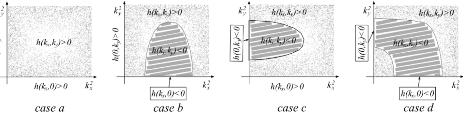
Summing up we have demonstrated that patterns can eventually develop only if the system can undergo a symmetry breaking instability of the Turing type, in its restricted configuration where the diffusion is solely allowed along one spatial direction, either x or y. The result is summarized in Figure 1, where different types of instabilities are schematically depicted.
Interestingly, the instability can set in also if the inhibitor diffuses slower that the activator along one selected direction, provided the opposite holds for the transport along the orthogonal direction. In this respect, accounting for anisotropic diffusion enables one to partially relax the stringent conditions that underly the formation of the Turing motifs. In the next section, we will built on this observation and provide a numerical demonstration of the investigated phenomenon.
6 k2 x k2 y h(k ,k )<0x y h(k ,0)<0x h(0 ,k ) > 0 y h(k ,k )>0x y k2 x k2 y h(k ,k )<0x y h(k ,0)<0x h(0 ,k ) < 0 y h(k ,k )>0x y k2 x k2 y h(k ,k )<0x y h(0 ,k ) < 0 y h(k ,0)>0x h(k ,k )>0x y k2 x k2 y
case b
h(0 ,k ) > 0 y h(k ,k )>0 x y h(k ,0)>0xcase a
case c
case d
FIG. 1: Possible types of instabilities. Case a: h(kx, ky) > 0 for all k2
x ≥0 and k
2
y ≥0. The system cannot turn unstable.
Case b: h restricted to the kxaxis takes negative values: a bounded contiguous domain in k2
x >0 and k
2
y>0 exist, for which
h(kx, ky) > 0. Case c: h restricted to the ky axis takes negative values. Again a portion of the reference plan, adjacent to
the domain of instability in kx= 0, can be found where h(kx, ky) > 0: Case d: the system is unstable along both kx= 0 and
ky= 0 directions. The instability also interests non trivial modes with both kx̸= 0 and ky̸== 0.
IV. NUMERICAL ANALYSIS
The aim of this section is to discuss a numerical implementation of the theory presented above. In particular, we will show that complex patterns can emerge for a system of two species in mutual interaction and undergoing anisotropic diffusion, also if the conventional Turing request of having inhibitors faster than activators is relaxed, along one of the two orthogonal directions of movements. To perform the analysis we operate in the framework of the so called Mimura-Murray model [8]. The quantities u and v can be associated to prey and predator densities, which interact via the non-linear functions:
f (u, v) =.(a + bu − u2)/c − v/ u and g(u, v) = (u − (1 + dv)) v ; (18)
the model possesses 6 equilibria, whose stability and positivity depend on the value of the chosen parameters. We here focus on the fixed point (ˆu, ˆv)
ˆ u = 1 +bd − 2d − c + √ ∆ 2d and ˆv = bd − 2d − c +√∆ 2d2 where ∆ = (bd − 2d − c) 2+ 4d2 (a + b − 1) , (19) and assume a = 35, b = 16, c = 9 and d = 0.4 which in turn implies (ˆu, ˆv) = (5, 10). Moreover, the Jacobian entries evaluated at the fixed point reads fu = 3.33, fv = −5, gu = 10 and gv = −4. Hence, det(J) > 0 and tr(J) < 0:
the fixed point is a stable equilibrium. We also remark that u acts as the activator and v stands for the inhibitor species, as fu > 0 and gv < 0. Under specific conditions, the fixed point can be destabilized by an external, non
homogeneous, perturbation, paving the way to the subsequent generation of Turing patterns, in the non linear regime of the evolution. In Fig. 2 we report a gallery of representative patterns that can be obtained under distinct conditions. To generate the asymptotic patterns displayed in panel (a) of Fig 2, parameters are set so that both relations (10) and (11) are satisfied, D(x)v > D(x)u rc and D
(y)
v > D(y)u rc, where rc ∼ 16. Inhibitor diffuses faster than activators
in both x and y directions, although with different diffusion constants. The dispersion relation (see Fig 2(b)) can be assimilated to that sketched in Fig. 1(d), and the corresponding patterns share marked similarities with those obtained in the conventional case of isotropic transport.
In panel (c) of Fig. 2, conditions (10) hold, while (11) do not, D(x)v > Du(x)rc while D(y)v < D(x)u rc, where rc ∼ 16.
The dispersion relation, Fig. 2(d), is also depicted and shown to resemble that displayed in Fig. 1(c). The patterns which follow this unusual choice of the diffusion constants, compare nicely with those emerging under the standard paradigm, this is because D(y)v /Du(x) is smaller but close to rc.
Finally, in panel (e,f) of Fig 2, the activator is assigned a diffusion coefficient D(y)u is larger than D(y)v , the homologous
constant associated to the inhibitor species, and still Dv(x) > D(x)u rc. The dispersion relation falls in the category
exemplified in Fig. 1(c), and the corresponding patterns are found to organize in regular stripes, which run almost parallel to the direction where the instability is present.
7 0 2 4 6 8 10 0 2 4 6 8 10 y x −8 −7 −6 −6 −5 −5 −5 −4 −4 −4 −4 −3 −3 −3 − 3 −2 −2 −2 −2 −1 −1 −1 − 1 −1 0 0 0 0 0 −4 − 4 −3 −2 −1 k y k x 0 5 10 15 20 0 5 10 15 20 −8 −7 −6 −5 −4 −3 −2 −1 0 (a) (b) 0 2 4 6 8 10 0 2 4 6 8 10 y x −8 −7 −6 −6 −5 −5 −5 −4 −4 −4 −4 −3 −3 −3 −3 −3 −2 −2 −2 − 2 −2 −1 −1 −1 − 1 −1 −4 − 4 0 0 0 0 0 −3 −2 −1 k y k x 0 5 10 15 20 0 5 10 15 20 −8 −7 −6 −5 −4 −3 −2 −1 0 (c) (d) 0 2 4 6 8 0 2 4 6 8 y x 3.5 4 4.5 5 5.5 6 −9 −8 −8 −7 −7 −7 −6 −6 −6 −6 −5 −5 −5 −5 −5 −5 −4 −4 −4 −4 −4 −4 −3 −3 −3 −3 −3 −2 −2 − 2 −2 −4 −4 −4 −1 −1 −1 −3 −3 −3 −2 −2 −1 −1 0 k y k x 0 5 10 15 20 0 5 10 15 20 −9 −8 −7 −6 −5 −4 −3 −2 −1 0 (e) (f)
FIG. 2: Asymptotic activator distribution: the concentration u(x, y, t) is displayed for sufficiently large t. Panel (a): Du(y)= 0.01,
Dv(y) = 0.16, D (x) u = 0.02, D (x) v = 0.32. Panel (b): D (y) u = 0.01, D (y) v = 0.155, D (x) u = 0.02, D (x) v = 0.32. Panel (c): Du(y)= 0.012, D (y) v = 0.01, D (x) u = 0.02, D (x)
v = 0.32. The other parameters are set to a = 35; b = 16; c = 9; d = 0.4. The filled
black squares identify the position of the maximum of the dispersion relation.
V. CONCLUSIONS
In this paper we elaborated on the impact of anisotropic diffusion for the emergence of Turing patterns in reaction– diffusion systems. We have in particular focused on systems of two interacting species confined in a rectangular, continuum domain, endowed with periodic boundary conditions. With reference to this paradigmatic case study, we have shown that a symmetry breaking instability of the Turing type can occur only if patterns do exist when diffusion is impeded along one of the two accessible directions. In other words, patterns which resemble those obtained in the conventional setting of isotropic diffusion emerge, also when the standard Turing condition is violated along one specific direction. Interestingly, the instability can also occur if the activator diffuses faster than the inhibitor, along
8
the direction of spatial relocation for which the usual Turing conditions are not met.
Acknowledgments
The work of T.C. presents research results of the Belgian Network DYSCO (Dynamical Systems, Control, and Optimization), funded by the Interuniversity Attraction Poles Programme, initiated by the Belgian State, Science Policy Office.
[1] Asllani M., Di Patti F., Fanelli D., Stochastic Turing patterns on a network Phys. Rev E, 86, 046105 (2012)
[2] Asllani M., Biancalani T., Fanelli D., McKane A.J., The linear noise approximation for reaction-diffusion systems on
networks EPJB, 86, 476 (2013)
[3] Belousov B. P. , Periodically acting reaction and its mechanism Collection of Abstracts on Radiation Medicine, 145, 147 (1957)
[4] Biancalani T., Di Patti F., Fanelli D., Stochastic Turing patterns in the Brusselator model Phys. Rev E, 81, 046215 (2010) [5] Cantini L., Cianci C., Fanelli D., Massi E., Barletti L., Asllani M, Stochastic amplification of spacial modes in a system
with one diffusing species J. Math. Biol, DOI 10.1007/s00285-013-0743-x (2013)
[6] R. deForest and A. Belmonte, Spatial pattern dynamics due to the fitness gradient flux in evolutionary games Phys. Rev. E., 87, 062138 (2013)
[7] Ermentrout B., Lewis M., Pattern formation in systems with one spacially distributed species Bull Math Biol 59(3), 533-549 (1997)
[8] Mimura, M. and Murray, J. D., Diffusive prey-predator model which exhibits patchiness J. Theor. Biol. 75, 249 (1978) [9] Murray J. D., Mathematical Biology II: Spatial Models and Biomedical Applications Springer–Verlag, (2003)
[10] M.A. Novak and R.M. May, Evolutionary games and spatial chaos Nature, 359, 827 (1992)
[11] M.A. Novak and S. Bonhoeffer and R.M. May, More spatial games Int. J. Bifurcation Chaos, 4, 33 (1993)
[12] Ord A., Hobbs B. E., Fracture pattern formation in frictional, cohesive, granular material Phil. Trans. R. Soc. A, 368, 95 (2010)
[13] R. A. Satnoianu and M. Menzinger and P.K. Maini, Multispecies reaction diffusion models and the Turing instability
revisited Math. Biol., 41, 493 (2000)
[14] Strogatz S., Non linear dynamics and chaos: with applications to Physics, Biology, Chemistry and Engineering Perseus Book Group (2001)
[15] A. M. Turing, The Chemical Basis of Morphogenesis Phils Trans R Soc London Ser B, 237, 37 (1952)
[16] L. Yang and M. Dolnik and A. M. Zhabotinsky and E. R. Epstein, Pattern formation arising from interaction between
Turing and waves instabilityJournal of chemical physics, 117, 7259 (2002)