Quantum Chemical Methods for Predicting and Interpreting Second-Order Nonlinear Optical Properties: from Small to Extended π-Conjugated Molecules

RESEARCH OUTPUTS / RÉSULTATS DE RECHERCHE

Author(s) - Auteur(s) :

Publication date - Date de publication :

Permanent link - Permalien :

Rights / License - Licence de droit d’auteur :

Bibliothèque Universitaire Moretus Plantin

Institutional Repository - Research Portal

Dépôt Institutionnel - Portail de la Recherche

researchportal.unamur.be

Quantum Chemical Methods for Predicting and Interpreting Second-Order Nonlinear Optical Properties

Champagne, Benoît; Beaujean, Pierre; De Wergifosse, Marc; Hidalgo Cardenuto, Marcelo; Liégeois, Vincent; Castet, Frédéric

Published in:

Frontiers in Quantum Chemistry

Publication date:

2018

Document Version

Publisher's PDF, also known as Version of record

Link to publication

Citation for pulished version (HARVARD):

Champagne, B, Beaujean, P, De Wergifosse, M, Hidalgo Cardenuto, M, Liégeois, V & Castet, F 2018, 'Quantum Chemical Methods for Predicting and Interpreting Second-Order Nonlinear Optical Properties: from Small to Extended -Conjugated Molecules', Frontiers in Quantum Chemistry, pp. 117-138.

General rights

Copyright and moral rights for the publications made accessible in the public portal are retained by the authors and/or other copyright owners and it is a condition of accessing publications that users recognise and abide by the legal requirements associated with these rights. • Users may download and print one copy of any publication from the public portal for the purpose of private study or research. • You may not further distribute the material or use it for any profit-making activity or commercial gain

• You may freely distribute the URL identifying the publication in the public portal ?

Take down policy

If you believe that this document breaches copyright please contact us providing details, and we will remove access to the work immediately and investigate your claim.

Quantum Chemical Methods

for Predicting and Interpreting

Second-Order Nonlinear Optical

Properties: From Small to Extended

π-Conjugated Molecules

Benoît Champagne, Pierre Beaujean, Marc de Wergifosse,

Marcelo Hidalgo Cardenuto, Vincent Liégeois and Frédéric Castet

Abstract This chapter addresses the methodological and computational aspects

related to the prediction of molecular second-order nonlinear optical properties, i.e., the first hyperpolarizability (β), by using quantum chemistry methods. Both small (reference) molecules and extended push-pull π-conjugated systems are considered, highlighting contrasted effects about (i) the choice of a reliable basis set together with the convergence of β values as a function of the basis set size, (ii) the amplitude of electron correlation contributions and its estimate using wave function and density functional theory methods, (iii) the description of solvent effects using implicit and explicit solvation models, (iv) frequency dispersion effects in off-resonance conditions, and (v) numerical accuracy issues. When possible, comparisons with experiment are made. All in all, these results demonstrate that the calculations of β remain a challenge and that many issues need to be carefully addressed, pointing out difficulties toward elaborating black-box and computa-tionally cheap protocols. Still, several strategies can be designed in order to achieve a targeted accuracy, either for reference molecules displaying small β responses or for molecules presenting large β values and a potential in optoelectronics and photonics.

B. Champagne (_✉) ⋅ P. Beaujean ⋅ M. de Wergifosse ⋅ M.H. Cardenuto ⋅ V. Liégeois Laboratoire de Chimie Théorique, Unité de Chimie-Physique Théorique et Structurale, Université de Namur, rue de Bruxelles 61, 5000 Namur, Belgium

e-mail: benoit.champagne@unamur.be M.H. Cardenuto

Instituto de Física, Universidade de São Paulo, 66318, 05314-970 São Paulo, SP, Brazil F. Castet

UMR 5255 CNRS, Institut des Sciences Moléculaires (ISM), Université de Bordeaux, Cours de la Libération, 351, 33405 Talence Cedex, France

© Springer Nature Singapore Pte Ltd. 2018

M.J. Wójcik et al. (eds.), Frontiers of Quantum Chemistry, https://doi.org/10.1007/978-981-10-5651-2_6

Keywords First hyperpolarizability

⋅

⋅

⋅

⋅

6.1 Introduction

The molecular properties known as the (electric dipole) polarizability (α), first (β) and second (γ) hyperpolarizabilities, are defined by a phenomenological equation describing the change in the electric dipole moment that results from the application of external electric fields:

Δμζ= ∑ x, y, z η αζηð −ωσ; ω1ÞFηð Þ +ω1 _{2! ∑}1 x, y, z η, χ β_{ζηχð −ω}σ; ω1, ω2ÞFηð ÞFω1 χð Þω2 + 1 3! ∑ x, y, z η, χ, ξ γ_ζηχξð−ωσ; ω1, ω2, ω3ÞFηð ÞFω1 χð ÞFω2 ξð Þ + . . .ω3 ð6:1Þ

where Fηð Þ is the amplitude of the field oscillating at pulsation ωω1 1and applied in

the η direction and ωσ= ∑iωi. For more than a century in the case of the

polar-izability and half of that period for the higher-order responses, these properties have been the topic of intense activities among theoretical chemists and physicists. On the one hand, efforts have been devoted to the very accurate evaluation of these properties for atoms (i.e., α and γ because β is zero by symmetry) and small molecules with the aim of providing reference values for experiments, which usually rely on relative rather than on absolute measurements [1, 2]. This has stimulated extensive methods developments to account for electron correlation effects, frequency dispersion, vibrational contributions, as well as solvent effects. Small systems are also ideal to assess the reliability of new quantum chemistry methods because of reduced needs in computational resources. On the other hand, owing to their potential for achieving large nonlinear optical (NLO) responses, organic and mixed organic–inorganic chromophores were also the object of a large number of theoretical investigations, which allowed establishing structure–property relationships [3, 4]. These theoretical guidelines allowed designing molecular systems for applications in photonics and sensing devices, as well as for bio-imaging [5, 6].

This chapter discusses the use of quantum chemistry methods to calculate and interpret the NLO responses from small molecules to extended push-pull π-conjugated systems. This topic being very broad, the focus is restrained to the first hyperpolarizability rather than to both the first and second hyperpolarizabilities, and to the electronic response, leaving the pure vibrational and zero-point vibra-tional average counterparts for another contribution. Then, such quantum chemistry applications are illustrated in domains recently tackled by the authors. In particular, the discussion focuses on quantities that can be extracted from experimental

measurements, namely the hyper-Rayleigh scattering (HRS) hyperpolarizability, βHRS, and the associated depolarization ratios (DR), or the electric field-induced

second harmonic generation (EFISHG) response, β//. The expressions of the HRS

responses involve ensemble averages over the molecular orientations:

β_{HRSð−2ω; ω, ωÞ =}q"ffiffiffiffiffiffiffiffiffiffiffiffiffiffiffiffiffiffiffiffiffiffiffiffiffiffiffiffiffiffiffiffiffiffiffiffi⟨β_ZZZ2 ⟩ + ⟨β2_ZXX⟩# ð6:2Þ

DR = ⟨β2ZZZ⟩

⟨β2ZXX⟩ ð6:3Þ

in which X and Z are axes of the laboratory frame. The expressions of ⟨β2ZZZ⟩ and

⟨β2_ZXX⟩ in terms of Cartesian molecular tensor components can be found in Ref. [7]. The EFISHG response corresponds to the projection of the vector part of β on the dipole moment vector:

β _{̸̸ð−2ω; ω, ωÞ =} 1 5 ∑_i μ_i jμ⃗j∑j ðβijj + β_jij+ β_{jjiÞ =} 3 5 ∑_i μ_iβ_i jμ⃗j ð6:4Þ

6.2 Small Molecules in Gas Phase

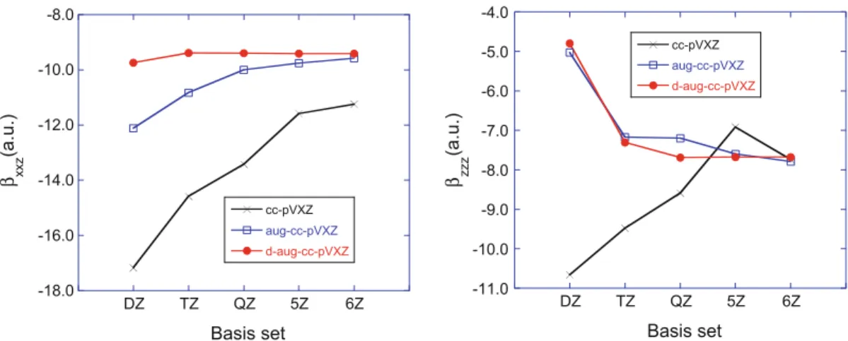
A first element for accurately predicting the responses of small molecules is the selection of a sufficiently flexible atomic basis set, generally containing many polarization and diffuse functions. Diffuse functions are needed because a sub-stantial part of the response originates from the outer and most diffuse part of the electron density. The need for polarization functions can easily be understood by noticing that the successive first-, second-, … order responses of a spherical (s) atomic orbital to an external field can be described by p-like, d-like, … func-tions. So, some authors have privileged adding selected diffuse and/or diffuse polarization functions to basis sets employed for geometry optimizations and thermodynamics [8–10]. Others have designed property-oriented basis sets [11,12] or have used basis sets constructed by adding even-tempered sets of diffuse func-tions to the correlation consistent basis sets of Dunning and co-workers [13], showing that with multiple-augmented sets the electrical properties of small molecules converge smoothly [14]. This is illustrated in Fig. 6.1for the main static β tensor components of the water molecule, calculated at the Hartree–Fock level. Alternatives to these atomic basis set approaches consist in employing a fully numerical approach [15, 16].

Then, electron correlation should be included at a sufficiently high level of approximation to achieve quantitative accuracy. Several levels of approximation and techniques are available. The easiest technique consists in calculating β from finite differentiation of the field-dependent energy of the molecule. This is the finite

field (FF) method [17] that simply requires adding the electric dipole interaction term, _{−μ⃗̂⋅E⃗, to the Hamiltonian. Still, the field amplitudes have to be carefully} chosen within a stability window to avoid two drawbacks: (i) Too small field amplitudes create a loss of accuracy on the energy values, which gets amplified during the successive numerical derivatives, and (ii) too large field amplitudes introduce high-order contaminations in the derivatives before leading to diver-gences as a result of the change of the ground state electron configuration [18]. Nevertheless, once the stability window is defined, the high-order contaminations can be systematically and recursively removed by using Richardson extrapolation or polynomial fitting. These aspects have been recently reviewed [19, 20]. The FF approach has been employed to calculate the static HRS response, βHRS, of five

reference molecules, CCl4, CHCl3, CH2Cl2, CCl3CN, and CH3CN [14]. Results

sketched in Fig. 6.2show that electron correlation effects might be quite different as a function of the chemical nature. Considering the CCSD(T) results as the refer-ence, general—but not systematic—trends are observed. First, the HF values generally underestimate the CCSD(T) results, up to 50% in the case of CH3CN. An

improvement is achieved by using the second-order Møller–Plesset (MP2) pertur-bation theory method so that the MP2 values underestimate or overestimate the CCSD(T) values by up to 20–25%. Finally, missing the perturbative triples, the βHRSresponses are underestimated by up to 15% for CCl4and CCl3CN, whereas the

difference with respect to CCSD(T) is much smaller for compounds with fewer chlorine atoms (less than 1% and 6% for CH3CN and CH2Cl2, respectively).

Alternatively, β can be calculated by employing response function approaches [21, 22], which are equivalent to evaluate analytically the responses of the dipole moment to external fields oscillating at finite frequencies. At the HF level, this approach gives rise to the time-dependent HF (TDHF) method [23]. Within the density functional theory (DFT) formalism, it gives the time-dependent DFT (TDDFT) scheme [24]. A hierarchy of coupled-cluster (CC) models has also been

-18.0 -16.0 -14.0 -12.0 -10.0 -8.0 DZ TZ QZ 5Z 6Z cc-pVXZ aug-cc-pVXZ d-aug-cc-pVXZ β xxz (a.u.) Basis set -11.0 -10.0 -9.0 -8.0 -7.0 -6.0 -5.0 -4.0 DZ TZ QZ 5Z 6Z cc-pVXZ aug-cc-pVXZ d-aug-cc-pVXZ β zzz (a.u.) Basis set

Fig. 6.1 Evolution of the amplitude of the two dominant components of the static β tensor of the

water molecule calculated at the coupled-perturbed HF level by using the cc-pVXZ, aug-cc-pVXZ, and d-aug-cc-pVXZ basis set suites

elaborated: CCS=CIS, CC2, CCSD, and CC3, which allows controlling the con-vergence of the responses as a function of the level of treatment of electron cor-relation [22]. Figure 6.2_{illustrates the convergence of the EFISHG response, β}//, of

water as a function of the basis set and of the level of electron correlation. Like in Fig. 6.1, the convergence with basis set size is smooth, though it is faster at the HF and CCS level than when using higher-order methods. Then, for a given basis set, the ordering of the β// amplitudes according to the method is:

HF < CCS < CC3≈CCSD < CC2 ð6:5Þ Again, the contribution from the triples, as estimated from the difference between the CCSD and CC3 results, is small. On the other hand, the CC2 method overestimates β// by as much as 50%, whereas the β// amplitude is strongly

underestimated at the HF (40%) and CCS (20%) levels of approximation. For the CC levels, the β// amplitude ordering follows the relative values of the lowest

excitation energies, dominating the β response [25] (in the case of the1A1state, the

vertical excitation energies calculated with the d-aug-cc-pVTZ basis set amount to 10.79 eV (HF), 10.81 eV (CCS), 9.82 eV (CC3), 9.81 eV (CCSD), and 9.59 eV (CC2)).

Still, frequency-dependent hyperpolarizabilities evaluated at high-order electron correlation levels are not always available, so that various approximate schemes have been proposed. They combine static correlated values with static and dynamic responses evaluated at lower levels of approximation. A multiplicative or per-centage approximation (MA) has been proposed by Sekino and Bartlett [26], and an additive approximation (AA) by Rice and Handy [27]:

5.0 10.0 15.0 20.0 25.0 HF _MP2 MP4(DQ) _MP4(SDQ) CCSD CCSD(T) CCl₄ CHCl₃ CH₂Cl₂ CCl₃CN CH₃CN β HRS (static) -30.0 -25.0 -20.0 -15.0 -10.0 -5.0 1 2 3 4 CCS HF CC2 CCSD CC3 d-aug-cc-pVXZ β // (1064 nm)

Fig. 6.2 Basis set and electron correlation effects on β (a.u.). Left static βHRS of five reference

molecules evaluated with the d-aug-cc-pVTZ basis set; right dynamic β//(−2ω;ω,ω)

MA_βCCSD HRS ðωÞ = βCCSDHRS ð0Þ × βHF ̸DFT_{HRS ðωÞ} βHF ̸DFT_{HRS ð0Þ} ð6:6Þ AA_βCCSD HRS ðωÞ = βCCSDHRS ð0Þ + βHF ̸DFTHRS ðωÞ −βHF ̸DFTHRS ð0Þ $ % ð6:7Þ Besides their widespread use, these approximations have been assessed in a limited number of studies [28and references therein]. In the case of CCl4, both MA

and AA based on HF frequency dispersions underestimate βHRS (λ = 632 nm) by

about 20%, whereas for CH2Cl2, the underestimation is smaller with MA (8%) than

AA (12%). More drastically, the effect of the frequency dispersion of CCl4 is

qualitatively wrong when adopting the HF method, since it suggests a decrease of βHRS with the photon energy (Fig. 6.3), whereas CCSD calculations predict an

increase of its amplitude. A much less frequently used alternative consists in describing frequency dispersion at the TDDFT level. So, LC-BLYP and B3LYP behave better than HF for the CCl4 molecule with an increase of βHRS with the

frequency, though slightly slower than with CCSD. Similarly, for CH2Cl2,

LC-BLYP (B3LYP) closely reproduces the CCSD frequency dispersion with small overestimations (underestimations). M06 (data not shown) and BLYP frequency dispersions are also close to the CCSD reference for CH2Cl2, whereas for CCl4,

M06 overestimates it substantially. These differences of frequency dispersion can be related to the relative values of the excitation energies (smaller with B3LYP than with CCSD), as well as of the transition dipoles, and excitation-induced dipole moment variations.

Comparisons of the CC3/d-aug-cc-pVQZ β//values of H2O (−19.28 and −21.77

a.u. at 1064 and 694.3 nm, respectively) with experimental values (−19.2 ± 0.9 [29] and −22/0 ± 0.9 a.u. [30]) substantiate the predictability of the method and confirm the small amplitude of the vibrational contributions (note that the pure vibrational and zero-point vibrational average contributions might also be

1.0 1.1 1.2 1.3 1.4 CCl₄-HF CCl₄-CCSD CH₂Cl₂-HF CH₂Cl₂-CCSD β HRS (ω )/ β HRS (0)

Photon energy (eV)

1.0 1.1 1.2 1.3 1.4 0.0 0.5 1.0 1.5 2.0 0.0 0.5 1.0 1.5 2.0 CCl4-B3LYP CCl4-LC-BLYP CCl4-CCSD CH2Cl2-B3LYP CH2Cl2-LC-BLYP CH2Cl2-CCSD β HRS (ω )/ β HRS (0)

Photon energy (eV)

Fig. 6.3 Frequency dispersion on βHRSdescribed at the TDHF (left) or TDDFT (right) levels of

non-negligible while canceling each other). In the case of CCl4, Shelton [31]

reported an experimental βHRS(at 1064 nm) value of 12.8 ± 1.1 a.u. in comparison

with a theoretical estimate of 14.3 a.u. The latter value was obtained by adding to the electronic dynamic CCSD value (14.9 a.u.) [28], the ZPVA (_{−1.1 a.u.), and} pure vibrational (0.5 a.u.) contributions of [32].

Though small systems such as H2O, CCl4, and CH2Cl2 allow using

computa-tionally demanding techniques and therefore tackling the convergence of the molecular properties as a function of electron correlation level, it is worth assessing the reliability of more approximate schemes in view of applying these to larger systems. In particular, there is an interest to assess the performance of density functional theory (DFT) with conventional as well as with most recent exchange-correlation functionals in comparison with the Hartree–Fock method and to MP2. Following Ref. [33], different levels of approximation have been assessed in comparison with FF CCSD(T) calculations (Fig. 6.4). Systematic trends are observed: (i) BLYP overestimates βHRS by as much as 100% for CCl4; (ii) this

overestimation decreases when adding 20% of HF exchange (B3LYP) but not for CH2Cl2and CCl4with M06 (28% HF exchange) so that with these three functionals

the accuracy is lower than with HF, which underestimates βHRS by 15–30%;

(iii) then, further increasing the percentage of HF exchange (BHandHLYP (50%) and M06-2X (56%)) leads to improvements; and (iv) finally, range-separated hybrids perform also better, but the improvement is not systematic (CAM-B3LYP reproduces closely the response of H2O, but the error on CCl4 is as large as 40%,

whereas with LC-BLYP, βHRSof H2O is underestimated by 25% and the responses

of the two other compounds are close to CCSD(T)). On the other hand, Karamanis et al. [34_{] have shown that for doped Si clusters, hybrid GGA with 20–25% HF}

exchange performs better than hybrid GGAs with larger percentage of HF exchange or than long-range corrected hybrids. So, without considering push-pull π-conjugated systems for which the XC requirements are also function of their

-50.0 0.0 50.0 100.0 150.0 CCSD QRF-CCSD HF _MP2 BLYP _B3LYP BHandHLYP CAM-B3LYP LC-BLYP M06 M06-2X H 2O CH 2Cl2 CCl 4 Error (%) on β HRS with respect to CCSD(T) Methods Fig. 6.4 Error (%) on the

static βHRSof H2O, CH2Cl2,

and CCl4 for different

exchange-correlation functionals and levels of approximation in comparison with CCSD(T). The

calculations were performed with the d-aug-cc-pVTZ basis set. MP2, CCSD, and CCSD (T) results were obtained from the FF calculations, the QRF-CCSD calculations using the response method, and the HF and DFT calculations with the coupled-perturbed analytical differentiation procedures

size and charge-transfer character [35_–39], the reliability of DFT depends strongly on the XC functional and there is no easy clue to select a priori an accurate XC functional. Still, the best functionals are global or range-separated hybrids and include substantial amounts of HF exchange.

When using DFT approaches, an additional parameter to control is the density of the integration grid. The Gaussian09 grids are called Fine, UltraFine, and SuperFine, and they differ by the number of radial shells (75, 99, and 150, respectively) and of angular points per shell (302, 590, and 974). In a recent investigation [33], it was found that for TDDFT calculations of small reference molecules, the βHRS differences could attain up to 1 a.u. (up to 5%) between the

UltraFine and SuperFine grids when employing meta-GGA XC functionals, whereas this difference is only of _{∼0.02 a.u. when using GGA or hybrid XC} functionals. In fact, the situation is even more complex when considering that β tensor components can be evaluated from the FF approach as the first-, second-, and third-order derivatives. Let us consider the βzxx component:

β_zxx= ₋ ∂3E ∂E_z∂E2_x & ' 0 = ∂2μz ∂E_x2 & ' 0 = ∂αzx ∂E_x & ' 0 ð6:8Þ

For variational wave functions, these three quantities are expected to be identical and also identical to the fully analytical TDDFT/CPKS value. We have performed such FF calculations for βzxxof H2O. A selection of Romberg’s tables is provided in

Table 6.1. In these calculations, the threshold on the energy has been lowered to 10−11_{a.u. As discussed in the previous works [19,20], each table presents the same}

structure. In particular, for n = 0, by going from k = 0 to k = 6, the β values vary randomly until a given k value where β starts increasing monotonically. At smaller k’s, these variations originate from the lack of precision on the field-dependent properties (α, μ, or E). At larger k’s, the monotonic behavior results from the higher-order contaminations, which can then be iteratively and systematically removed using Romberg’s quadrature. This allows locating stability domains for β and therefore converged β values. Considering β as the first-order derivative of α, a converged value of 3.37 a.u. is obtained using a Fine grid. An UltraFine grid (as well as a SuperFine grid, results not shown) gives a value of 3.36 a.u. Analyzing the variations of βzxxas a function of the order of Romberg’s iteration (n)

and of the field amplitude (k) tells that the numerical accuracy on βzxxis of the order

of 0.01 a.u., consistently with an accuracy of 10−4 _{a.u. on the field-dependent}

polarizabilities. This value of 10−4 _{is obtained by taking the product between the}

accuracy on βzxxand the field amplitude for k = 4, which corresponds to the smallest

field amplitude associated with the converged value. A similar accuracy is achieved by considering the second-order derivative of μ with non-negligible differences in the Romberg’s tables when going from the UltraFine to the SuperFine grid and large differences between the Fine and UltraFine grids. This highlights a reduction of accuracy on the dipole moment values. Moreover, these data are con-sistent with an accuracy of about 10−6_{a.u. on the field-dependent dipole moments.}

Table 6.1 Romberg’s table for the evaluation of βzxx of H2O as a function of the order of the

derivative and the quality of the integration grid. The LC-BLYP XC functional was employed together with the aug-cc-pVTZ basis set. n represents the number of Romberg’s iterations, where higher-order contaminations are removed. k determines the field amplitude, E = E0 2k with

E0= 0.0004 a.u. Best/converged values are indicated by an arrow

n = 0 n = 1 n = 2 n = 3 n = 4 n = 5 n = 6 First-order derivative of α, grid = Fine

k = 0 3.37314 3.37341 3.37376 3.37387 3.37390 3.37391 3.37391 k = 1 3.37234 3.36812 3.36688 3.36655 3.36647 3.36645 k = 2 3.38499 3.38674 3.38730 3.38744 3.38747 k = 3 3.37975 3.37835 3.37863 3.37871 k = 4 3.38393 3.37414 3.37394 → 3.37 k = 5 3.41329 3.37707 k = 6 3.52197

First-order derivative of α, grid = UltraFine

k = 0 3.36461 3.36776 3.36869 3.36893 3.36899 3.36901 3.36901 k = 1 3.35517 3.35382 3.35355 3.35348 3.35346 3.35346 k = 2 3.35922 3.35792 3.35777 3.35774 3.35773 k = 3 3.36313 3.36009 3.35993 3.35989 k = 4 3.37223 3.36257 3.36252 → 3.36 k = 5 3.40122 3.36331 k = 6 3.51496

Second-order derivative of μ, grid = Fine

k = 0 4.25000 4.47188 4.52941 4.54396 4.54761 4.54853 4.54875 k = 1 3.58437 3.60885 3.61255 3.61331 3.61349 3.61354 k = 2 3.51094 3.55339 3.56461 3.56745 3.56816 k = 3 3.38359 3.38504 3.38557 3.38570 k = 4 3.37925 3.37708 3.37771 → 3.38 k = 5 3.38577 3.36750 k = 6 11.49397

Second-order derivative of μ, grid = UltraFine

k = 0 3.58750 3.63437 3.64684 3.65002 3.65082 3.65102 3.65107 k = 1 3.44688 3.44740 3.44630 3.44595 3.44585 3.44583 k=2 3.44531 3.46387 3.46843 3.46956 3.46985 k=3 3.38965 3.39538 3.39714 3.39758 k=4 3.37246 3.36898 3.36928 → 3.37 k=5 3.38290 3.36445 k=6 3.43824 (continued)

Table 6.1 (continued)

n = 0 n = 1 n = 2 n = 3 n = 4 n = 5 n = 6 Second-order derivative of μ, grid = SuperFine

k = 0 3.62500 3.63854 3.63778 3.63731 3.63718 3.63714 3.63713 k=1 3.58437 3.65000 3.66720 3.67156 3.67265 3.67292 k=2 3.38750 3.39193 3.39301 3.39328 3.39334 k=3 3.37422 3.37567 3.37631 3.37647 k=4 3.36987 3.36603 3.36626 → 3.37 k=5 3.38141 3.36261 k=6 3.43781

Third-order derivative of E, grid = Fine

k = 0 3.34710 3.34181 3.34038 3.34001 3.33992 3.33990 3.33989 k = 1 3.36296 3.36329 3.36343 3.36347 3.36348 3.36348 k = 2 3.36197 3.36121 3.36120 3.36119 3.36119 k = 3 3.36424 3.36146 3.36147 3.36147 → 3.361 k = 4 3.37256 3.36142 3.36135 k = 5 3.40599 3.36251 k = 6 3.53643

Third-order derivative of E, grid = UltraFine

k = 0 3.35632 3.35569 3.35560 3.35559 3.35558 3.35558 3.35558 k = 1 3.35820 3.35693 3.35664 3.35657 3.35655 3.35655 k = 2 3.36201 3.36129 3.36128 3.36128 3.36128 k = 3 3.36417 3.36135 3.36135 3.36135 → 3.361 k = 4 3.37262 3.36146 3.36139 k = 5 3.40608 3.36259 k = 6 3.53655

Finally, the best accuracy is achieved by considering the third-order derivative of the energy, leading to a value of 3.361 a.u. (if not 3.3613 a.u.). Using an UltraFine grid provides slightly more accurate results than the Fine grid, whereas there is almost no difference with the SuperFine grid. Further calculations were per-formed with a (very tight) threshold of 10−13a.u. on the energy, which is not going to work for any compound and the whole set of field amplitudes, and they did not lead to improvements. So, to get highly accurate results, a Fine grid can be used but in combination with third-order energy derivatives, whereas the UltraFine grid is recommended together with first-(second-)order derivatives of α (μ) because the number of significant digits on the energy is larger than on μ and on the CPKS α.

6.3 Small Molecules in Solution

Implicit solvation models like the polarizable continuum model (PCM) [40] are usually employed to account for the effects of solvation on the first hyperpolariz-ability. These models describe the solvent as a structureless polarizable continuum

characterized by, among other parameters, its macroscopic dielectric permittivity, which depends on the frequency of the applied field. For CCl4, the dielectric constant

or relative permittivity amounts to 2.23 (ε0) and 2.13 (ε∞) in the zero (static) and

infinite frequency limit, respectively. On the other hand, for CH2Cl2, the difference is

much larger with ε0 = 8.93 and ε∞ = 2.03, owing to the orientation contribution

related to the dipolar character of dichloromethane. This impacts directly the β responses, which are enhanced by the self-consistent reaction field. So, at the HF/d-aug-cc-pVTZ level, the βHRS,LIQ/βHRS,GAS ratio of CCl4amounts to 1.43 and

1.39 for infinite and 1064 nm wavelengths, respectively, whereas for the dipolar CH2Cl2, it goes from 2.39 to 1.78 [14]. Then, accounting for electron correlation

effects is not straightforward if the calculations are performed with the FF method, i.e., at zero frequency. Indeed, for dipolar solvents, the static dielectric constant is larger than the dynamic ones, which will lead to overestimations of the solvent effects and of the β amplitudes. A practical issue would be to use an effective static dielectric constant that only accounts for polarization contributions, neglecting the orientational contributions of the solvent. Another approach consists in correcting these static responses by including frequency dispersion with Eqs. 6.6and 6.7:

MA_βCCSD, PCM HRS ðωÞ = βCCSD, PCMHRS ð0Þ × βHF ̸DFT, PCM_{HRS ðωÞ} βHF ̸DFT, PCM_{HRS ð0Þ} ð6:9Þ AA_βCCSD, PCM HRS ðωÞ = βCCSD, PCMHRS ð0Þ + βHF ̸DFT, PCMHRS ðωÞ −βHF ̸DFT, PCMHRS ð0Þ $ % ð6:10Þ In this case, all the properties (the high-level static response as well as the static and dynamic TDHF or TDDFT responses) are performed using implicit solvation models. Consequently, two static β calculations are performed and their overesti-mations cancel each other, though incompletely. On the other hand, combining frequency dispersion as obtained from the two-state approximation [41] with high-level static PCM results will not be appropriate, besides in cases where an effective static dielectric constant is used.

Table 6.2 _{presents HRS quantities calculated for five reference molecules at the}

CCSD(T) level in combination with the MA scheme: βHRS, the depolarization ratio

(DR), which is determined by the shape of the NLOphore, the dipolar (|βJ=1|) and

octupolar (|βJ=3|) components, and their ratio, the nonlinear anisotropy parameter,

ρ = |βJ=3|/|βJ=1|. They are compared to the experimental values [14]. For all

com-pounds, the octupolar character is overestimated although the experimental ordering of the DR (and ρ) is reproduced. Additional calculations not reported here show that this hierarchy of DR is already reproduced at the HF level, but the underestimation of the DR values is more severe than at the CCSD(T) level. Then, considering that the standard deviations on the experimental values is typically of 10%, most of the calculated βHRS values match the experimental ones, in particular for CHCl3 and

CCl3-CN, but also for CH2Cl2 and CH3-CN, with errors smaller than 25%. On the

other hand, for CCl4, the underestimation is substantial and attains 50%. A large

Table 6.2 Dynamic (λ = 1064 nm) βHRS ,DR, |βJ=1 |, |βJ=3 |, and ρ values (a.u.) as determined at the CCSD(T)/d-aug-cc-pVTZ level of approximation using the MA scheme (Eq. 6.6 ) and accounting for solvent ef fects with the PCM approach in its Integral Equation Formalism (IEF) in comparison with experiment [ 14 ]. Values in parentheses are the dif ferences (%) with respect to the experimental values (for βHRS ) or the experimental values (DR and ρ) CCl 4 CHCl 3 CH 2 Cl2 CCl 3 – CN CH 3 – CN βHRS 13.73 (− 53) 19.74 (+4) 23.14 (+16) 22.41 (− 10) 40.48 (23) DR 1.50 (1.50) 1.90 (2.61 ± 0.02) 3.36 (4.21 ± 0.03) 2.16 (2.98 ± 0.03) 6.80 (8.40 ± 0.15) |βJ=1 | 0.00 17.89 37.02 25.10 81.77 |βJ=3 | 44.49 57.82 49.24 61.66 40.07 ρ ∞ (∞ ) 3.22 (1.84 ± 0.02) 1.33 (1.01 ± 0.01) 2.46 (1.54 ± 0.02) 0.49 (0.23 ± 0.15)

combined with CCSD(T) static responses [14] and, when describing frequency dispersion at the CCSD level as discussed in Sect. 2, the error is reduced by a factor of 2 [28]. These successive studies demonstrate that there is an interest in per-forming high-level calculations with explicit solvent molecules as well as in reassessing the amplitude of the vibrational contributions, the pure vibrational contribution that is usually negligible for the second harmonic generation and the zero-point vibrational average. In particular, the non-polar but highly polarizable CCl4 molecule appears to be a challenging case.

Still, for CCl4, these comparisons between experiment and theory assumed that

each molecule behaves like an independent light scatterer, giving rise to the so-called incoherent HRS signal, which is purely octupolar. Nevertheless, Kaatz and Shelton [42] have shown that the experimental HRS signal contains both a coherent (βcoh) and an incoherent (βincoh) part, with βcoh/βincoh ∼2/3. This coherent

response originates from the interactions between the CCl4molecules and attributes

to liquid CCl4 both dipolar (|βJ=1|) and octupolar (|βJ=3|) HRS responses. The

description of the dual contribution to βHRSof liquid CCl4 has been challenged by

sequential QMMM calculations. The method consists first in performing Monte Carlo simulations to generate uncorrelated snapshots representing the liquid structure [43, 44_{] and then in calculating at the QM level the first}

hyperpolariz-ability for a selection of these snapshots [45]. In these QM calculations, the solvent (surrounding molecules) is described either exclusively by point charges or by considering explicitly a few neighboring CCl4 molecules, embedded in point

charges of the remaining solvent molecules. It has been observed that considering explicitly a few neighboring CCl4 molecules embedded in point charges enables

monitoring the emergence of the dipolar contribution to βHRS,LIQ, characterized by

an increase of DR and a decrease of ρ. So, combining the Hartree–Fock method and the aug-cc-pVQZ basis set for feasibility purpose, with two interacting CCl4

molecules, DR attains 2.34 ± 0.66 (ρ = 2.11) while when considering five inter-acting molecules DR = 2.78 ± 0.92 (ρ = 1.81) [46]. Figure 6.5 illustrates the convergence of βHRS as a function of the number of snapshots in the case of five

interacting molecules embedded in point charges. Note that the amplitude of βHRS

per CCl4 molecule is little impacted when accounting for these specific

inter-molecular interactions. These calculations have confirmed to a large extent the experimental data and have substantiated that the dipolar contribution originates from intermolecular interactions between the CCl4 molecules. Nevertheless, it

remains challenging to perform high-level ab initio calculations on such CCl4

clusters, which expectedly will modify the description of the intermolecular inter-actions and their impact on βHRS, because calculating the first hyperpolarizability of

6.4 Extended p-Conjugated Dyes

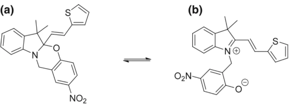
Basis set effects on the first hyperpolarizability of a π-conjugated dye were assessed in the case of an oxazine derivative (Scheme 6.1), which can switch between a closed and an open form upon triggering with light irradiation, as well as with pH and redox potential variations [47]. The calculations were performed at the TDHF level (λ = 1064 nm) on the closed form, which presents a rather small βHRS

response, and on the zwitterionic open form, whose βHRS is enhanced due to

push-pull electron delocalization effects. Solvent effects were accounted for by using the IEFPCM scheme [40]. Table 6.3_{reports the β}HRSvalues of the two forms,

their contrasts, βHRS(open)/βHRS(closed), and the corresponding depolarization

ratios. In the case of the closed form, starting from the 6-31G(d) basis set, adding

p polarization functions on the H atoms has a negligible impact on βHRS. On the

other hand, adding a set of sp diffuse functions leads to an increase of βHRSby 20%

while the addition of a second set of diffuse functions does not change significantly the βHRSvalues. Note that starting from the Dunning cc-pVDZ basis set, βHRSis 6%

smaller than with the 6-31G(d) basis while going to cc-pVTZ, cc-pVQZ, and cc-pV5Z leads to increases of 1%, 8%, and 13% with respect to 6-31G(d), respectively. However, these basis sets contain much more contracted GTOs than 6-31G(d). The 6-31G (and, to a lower extent, 6-311G) βHRSvalue is also larger than

the 6-31G(d) one, indicating that the inclusion of polarization and diffuse functions has counteracting effects. Finally, the values obtained with the aug-cc-pVDZ and aug-cc-pVTZ basis sets are in close agreement with those of the Pople basis set series, provided at least one set of diffuse functions is included.

The basis set effects are even smaller in the case of the oxazine open form. Indeed, going from 6-31G(d) to 6-31+G(d), βHRSincreases only by 12% while from

6-31G(d) to 6-31G βHRS increases by 3%. Then, the differences with respect to

6-31G(d) amounts to –2%, 1%, 4%, and 6% for cc-pVDZ, cc-pVTZ, cc-pVQZ, and

Fig. 6.5 Statistical

convergence of βHRSper CCl4

molecule calculated at the HF/aug-cc-pVQZ level as a function of the number of configurations (snapshots). Each calculation was

performed for a cluster of five molecules of CCl4solvated by

point charge embedding. The horizontal line gives the averaged value and the uncertainty corresponds to the statistical error

cc-pV5Z, respectively. Similarly, the aug-cc-pVDZ βHRSvalue is only 2% smaller

than the 6-31+G(d) value. Finally, the calculations performed with the aug-cc-pVTZ basis set, which, among those employed here, should be considered as the most flexible basis set for calculating the first hyperpolarizability, give βHRS

values slightly smaller than those obtained with the aug-cc-pVDZ (–1%), 6-31+G (d) (–4%), 6-31++G(d) (–4%), 6-311+G(d) (–4%), and 6-311++G(d) (–4%) basis sets.

(a) (b)

Scheme 6.1 Closed (left) and open (right) forms of an oxazine derivative. Switching from the

closed to open form can be triggered by light irradiation to form a zwitterion or by decreasing the pH to get the corresponding protonated cationic species [47]

Table 6.3 Effect of the basis set on the HRS first hyperpolarizability (βHRS) and its depolarization

ratio (in parentheses) of the closed (a) and open (b) forms of an oxazine derivative as well as on the βHRScontrast ratio, βHRS(open)/βHRS(closed). The calculations were performed at the TDHF

level with a wavelength of 1064 nm, while solvent (acetonitrile) effects were included using the IEFPCM scheme. The numbers in parentheses in the first column correspond to the number of contracted GTOs

βHRS(closed) βHRS(open) βHRS(open)/βHRS(closed)

6-31G (305) 841 (4.00) 3939 (5.94) 4.75 6-311G (445) 816 (3.89) 4019 (5.92) 4.92 6-31G(d) (479) 748 (4.11) 3824 (5.81) 5.12 6-31G(d,p) (539) 749 (4.11) 3830 (5.80) 5.11 6-311G(d) (590) 742 (4.00) 3903 (5.80) 5.26 6-31+G(d) (590) 895 (3.93) 4299 (5.92) 4.80 6-31++G(d) (615) 891 (3.90) 4290 (5.92) 4.81 6-311+G(d) (699) 914 (3.94) 4292 (5.95) 4.70 6-311+G(d,p) (759) 915 (3.93) 4298 (5.94) 4.70 6-311++G(d) (717) 910 (3.92) 4286 (5.95) 4.71 cc-pVDZ (510) 701 (3.96) 3748 (5.78) 5.34 cc-pVTZ (1154) 755 (3.94) 3880 (5.85) 5.14 cc-pVQZ (2199) 809 (3.97) 3984 (5.90) 4.92 cc-pV5Z (3743) 849 (4.00) 4057 (5.92) 4.77 aug-cc-pVDZ (848) 902 (4.00) 4194 (5.96) 4.65 aug-cc-pVTZ (1798) 897 (4.01) 4135 (5.95) 4.61

The combined effect of basis set extension on the first hyperpolarizability of the closed and open form results therefore in a slight decrease of the βHRS(open)/

βHRS(closed) contrast ratio, from 5.12 with 6-31G(d) to 4.71, 4.65, and 4.61 with

the 6-311++G(d), aug-cc-pVDZ, and aug-cc-pVTZ basis sets, respectively. Again, the 6-31G value is very close to the result obtained with the largest basis set. The effect of the basis set size on the depolarization ratio of both forms is also very weak, demonstrating that the dipolar versus octupolar contributions to βHRS are

already estimated within ±3% with the 6-31G(d) basis set. Still, increasing the basis set size decreases DR of the closed form (i.e., leads to a relative increase of the octupolar contribution), whereas for the open form, it leads to an increase of DR, or of the dipolar contribution to βHRS.

Consequently, in agreement with other studies [36], the requirements on the basis set are much less stringent for estimating βHRS and DR of a π-conjugated

push-pull molecule than for a small molecule.

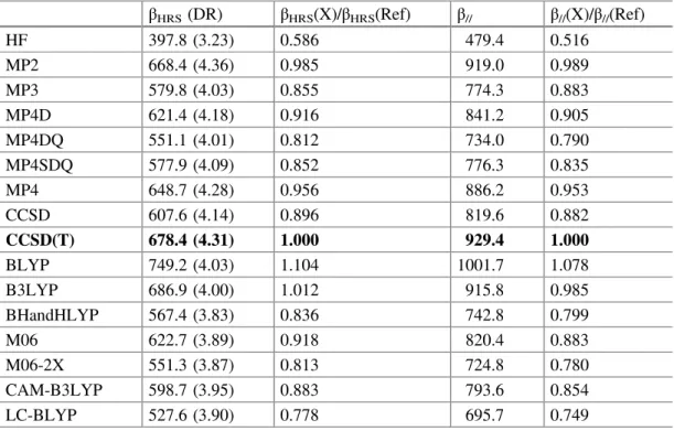
Electron correlation effects have then been analyzed in the case of p-nitroaniline, using the aug-cc-pVDZ basis set. Static β values have been obtained using the FF approach (Table 6.4_{). The same B3LYP/6-311G(d) geometry was used for all β}

calculations. Using the CCSD(T) results as references, the HF methodology strongly underestimates both βHRS and β// but most of the error is recovered by

including electron correlation at the second order (MP2). Then, higher-order cor-rections have detrimental or canceling contributions to β. Note that the inclusion of the triples (MP4 vs. MP4SDQ and CCSD vs. CCSD(T)) amounts to a correction of

Table 6.4 HRS and EFISHG first hyperpolarizabilities (βHRS and β//) (in a.u.) and HRS

depolarization ratios (DR) of p-nitroaniline as determined at different levels of approximation with the aug-cc-pVDZ basis set. All values have been obtained using the FF approach and are compared to the reference results obtained at the Ref = CCSD(T) level

βHRS(DR) βHRS(X)/βHRS(Ref) β// β//(X)/β//(Ref) HF 397.8 (3.23) 0.586 479.4 0.516 MP2 668.4 (4.36) 0.985 919.0 0.989 MP3 579.8 (4.03) 0.855 774.3 0.883 MP4D 621.4 (4.18) 0.916 841.2 0.905 MP4DQ 551.1 (4.01) 0.812 734.0 0.790 MP4SDQ 577.9 (4.09) 0.852 776.3 0.835 MP4 648.7 (4.28) 0.956 886.2 0.953 CCSD 607.6 (4.14) 0.896 819.6 0.882 CCSD(T) 678.4 (4.31) 1.000 929.4 1.000 BLYP 749.2 (4.03) 1.104 1001.7 1.078 B3LYP 686.9 (4.00) 1.012 915.8 0.985 BHandHLYP 567.4 (3.83) 0.836 742.8 0.799 M06 622.7 (3.89) 0.918 820.4 0.883 M06-2X 551.3 (3.87) 0.813 724.8 0.780 CAM-B3LYP 598.7 (3.95) 0.883 793.6 0.854 LC-BLYP 527.6 (3.90) 0.778 695.7 0.749

about 10%. The variations of DR are smaller but follow the same trends as those of βHRS, demonstrating that the inclusion of electron correlation mostly increases the

dipolar component of βHRS.

Using DFT and conventional XC functionals, the results get more contrasted. BLYP overestimates the β values (but not DR) by about 10%. Then, adding larger and larger amounts of HF exchange in the functional lead to a reduction of βHRSand

β// so that the agreement is excellent between B3LYP (20% HF exchange) and

CCSD(T), whereas the BHandHLYP (50% HF exchange) values are underesti-mated. Similar effects are observed between M06 (27% HF exchange) and M06-2X (54% HF exchange), where for the later the underestimations attain 20%, similar to what is found for BHandHLYP. The use of range-separated hybrids follows also the same trend with the smallest values obtained with the LC-BLYP functional (un-derestimations of 22 and 25%) and then CAM-B3LYP (un(un-derestimations of 12 and 15%). Indeed, at long range (r → ∞) LC-BLYP includes 100% of HF exchange, whereas CAM-B3LYP only 65%.

These results need however to be completed by those on other push-pull π-conjugated systems, with π-conjugated segments of different lengths and D/A groups of different strengths. In the case of α,ω-nitro, dimethylamino-polyenes containing 4 and 6 CH=CH units, the β(HF)/β(MP2) ratio amounts to 0.411 and 0.419, respectively [28]. Though these ratios have been obtained for the dominant longitudinal β tensor component with the 6-31+G(d) basis set, they can be compared with the β// ratio of 0.521 obtained here for p-nitroaniline. Similarly, the

corre-sponding values for the α,ω-nitro, dimethylamino-polyynes with 4 and 6 C ≡C units amount to 0.582 and 0.616, demonstrating that the β(HF)/β(MP2) ratio can vary by about 20% for π-conjugated segments commonly found in push-pull π-conjugated compounds. So, it is often recognized that the MP2/HF ratio for the static β values is close to 2 with a standard deviation of about 20%. Moreover, for those push-pull π-conjugated polyenes and polyynes containing 4 units, the β(MP2)/β(CCSD(T)) ratio amounts to 1.045 and 0.997 respectively, in comparison with a value of 0.989 for β// of p-nitroaniline, respectively. So, as substantiated by additional related

investigations [48, 49], for these compounds the MP2 approach is often a good compromise between accuracy and computational needs, but it requires using approximate schemes, like Eqs. 6.9–6.10, to describe frequency dispersion [20]. Still, benchmark results (CC3, CCSD, CCSD(T) together with a decent atomic basis set) on push-pull π-conjugated systems with 20–50 C atoms would be of high interest. Again, for systems different from (and usually larger than) p-nitroaniline, the selection of a reliable XC functional for evaluating β and its modifications upon chemical changes is a subtle issue, which was already addressed in depth in many studies [35–39, 48, 50]. For medium-size compounds, the range-separated LC-BLYP hybrid functional has been shown to be reliable when characterizing the changes of β upon enlarging the π-conjugated linker from 4 to 6 CH=CH (or C_{≡C) units or upon changing the polyyne linker into a polyene segment [}36]. On the other hand, the BLYP, B3LYP, and BHandHLYP functionals—as well as functionals with similar characteristics—generally perform quantitatively better, but the above chemical/size trends are poorly described. For instance, using the

6-31G(d) basis set, the β(B3LYP)/β(CCSD(T)) ratio amounts to 0.648 and 0.714 for the substituted polyenes with N = 4 and 6 (NMe2-(CH=CH)N-NO2) but to

0.999 and 1.372 for their polyyne analogs (NMe2-(C≡C)N-NO2), respectively [36].

Then, going toward even larger oligomers, the unphysical delocalization inherent to conventional (LDA, GGA, meta-GGA, and global hybrids) XC functionals gives rise to overestimations of the hyperpolarizabilities by more than one order of magnitude. This can be corrected by enforcing an asymptotically correct exchange-correlation potential, i.e., 100% of Hartree–Fock exchange. Still, as shown by early works [50], global hybrids with 100% HF exchange merely reproduce the β values calculated at the Hartree–Fock level. On the other hand, range-separated or long-range corrected (LC) hybrids, where the percentage of HF exchange varies with the inter-electronic distance, bring an improvement. This is evidenced by the β results of Kamiya et al. [48_{] on α,ω-nitro, amino-polyenes,}

where the LC-BOP results are larger than the HF ones, though smaller than the MP2 values. A further refinement of the XC functional consists in adjusting the range-separated parameter (µ) such that Koopmans’ theorem is obeyed as closely as possible [51]. It is found that the optimal µ values are smaller than those recom-mended as standard values (0.30, 0.33 or 0.47 bohr−1_{) and that they increase as a}

function of the size of the π-conjugated segment. So, in the case of (E)-N, N-dimethyl-4-(4-nitrostyryl)aniline derivatives containing from N = 1 to 4 CH=CH units between the phenyl rings, the LC-PBE and LC-PBE0 functionals with the standard µ = 0.30 value underestimate the MP2 β values for N = 3–4 by 18% and 27%, whereas using the optimal µ value, the corresponding functionals overestimate β by 15–24% and 12–21%, respectively [38]. For these systems, using the optimal µ value does not represent a clear improvement, whereas these optimally tuned range-separated hybrids perform clearly better than the conventional ones for N = 1–2. The complexity of selecting an appropriate XC functional has been further evidenced in a recent work due to Isborn and co-workers [39], recom-mending a larger fraction of exact exchange when computing β than for computing excitation energies. Thus, it is not clear whether exchange hybrid functionals could be further optimized to qualitatively and quantitatively reproduce MP2–or CCSD (T)–β values of increasingly large push-pull π-conjugated systems or, in other words, whether non-local exchange is sufficient in the absence of non-local cor-relation. Indeed, double hybrids, which include a given percentage of MP2 corre-lation, can provide for medium-size push-pull π-conjugated systems β values of at least similar quality as the global hybrids. Therefore, combining the same optimally tuned range-separated strategy for both HF exchange and MP2 correlation might lead to a functional for accurate prediction of β. Note however that the inclusion of MP2 correlation should be accompanied with an improvement over MP2 because the contrary would simply substantiate the use of MP2 to approximate CCSD(T). Finally, the selection of an appropriate XC functional can also be addressed in the case of NLO switches (Scheme 6.2), molecules characterized by their ability to alternate between two or more chemical forms displaying contrasts in one of their NLO properties (here, the second harmonic intensity) [52]. In this case, besides the absolute values, their contrast is also of interest. Scheme 6.2gives the structure of a

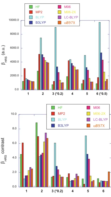
selection of NLO switches that have recently been studied [53–56] as well as the targeted contrast. The reported calculations were carried out using the 6-311+G(d) basis set. The same geometries were used for the whole set of β calculations. Some of these calculations were already reported in Refs. [52, 57]. These correspond to static βHRS values obtained in gas phase, except for compounds 6 where solvent

(ethanol) effects were accounted for using the IEFPCM scheme. The results are shown in Fig. 6.6_{. Again, there are large variations of β amplitudes among the}

different methods. Considering that the MP2 method provides reference values to

Scheme 6.2 Second-order NLO switches; 1–3 merocyanine–spiropyran with different

combina-tions of substituents [1: R1=NO2, R2=OMe, R3=Me, X=S, R4=R5=H; 2: R1=NO2, R2=NMe2,

R3=NH2, X=NMe, R4=H, R5=NO2; 3: R1=NO2, R2=NMe2, R3=NH2, X=NMe, R4=H,

R5=NO2] [53]; 4 neutral and protonated forms of a 4,5-dicyanoimidazole derivative [54]; 5

dihydroazulene (DHA)-vinylheptafulvene (VHF) [55]; 6 tautomeric equilibrium of the N-(2-hydroxynaphtylidene) aniline [56]

assess the XC functionals, the trend that the BLYP XC functional overestimates the static βHRS values of compounds 2–6 is confirmed (though for compound 4 the

agreement is better) and is related to the lack of HF exchange. Then, adding a small percentage of HF exchange (B3LYP and M06) improves the results for compounds

2 and 4, whereas large overestimations are still observed for 3, 5, and 6. Moving

from M06 to M06-2X leads to a further improvement for a third compound (3). Then, including long-range Hartree–Fock exchange (LC-BLYP and ωB97X) gives suitable results for compounds 2-6. All methods underestimate βHRSof compound 1

in its merocyanine form, and in all cases, the HF method underestimates βHRS, from

60% (1) to 37% (5).

Turning now to the contrasts, the BLYP, B3LYP, and M06 XC functionals can strongly underestimate or overestimate the βHRScontrasts. A clear improvement is Fig. 6.6 Comparisons

between HF, MP2, and DFT with different XC functionals to evaluate the static βHRSof

molecular switches.

(top) βHRSof chromophores

1–6 in one of their forms

(merocyanine form for 1–3; base form for 4, DHA form for 5, and enol form for 6) and (bottom) βHRScontrasts. The

“*0.2” and “*0.5” labels on the x-axis mean that the corresponding βHRSor βHRS

contrast values have been multiplied by the

corresponding factor, for a question of readability

achieved when using the M06-2X, LC-BLYP, and ωB97x functionals, at least for compounds 2–4, but a similar performance is achieved at the HF level. None of the methods is suitable to describe the βHRS contrasts of compounds 5 and 6,

high-lighting the difficulty in selecting a priori an XC functional to assess a broad variety of chromophores having second-order NLO responses.

Acknowledgements This work was supported by funds from the Belgian Government (IUAP N°

P7/5 “Functional Supramolecular Systems”) and the Francqui Foundation. It has also been done in the frame of the Centre of Excellence LAPHIA (Investments for the future: Programme IdEx Bordeaux–LAPHIA (ANR-10-IDEX-03-02)). V.L. thanks the Fund for Scientific Research (F.R. S.-FNRS) for his Research Associate position and M.H.C. the IUAP N° P7/5. The calculations were performed on the computing facilities of the Consortium des Équipements de Calcul Intensif (CÉCI, http://www.ceci-hpc.be), including those of the Technological Platform of High Perfor-mance Computing, for which we gratefully acknowledge the financial support of the FNRS-FNRC (Conventions 2.4.617.07.F and 2.5020.11) and of the University of Namur as well as on the “Mésocentre de Calcul Intensif Aquitain” (MCIA) of the University of Bordeaux, financed by the Conseil Régional d’Aquitaine and the French Ministry of Research and Technology.

References

1. D.P. Shelton, J.E. Rice, Chem. Rev. 94, 3–29 (1994)

2. T. Verbiest, K. Clays, V Rodriguez, Second-Order Nonlinear Optical Characterization Techniques: An Introduction (Taylor & Francis, 2009)

3. D.R. Kanis, M.A. Ratner, T.J. Marks, Chem. Rev. 94, 195–242 (1994)

4. J.L. Brédas, C. Adant, P. Tackx, A. Persoons, B.M. Pierce, Chem. Rev. 94, 243–278 (1994) 5. P.J. Campagnola, L.M. Loew, Nat. Biotechnol. 21, 1356–1360 (2003); Y.C. Liang, A.S.

Dvornikov, P.M. Rentzepis, Proc. Natl. Acad. Sci. USA 100, 8109–8112 (2003) 6. P.C. Ray, Chem. Rev. 110, 5332–5365 (2010)

7. R. Bersohn, Y.H. Pao, H.L. Frisch, J. Chem. Phys. 45, 3184–3198 (1966) 8. S.Y. Liu, C.E. Dykstra, J. Phys. Chem. 91, 1749–1754 (1987)

9. G.J.B. Hurst, M. Dupuis, E. Clementi, J. Chem. Phys. 89, 385–395 (1988)

10. S. Yamada, M. Nakano, I. Shigemoto, S. Kiribayashi, K. Yamaguchi, Chem. Phys. Lett. 267, 445–451 (1997)

11. T. Pluta, A.J. Sadlej, Chem. Phys. Lett. 297, 391 (1998); A. Baranowska, A.J. Sadlej, J. Comput. Chem. 31, 552–560 (2010); R. Zalesny, A. Baranowska-Laczkowska, M. Medved, J.M. Luis, J. Chem. Theor. Comput. 11,4119-4128 (2015)

12. G. Maroulis, J. Chem. Phys. 108, 5432–5448(1998); G. Maroulis, Theor. Chem. Acc.

129,437–445 (2011)

13. R.A. Kendall, T.H. Dunning Jr., R.J. Harrison, J. Chem. Phys. 96, 6796–6806(1992); D.E. Woon, T.H. Dunning Jr., J. Chem. Phys. 100, 2975–2988 (1994)

14. F. Castet, E. Bogdan, A. Plaquet, L. Ducasse, B. Champagne, V. Rodriguez, J. Chem. Phys.

136, 024506 (2012)

15. F.D. Vila, D.A. Strubbe, Y. Takimoto, X. Andrade, A. Rubio, S.G. Louie, J.J. Rehr, J. Chem. Phys. 133, 034111 (2010)

16. J.D. Talman, Phys. Rev. A 86, 022519 (2012)

17. H.D. Cohen, C.C.J. Roothaan, J. Chem. Phys. 43, S34 (1965) 18. D.M. Bishop, S.A. Solunac, Chem. Phys. Lett. 122, 567 (1985)

19. A.A.K. Mohammed, P.A. Limacher, B. Champagne, J. Comput. Chem. 34, 1497–1507 (2013)

20. M. de Wergifosse, V. Liégeois, B. Champagne, Int. J. Quantum Chem. 114, 900–910 (2014) 21. J. Linderberg, Y. Öhrn, Propagators in Quantum chemistry (Wiley-Interscience, Hoboken,

2004)

22. T. Helgaker, S. Coriani, P. Jørgensen, K. Kristensen, J. Olsen, K. Ruud, Chem. Rev. 112, 543 (2012)

23. S. Karna, M. Dupuis, J. Comput. Chem. 12, 487 (1991)

24. S.J.A. van Gisbergen, J.G. Snijders, E.J. Baerends, J. Chem. Phys. 109, 10657 (1998) 25. P. Beaujean, B. Champagne, J. Chem. Phys. 145, 044311 (2016)

26. H. Sekino, R.J. Bartlett, J. Chem. Phys. 94, 3665 (1991) 27. J.E. Rice, N.C. Handy, J. Chem. Phys. 94, 4959 (1991)

28. M. de Wergifosse, F. Castet, B. Champagne, J. Chem. Phys. 142, 194102 (2015) 29. P. Kaatz, E.A. Donley, D.P. Shelton, J. Chem. Phys. 10, 849 (1998)

30. J.F. Ward, C.K. Miller, Phys. Rev. A 19, 826 (1979) 31. D.P. Shelton, J. Chem. Phys. 137, 044312 (2012)

32. D.M. Bishop, F.L. Gu, S.M. Cybulski, J. Chem. Phys. 109, 8407 (1998) 33. F. Castet, B. Champagne, J. Chem. Theor. Comput. 8, 2044 (2012)

34. P. Karamanis, R. Marchal, P. Carbonnière, C. Pouchan, J. Chem. Phys. 135, 044511 (2012) 35. K.Y. Suponitsky, S. Tafur, A.E. Masunov, J. Chem. Phys. 129, 044109 (2008)

36. M. de Wergifosse, B. Champagne, J. Chem. Phys. 134, 074113 (2011) 37. S.I. Lu, C.C. Chiu, Y.F. Wang, J. Chem. Phys. 135, 134104 (2011) 38. H. Sun, J. Autschbach, ChemPhysChem 14, 2450–2461 (2013)

39. K. Garrett, X.A. Sosa Vazquez, S.B. Egri, J. Wilmer, L.E. Johnson, B.H. Robinson, C.M. Isborn, J. Chem. Theory Comput. 10, 3821–3831 (2014)

40. J. Tomasi, B. Mennucci, R. Cammi, Chem. Rev. 105, 2999–3094 (2005) 41. J.L. Oudar, D.S. Chemla, J. Chem. Phys. 66, 2664–2668 (1977)

42. P. Kaatz, D.P. Shelton, Mol. Phys. 88, 683–691 (1996)

43. K. Coutinho, S. Canuto, Adv. Quantum Chem. 28, 89–105 (1997)

44. K. Coutinho, R. Rivelino, H.C. Georg, S. Canuto, in Solvation Effects in Molecules and Biomolecules: Computational Methods and Applications (Springer, 2008), pp. 159–189 45. M. Hidalgo Cardenuto, B. Champagne, Phys. Chem. Chem. Phys. 17, 23634–23642 (2015) 46. M. Hidalgo Cardenuto, F. Castet, B. Champagne, RSC Adv. 6, 99558–99563 (2016) 47. E. Deniz, J. Cusido, S. Swaminathan, M. Battal, S. Impellizzeri, S. Sortino, F.M. Raymo,

J. Photochem. Photobiol., A 229, 20–28 (2012)

48. M. Kamiya, H. Sekino, T. Tsuneda, K. Hirao, J. Chem. Phys. 122, 234111 (2005); F. Bulat, A. Toro-Labbé, B. Champagne, B. Kirtman, W. Yang, J. Chem. Phys. 123, 014319 (2005) 49. B. Champagne, K. Kirtman, J. Chem. Phys. 125, 024101 (2006)

50. B. Champagne, E.A. Perpète, D. Jacquemin, S.J.A. van Gisbergen, E.J. Baerends, C. Soubra-Ghaoui, K.A. Robins, B. Kirtman, J. Phys. Chem. A 104, 4755–4763 (2000) 51. L. Kronik, T. Stein, S. Refaely-Abramson, R. Baer, J. Chem. Theory Comput. 8, 1515–1531

(2012)

52. B.J. Coe, Chem. Eur. J. 5, 2464–2471 (1999); J.A. Delaire, K. Nakatani K, Chem. Rev. 100, 1817–1845 (2000); I. Asselberghs, K. Clays, A. Persoons, M.D. Ward, J. McCleverty, J. Mater. Chem. 14, 2831–2839 (2004); F. Castet, V. Rodriguez, J.L. Pozzo, L. Ducasse, A. Plaquet, B. Champagne, Acc. Chem. Res. 46: 2656–2665 (2013)

53. A. Plaquet, M. Guillaume, B. Champagne, F. Castet, L. Ducasse, J.L. Pozzo, V. Rodriguez, Phys. Chem. Chem. Phys. 10, 3223–3232 (2008)

54. A. Plaquet, B. Champagne, J. Kulhanek, F. Bures, E. Bogdan, F. Castet, L. Ducasse, V. Rodriguez, ChemPhysChem 12, 3245–3252 (2011)

55. A. Plaquet, B. Champagne, F. Castet, L. Ducasse, E. Bogdan, V. Rodriguez, J.L. Pozzo, New J. Chem. 33, 1349–1356 (2009)

56. E. Bogdan, A. Plaquet, L. Antonov, V. Rodriguez, L. Ducasse, B. Champagne, F. Castet, J. Phys. Chem. C 114, 12760–12768 (2010)

57. A. Plaquet, B. Champagne, L. Ducasse, E. Bogdan, F. Castet, AIP Conf. Proc. 1642, 481–487 (2015)