HAL Id: tel-01870476
https://tel.archives-ouvertes.fr/tel-01870476
Submitted on 7 Sep 2018HAL is a multi-disciplinary open access
archive for the deposit and dissemination of sci-entific research documents, whether they are pub-lished or not. The documents may come from teaching and research institutions in France or abroad, or from public or private research centers.
L’archive ouverte pluridisciplinaire HAL, est destinée au dépôt et à la diffusion de documents scientifiques de niveau recherche, publiés ou non, émanant des établissements d’enseignement et de recherche français ou étrangers, des laboratoires publics ou privés.
To cite this version:
Lucas Pastor. Coloring, stable set and structure of graphs. Discrete Mathematics [cs.DM]. Université Grenoble Alpes, 2017. English. �NNT : 2017GREAM071�. �tel-01870476�
Présentée par
Lucas PASTOR
Thèse dirigée par Frédéric MAFFRAY, CNRS, et codirigée par Sylvain GRAVIER , CNRS
préparée au sein du Laboratoire des Sciences pour la
Conception, l'Optimisation et la Production de Grenoble
dans l'École Doctorale Mathématiques, Sciences et Technologies de l'Information, Informatique
Coloration, ensemble indépendant et
structure de graphe
Coloring, stable set and structure of graphs
Thèse soutenue publiquement le 23 novembre 2017, devant le jury composé de :
Monsieur FREDERIC HAVET
DIRECTEUR DE RECHERCHE, CNRS DELEGATION COTE D'AZUR, Rapporteur
Monsieur DIETER RAUTENBACH
PROFESSEUR, UNIVERSITE D'ULM - ALLEMAGNE, Rapporteur Monsieur LAURENT BEAUDOU
MAITRE DE CONFERENCES, UNIVERSITE CLERMONT AUVERGNE, Examinateur
Monsieur MICKAEL MONTASSIER
PROFESSEUR, UNIVERSITE DE MONTPELLIER, Examinateur Madame ALINE PARREAU
CHARGEE DE RECHERCHE,
CNRS DELEGATION RHONE AUVERGNE, Examinatrice Monsieur NICOLAS TROTIGNON
DIRECTEUR DE RECHERCHE, CNRS DELEGATION RHONE AUVERGNE, Président
Monsieur SYLVAIN GRAVIER
DIRECTEUR DE RECHERCHE, CNRS DELEGATION ALPES, Co-directeur de thèse
Monsieur FREDERIC MAFFRAY
DIRECTEUR DE RECHERCHE, CNRS DELEGATION ALPES, Directeur de thèse
Remerciements 7
1 Introduction (French) 13
1.1 Contenu du manuscrit . . . 18
2 Introduction 21 2.1 Context . . . 21
2.2 Outline of the manuscript . . . 26
2.3 Definitions . . . 26
2.4 Preliminaries . . . 27
3 Graph Coloring 33 3.1 Context and motivations . . . 33
3.1.1 Perfect graphs . . . 37
3.1.2 P`-free graphs . . . 41
3.2 Structure of (P6, bull)-free graphs . . . 44
3.2.1 General structure . . . 45
3.2.2 Brooms and magnets . . . 47
3.2.3 When there is no gem . . . 54
3.2.4 When there is a gem . . . 56
3.3 Coloring (P6, bull)-free graphs . . . 60
4 List Coloring 67 4.1 Context and motivations . . . 67
4.2 Structure of claw-free perfect graphs . . . 71
4.3 List coloring claw-free perfect graphs . . . 75
4.3.1 Peculiar Graphs . . . 76
4.3.2 Cobipartite graphs . . . 78
4.3.3 Elementary graphs . . . 86
4.3.4 Claw-free perfect graphs . . . 89
5.4 MWSS in (P7, bull)-free graphs . . . 112
6 Normal Graphs 121 6.1 Context and motivations . . . 121
6.2 The Probabilistic Method . . . 125
6.3 The random graph . . . 129
6.3.1 Properties . . . 129 6.3.2 The proof . . . 130 6.4 Proof of Lemma 6.16 . . . 134 Conclusion 139 Index of definitions 143 Index of symbols 145 Summary 155
1.1 An example of a map model. . . 15
1.2 Example of an optimal coloring. . . 16
1.3 Example of an optimal set S. Picked vertices are circled in purple. . . . 16
2.1 An example of a map model. . . 23
2.2 Example of an optimal coloring. . . 23
2.3 Example of an optimal set S. Picked vertices are circled in purple. . . . 24
2.4 Homogeneous set S, with A complete to S and B anticomplete to S. . . 28
2.5 A graph G and its modular decomposition tree T(G). . . 30
2.6 Creating a triangle in 8 operations. . . 31
3.1 A four coloring of the world map . . . 34
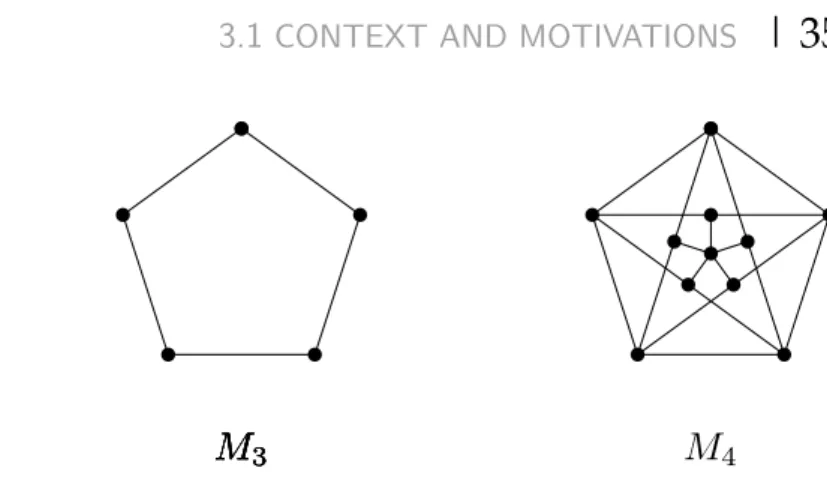
3.2 The first three Mycielski graphs. . . 35
3.3 Edge coloring example. . . 36
3.4 A graph G and its line-graph,L(G). . . 37
3.5 From left to right: C5, C7, C7. . . 38
3.6 The claw graph. . . 39
3.7 The diamond. . . 40
3.8 The bull. . . 41
3.9 The P6graph. . . 42
3.10 The graph Z2and the kite. . . 44
3.11 The double-wheel graph. . . 45
3.12 The broom. . . 47
3.13 Magnets . . . 51
3.14 The gem graph. . . 52
3.15 The partition of V(G) as in Theorem 3.30. A line between two sets represents partial or complete adjacency. No line means that the two sets are anticomplete to each other. . . 57
4.1 K2,4is not 2-choosable. . . 68
4.2 A partial latin square and its solution. . . 69
tation. . . 74
4.7 The graphs H4, H5and H6. . . 79
5.1 The graph S1,2,3. . . 96
5.2 The non-neighborhood K of the vertex v. . . 99
5.3 The 5-wheel graph. . . 99
5.4 From left to right: Umbrella, parasol, G1, G2. . . 100
5.5 The structure of a component in the non-neighborhood of v. . . 105
5.6 The graph G7. . . 107
6.1 The co-normal product of a graph G1with another graph G2. . . 122
6.2 A normal covering of K3. The clique is in orange (the whole graph) and the three stables are numbered from 1 to 3. . . 122
Tout d’abord, merci aux membres de mon jury d’avoir accepté de participer à la relecture et à la soutenance. Merci à mes rapporteurs Frédéric Havet et Dieter Rautenbach d’avoir relu ma thèse avec attention. Merci à Laurent Beaudou, Mickael Montassier, Aline Parreau et Nicolas Trotignon d’avoir apporté leur expertise le jour de ma soutenance. De nombreuses discussions enrichissantes ont pu émerger de mes travaux grâce à vous tous·tes.
C’est en cours de théorie des graphes en M2, sagement assis, que je me suis dit que ce serait intéressant de faire mon stage de fin d’études dans ce domaine. Sylvain, merci de m’avoir fait faire mes premiers pas en théorie des graphes, de m’avoir fait découvrir le monde de la coloration, de la coloration par liste et des graphes (parfaits) sans griffe. Grâce à toi, je me suis lancé dans ces recherches et encore aujourd’hui je m’y plaît énormément! J’ai également découvert Maths à Modeler grâce à toi. Je me suis familiarisé avec un autre aspect de la science extrêmement important à mon sens, à savoir faire découvrir, aux petits comme aux grands, la recherche scientifique. Enfin, je te remercie tout particulièrement d’avoir accepté de co-encadrer mon doctorat, sans toi je n’aurais pas pu faire cette thèse dans laquelle je me suis épanoui pendant ces trois années.
Frédéric, je ne sais même pas par où commencer pour te remercier tant tu as été important pour moi pendant mon doctorat. Dès notre première rencontre, et malgré mon inexpérience à l’époque, tu t’es montré bienveillant et pédagogue. Je me suis très vite rendu compte que tu connaissais un nombre incalculable de choses et, à chaque fois, tu as pris le temps de m’expliquer chacune d’entre elles. Je peux affirmer que pendant ces trois années de thèse, j’ai appris chaque jour quelque chose de nouveau, et tu as été, de loin, le plus grand contributeur à mon apprentissage. Ta porte était toujours ouverte (même quand je venais poser une question toutes les cinq minutes au commencement de ma thèse) et tu as été d’un soutien formidable et infaillible. J’ai également compris, grâce à toi, ce que voulait dire la célèbre expression “bien rédiger” (secrètement, je ressors encore de en temps en temps des passages de certains
de nos premiers articles pour m’en inspirer quand je rédige). Impossible de ne pas mentionner ta culture musicale digne d’une base de données. Je pense que tu vas plus vite qu’une requête SQL pour trouver le nom de l’artiste, la date, et le titre d’un morceau. C’est grâce à toi si je suis là aujourd’hui, si je me suis épanoui pendant ces trois années et si je continue à le faire encore aujourd’hui dans ma profession. Merci infiniment Frédéric.
Mes tous premiers petits pas en recherche, je les ai fait avec Francis Lazarus. Même si, à cette époque, j’étais bien loin de comprendre où je mettais les pieds, tu as pris le temps de me faire découvrir une partie de ce monde, et même de m’expliquer la Conjecture de Poincaré. Merci Francis de m’avoir ouvert cette porte et je ne te cache pas que j’ai l’espoir de pouvoir contribuer un jour à ton domaine!
Dear Ararat, I am switching especially to English for you, even though everybody knows that you are perfectly fluent in French now. Ararat, it is hard to express how sincere is my gratitude to you. You have taught me so many things and always have been so nice to me. We first met when I was just a PhD child and yet you decided to make me learn and take me on a scientific adventure. You have a kindness aura AND a fun aura that makes me feel good whenever I am around you. Thank you for everything Ararat.
C’est en L2 et L3 à Montpellier que je me suis dit pour la première fois: “mais, la théorie des graphes, c’est vraiment intéressant!”. C’était pendant un de tes cours, Stéphan, que j’ai accroché avec les graphes, la combinatoire, les maths discrètes. En commençant ma thèse, j’étais loin de m’imaginer que j’allais travailler avec toi. Tes cours et exposés m’ont toujours passionné et faire des maths à tes côtés a été sincère-ment inspirant. Je tiens à soulever ta gentillesse, notamsincère-ment lorsque tu expliques calmement, humblement et pédagogiquement que cette idée-là, tu y as aussi déjà pensé depuis deux heures, que tu as déjà fait le raisonnement complet et que tu es déjà en train de voir ce qu’il se passe au-delà de ce qu’on peut imaginer. Tu as pour moi un certain côté magique et je te remercie d’avoir pris le temps de partager, en toute humilité, une partie de tes connaissances avec moi ET de m’avoir fait découvrir les phrases du genre: “mais kiki là, il a forcément beaucoup de voisins dans B”.
Marthe, je me souviens de nos premiers échanges comme si c’était hier. Je te racon-tais que je travaillais sur de la coloration par liste, et j’ai pris le temps de t’expliquer maladroitement tout un tas de choses que tu connaissais déjà depuis longtemps. Et toi, tu étais là, à m’écouter patiemment, à attendre la fin de mon speech pour enfin prendre la parole et ajouter quelques théorèmes et problèmes ouverts à ce qui avait déjà été dit. Je ne savais pas à qui je parlais à l’époque, et justement tu es comme ça, humble. Impossible de ne pas remercier Nicolas Bonichon dans ce paragraphe, qui nous a calmement montré que savoir compter jusqu’à quatre peut se révéler intéres-sant. Ta puissance mathématique n’a d’égale que ta vitesse d’élocution, mais c’est vrai aussi pour ta gentillesse. Merci à toi Marthe pour tous ces moments à rire à ne plus pouvoir s’arrêter, ces moments de maths, et de m’avoir soutenu depuis notre première rencontre.
Je remercie également Pierre Aboulker, Julien Bensmail, Henning Bruhn-Fujimoto, Vincent Despré, Laura Gellert, Ross Kang, Arnaud de Mesmay, Jean-Florent
Ray-de m’apprendre à m’amuser en faisant Ray-des mathématiques, et Ray-de m’avoir toujours poussé à continuer.
Gaël, peut-être ne te souviens-tu pas des quelques discussions algébriques que nous avons eues il y a bien longtemps, ou encore du premier cours où tu m’as montré qu’on pouvait définir de nouvelles opérations différentes des usuelles. Sache que moi, en tout cas, je me souviens encore précisément que ces opérations avaient la forme de triangle, de carré et de rond. Merci à toi de m’avoir montré l’étendu inimaginable de ce monde.
Merci monsieur Toffoli pour avoir fait des cours de maths des moments où l’on s’amuse à chercher. Une citation inscrite sur un coin du tableau m’est restée: “Ils ne savaient pas que c’était impossible, alors ils l’ont fait”.
Je ne peux oublier le commencement de cette aventure qui remonte à l’année de mon Master 2 ROCO. Année pendant laquelle certes on ne comprenait pas toujours tout, mais pendant laquelle on a bien rigolé! Florence, Hugo, ce M2 était génial grâce à vous et vous avez été présents tout au long de ma thèse. Hugo, merci à toi pour tous ces bons moments et d’avoir été mon binôme dans cette dernière année d’études. Florence, ta porte était toujours ouverte quand j’errais dans les couloirs du 3H (c’est à dire tous les jours pendant trois ans) et il y avait toujours une place sur ton tableau pour que je puisse y dessiner un nouveau chef d’oeuvre chaque jour. Merci à toi d’avoir toujours été là, pour les nombreuses discussions sur la vie en général, et pour ton soutien infaillible.
Chaque jour de ma thèse, j’étais content de me lever et impatient d’arriver au laboratoire. Bien évidemment, ce genre de motivation n’est possible qu’avec une ambiance particulièrement bonne, sans aucun doute, présente à G-SCOP. Merci à l’équipe administrative, notamment Marie-Jo, toujours là pour aider! Ainsi qu’au service informatique, notamment Kevin et Olivier, qui m’ont aiguillé plus d’une fois. Merci à Alantha, Andrey, András, Andrea, Benjamin, Gautier, Hadrien, Matej, Myr-iam, Nadia, Olivier, Pierre Lemaire, et Zoltan auprès de qui j’ai eu l’occasion d’apprendre et/ou de recevoir du soutien et des encouragements tout au long de ma thèse. Louis, merci à toi pour les nombreuses discussions sur l’avenir que nous avons eues et sur les innombrables coups de main en tout genre que tu m’as rendus. Désolé encore pour le livre . . . Je tiens à soulever que j’ai été marqué par tes débuts de phrase “bon, j’y con-nais pas grand chose, mais”, suivi de pleins de concon-naissances précises qui prendraient trois surveys du domaine, et ça pour un nombre conséquent de notions! Depuis ce jour où j’ai été ton élève en M2, tu m’as beaucoup appris. Je te remercie pour tout ce que tu m’as apporté, parfois même sans le savoir.
Rémi, je dois dire que tu es bien le doctorant d’un de tes multiples papas de thèse (celui dont le livre nous sert de parapluie). Tu as redéfini ce que voulait dire pour moi “être bon en maths”. Tes connaissances générales en mathématiques m’ont toujours
impressionné (pas moyen que tu oublies un théorème, une preuve, ou une notion de mathématiques que tu as vue une fois dans ta vie). Mais surtout, tu as toujours partagé ces connaissances avec moi et tu m’as même poussé à me les approprier moi-même, à apprendre ou réapprendre des choses chaque jour avec un regard plus fin et plus précis. C’était un vrai plaisir d’être ton co-bureau durant ces trois années. Encore aujourd’hui il m’arrive de me dire: “Mince, si j’avais Rémi sous la main, cette preuve serait déjà terminée depuis longtemps . . . ”
Yohann, comment ne pas te citer dans mes remerciements de thèse. Merci à toi pour ces nombreuses discussions pleines de sagesse et de bienveillance. J’ai appris plus que des mathématiques à tes côtés et j’espère que nos chemins se recroiseront.
Quentin, merci à toi pour ces nombreuses discussions mathématiques passion-nantes, pour les petits problèmes (non triviaux!) que tu proposais parfois et pour l’effort de vulgarisation des règles de Magic dont tu faisais preuve à mon égard.
Nicolas Bousquet (je suis contraint de mettre ton nom de famille car il y a beau-coup de Nicolas dans notre monde). Merci à toi pour tout le soutien que tu m’as apporté, les relectures, et j’en passe. Sans oublier les encouragements. J’ai envie de dire, on peut avoir grandi à Mauguio et être quand même quelqu’un de très fort et très bien!
Aurélie, merci pour le nombre infini de coups de main par-ci, de coups de pouce par là, de discussions en tout genre, et surtout de grandes séances de rigolades qui font relativiser tout le reste. Ton talent, ta bonne humeur et la classe avec laquelle tu bois un Spritz sont une réelle inspiration.
Ces années à G-SCOP auraient été bien différentes sans la redoutable équipe de joyeux lurons qui suit, toujours prêts à faire une partie de coinche à midi et à se dé-tendre le soir venu. Alex, Aurélie, Clément, Élodie, Franck, Gricha, Laura, Lisa, Lu-cie, Matthieu, Nicolas Béraud, Nicolas Bousquet, Tom. Merci à vous tous pour ces moments passés ensemble, ces discussions tristes ou joyeuses, les (nombreuses) rigo-lades et les soirées qui, à elles seules, regroupaient tout ça. Un grand merci aussi à vous pour m’avoir soutenu à chaque instant, notamment en contribuant de manière conséquente à améliorer mes slides de soutenance. Vous êtes géniaux et je vous re-mercie pour tous ces moments inoubliables.
Sans le soutien inconditionnel de ma famille, je ne serais pas là où je suis au-jourd’hui. Merci à mon père et à ma mère qui ont toujours cru en moi. Merci à Marina pour sa bienveillance permanente qu’elle a depuis toujours. Merci à ma grand-mère qui en plus d’être la plus douée en informatique de la famille (et de loin. Mame, il y a encore de la place pour des nouvelles doctorantes en informatique si un jour tu en as l’envie) était celle à qui incombait la lourde tâche de me faire faire mes devoirs. Merci à mon grand-père, mon oncle, Véronique, Raphaël, Samantha d’avoir toujours été enjoués par mes aventures scientifiques même lorsque j’ai des difficultés à expliquer simplement ce que je fais.
Ma vie à Grenoble, mes années de thèse, ma vie tout court ainsi que ma personne ne seraient pas ce qu’elles sont sans le cercle étendu du 123. Je ne peux que com-mencer par le commencement. Difficile de faire des remerciements sans tomber dans le mielleux. Je préfère prévenir les âmes sensibles du niveau “non méta” des propos
cette expérience avant de commencer la mienne un peu plus tard. Et tout ça au cours de ces années passées dans la Maison du bonheur (ou jamais bien loin). Des moments indescriptibles, les soirées, les repas, les apéros, les délires, les discussions passion-nantes, les mariages, les anniversaires . . . Mais surtout les personnes! Bastien, Lucile Ve., Lucile Vi., Marine P., Matthieu, Thibaud. Mais dans cette maison il y en a eu du monde, et pas qu’un peu. Jean-Philippe Maitre, Marine M., Thomas, Eve, Dam’s, Max, Julie, Raph, Seb, Mariana, Ju, Véro, Amélie, Nath, Mookie. J’ai passé des an-nées mémorables à Grenoble à vos côtés, et j’ai surtout passé mon temps à rire et à m’enrichir auprès de vous. J’ai simplement envie de dire, du fond du cœur, merci à vous tous pour tout.
Lucile, tu a partagé cette chambre à la tapisserie de jeans avec moi. Mais surtout tu as toujours été là à chaque instant de ma thèse. Tu m’as toujours écouté patiemment quand je disais des trucs du genre: “non mais il/elle est trop fort·e, c’est complète-ment fou de travailler avec lui/elle. On travaille sur ça, ah et puis y’a ça aussi, et . . . ”, et ça encore aujourd’hui, à m’entendre m’extasier chaque semaine. Tu connais même maintenant une liste conséquente de noms de chercheurs! Merci de m’avoir toujours soutenu et de m’avoir poussé à faire de mon mieux. Sans toi je ne serais pas là aujourd’hui. Pour toi, un millier de fois.
La volonté de compter les objets apparait naturellement dans l’histoire de l’humanité. Les historiens prouvent que déjà en 3400 av. J.-C., les Sumériens et Mésopotamiens avaient développé un système numérique ainsi que le concept de poids et de mesure. Depuis ce jour, et peut-être même bien avant, les humains continuèrent à enrichir l’idée de compter des choses. Ce qui amena à l’émergence de notions plus abstraites que nous appelons maintenant les Mathématiques. Au fur et à mesure que les Math-ématiques ont évolués, des notions plus sophistiqués et complexes ont vu le jour. Une partie fondamentale est l’Arithmétique, que chacun utilise intensément au quo-tidien. Pour un cerveau humain, calculer une opération simple d’arithmétique peut-être fait en quelques secondes, par exemple la somme de deux petits nombres. Mais dès que des données de grandes tailles sont en jeu, même la plus simple des opéra-tions peut prendre un certain temps. Calculer la somme d’une centaine de nombres, même si chaque étape est facile, peut prendre plusieurs dizaines de secondes. Avec l’agrandissement de la société humaine, le besoin de calculer des choses plus larges émergea. Plusieurs outils ont été développé pour aider à cette tâche. Par exemple, la création du boulier est estimée entre 2700 et 2300 av. J.-C. La question que nos an-cêtres se sont posé un jour est la suivante : est-ce que cela peut-il être automatisé? L’idée de faire des machines pour calculer de manière automatique peut avoir un impact gigantesque sur la vie humaine pour les raisons suivantes. Si une machine peut calculer de manière à ce qu’aucune erreur ne soit faite, cela veut dire qu’une machine donnerait toujours la bonne réponse. De plus, si une machine peut calculer avec une très grande vitesse, elle peut alors donner la bonne réponse à chaque fois et beaucoup plus vite qu’un être humain. Pour avoir un aperçu de la puissance de calcul des ordinateurs de notre ère, intéressons nous à ce simple fait. Une opération en virgule flottante est un calcul qui fait intervenir au moins deux nombres réels (un nombre qui peut être décrit avec une virgule, par exemple 1,567). Par exemple, mul-tiplier 1,545 par 143,75482 est considéré comme étant une opération en virgule flot-tante. Même l’esprit le plus vif aurait besoin d’au moins une seconde pour calculer la précédente opération. Le super-ordinateur plus performant enregistré à ce jour est
capable de faire 93.000.000.000.000.000 opérations en virgule flottante par seconde! Cependant, même si cette performance est incroyable, multiplier des nombres entre eux, même à une très grande vitesse, n’est pas suffisant pour envoyer des fusées dans l’espace, calculer le plus court chemin sur un GPS ou encore contrôler le chaîne de production d’une usine. Ce dont un ordinateur a besoin pour maximiser l’utilité de sa grande puissance de calcul est une série d’opérations qu’il doit suivre pas à pas. C’est ce qu’on appel un algorithme. Avec des données en entrée, un ordinateur suiv-ant un algorithme va appliquer les règles contenues dans l’algorithme aux données et retourner le résultat en sortie. Par exemple, “étant donné deux nombres x et y, multiplier x par y et retourner le résultat”, est un exemple simple de ce qu’est un algorithme.
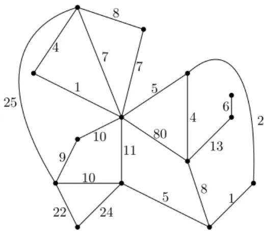
Bien évidemment, de nos jours il existe des algorithmes bien plus sophistiqués. Prenons un exemple plus avancé que la multiplication de deux nombres. Étant donné une carte et la longueur de chaque section de route, on souhaite calculer le plus court chemin entre deux points. Comme le problème est cette fois plus compliqué, et comme nous sommes de bons scientifiques, une bonne idée serait d’abstraire ce prob-lème avec un modèle qui encode toutes les informations dont nous avons besoin, et de résoudre le problème sur ce modèle abstrait. Un modèle abstrait nous débar-rasse de la réalité et devient un pure objet mathématique qui ouvre alors les portes vers toutes les mathématiques pour nous aider à le résoudre. Dans ce contexte, un choix naturel pour un modèle serait de dessiner sur un papier blanc un point pour chaque intersection de route, de dessiner une ligne entre toute paire de points reliés par une section de route et d’écrire le long de cette ligne le nombre correspondant à la longueur de la section qu’elle représente. Maintenant en gardant uniquement notre papier blanc contenant des points, des lignes et des valeurs, nous avons toutes les informations nécessaires pour calculer le plus court chemin entre n’importe quelle paire de points. Notez que même si nous n’avons pas donné d’algorithme qui répond à la question posée, nous avons un modèle des données qui encode uniquement ce qui est réellement essentiel. Voir Figure 1.1 pour un exemple d’un tel modèle. Étant donné un modèle qui contient toutes les données utiles pour notre problème, que pouvons nous dire dessus et comment utiliser ses propriétés intéressantes pour nous aider à fournir une solution à notre question? C’est ce genre de questions qui définit en grande partie l’Informatique Théorique. D’un côté, extraire les propriétés mathé-matiques des modèles, et de l’autre essayer d’utiliser ces propriétés pour développer des algorithmes sophistiqués. Bien sûr, n’importe laquelle de ces branches est un do-maine à part entière des Mathématiques et de l’Informatique. Dans cette thèse, je vais exposer un état de l’art et des résultats nouveaux concernant des problèmes liés à ces deux branches.
Maintenant que nous savons tous ce vers quoi nous souhaitons aller, soyons plus formel vis à vis de ces concepts. Le modèle présenté plus haut est appelé un graphe. Chaque point est appelé un sommetet chaque ligne entre deux sommets, droite ou non cela n’a pas d’importance, est appelée une arête. Deux sommets liés par une arête sont ditadjacents. Unvoisin d’un sommet v est n’importe quel sommet u qui est adjacent à v. Ledegréd’un sommet est le nombre de voisins qu’il a. Notez qu’un
10 5 1 2 9 10 4 8 24 22 80 13 11
Figure 1.1: An example of a map model.
graphe n’est pas un modèle géométrique, dans le sense où nous n’avons pas de co-ordonnées sur les sommets, et les arêtes détiennent uniquement l’information si oui ou non deux sommets sont adjacents. Les graphes sont des outils très puissants per-mettant de modéliser de nombreux problèmes, du plus théorique au plus appliqué. Nous allons donner un aperçu de deux problèmes canoniques de théorie des graphes en lien direct avec plusieurs résultats présentés dans ce manuscrit.
Supposons que l’on nous fournisse un ensemble de produits chimique que nous devons stocker dans des entrepôts. Certains d’entre eux ne peuvent pas être stockés ensemble sans prendre le risque de générer une dangereuse réaction chimique. Ou-vrir un entrepôt chimique est très onéreux. Nous souhaitons donc minimiser le nom-bre d’entrepôt à ouvrir. Nous pouvons modéliser ce problème de la manière suivante. Construisons un graphe où chaque sommet correspond à un produit chimique et pour chaque paire de sommets, mettons une arête si et seulement si les produits sont in-compatibles. La traduction de notre but, qui est de minimiser le nombre d’entrepôts, peut être formulée de la manière suivante. Nous voulons attribuer à chaque som-met une couleur tel que pour toute paire de somsom-mets adjacents les couleurs soient différentes, et nous souhaitons minimiser le nombre de couleurs utilisées. À la fin de notre procédé, le nombre de couleurs est le nombre d’entrepôts à ouvrir et une couleur est équivalente à un type d’entrepôt où tous les sommets de cette couleur seront stockés. Voir Figure 1.2 pour un exemple.
Le problème de coloration peut être énoncé de la manière suivante. Pour tout en-tier k ≥ 1, une k-coloration d’un graphe G est une affection d’au plus k couleurs aux sommets de G. Plus formellement, c’est une fonction c : V(G) → {1, . . . , k}. Une k-coloration propre est une k-k-coloration satisfaisant c(u) 6=c(v)pour toute paire de som-mets adjacents u et v. Un graphe est dit k-colorable si il admet une k-coloration propre. Il est alors naturel de définir le nombre minimum de couleurs nécessaires pour col-orer proprement le graphe. Le nombre chromatique d’un graphe G, noté χ(G), est le plus petit entier k tel que G soit k-colorable. Donc, pour résoudre notre problème de produits chimique de manière optimale, nous devons trouver le nombre chromatique
Figure 1.2: Example of an optimal coloring. 12 11 2 15 2 7 3
Figure 1.3: Example of an optimal set S. Picked vertices are circled in purple.
de notre modèle.
Le deuxième problème classique qui est étudié dans ce manuscrit peut être énoncé d’un point de vue pratique de la manière suivante. Supposons que nous ayons un ensemble possible d’emplacements où nous pouvons ouvrir un restaurant de notre chaîne. Bien sûr, on ne peut pas ouvrir deux restaurants trop proches l’un de l’autre, ce qui aurait pour effet de diviser la clientèle. Chaque emplacement a un bénéfice estimé. Nous souhaitons ouvrir des restaurants tel que le profit soit maximiser tout en respectant la contrainte que deux restaurants ne peuvent pas être trop proches. On peut modéliser cela par un graphe. Pour chaque emplacement sur notre carte, met-tons un sommet et associons à chaque sommet le nombre représentant son bénéfice estimé. Mettons une arête entre deux emplacements (qui sont maintenant des som-mets) dès qu’ils sont trop proches. Ce que l’on souhaite trouver maintenant est un ensemble de sommets S dans notre graphe tel que tous les sommets de S soient deux à deux non-adjacents et qui maximise la somme des profits estimés sur tous les som-mets de S. Voir Figure 1.3 pour un exemple. Nous allons expliquer maintenant ce problème en des termes de théorie des graphes.
Un ensemble indépendant est un sous-ensemble de sommets S⊆V(G)deux à deux non-adjacents. Le cardinal maximum d’un ensemble indépendant d’un graphe G est noté
α(G). Le problème d’Ensemble Indépendant Maximum est le problème consistant à
trou-ver l’ensemble indépendant de cardinal maximum pour un graphe donné. Soit G un graphe, la version pondérée de ce problème est définie par une fonction de poids sur les sommets de G, w : V(G) → Q qui attribue à chaque sommet v un poids w(v).
imum sont tous deux des problèmes difficiles. Mais que veut dire exactement diffi-cile dans notre contexte? Si vous essayez de trouver une solution optimale à l’un des problèmes précédents sur un graphe avec plus de trente sommets, vous allez probablement passer au moins quelques heures pour trouver la bonne solution. En Informatique Théorique, il y a une classification des problèmes en fonction de leur difficulté. C’est une notion très importante en Informatique car cela peut donner une idée si oui ou non un problème spécifique peut être résolu efficacement sur un ordi-nateur. Un problème est ditdécidable en temps polynomialsi étant donné une entrée de taille n, le nombre d’opérations élémentaires nécessaires1pour trouver une solu-tion est borné par un polynôme en n. La classe de tous les problèmes décidables en temps polynomial est notéP. Par exemple, calculer le plus court chemin entre deux sommets u et v est un problème qui est dans la classe P.
D’un autre côté, il y a des problèmes pour lesquels une solution peut être vérifiée en temps polynomial mais pour lesquels il n’y a pas, à l’heure actuelle, d’algorithme polynomial capable d’en trouver une solution. Par exemple, étant donné un graphe, est-il possible de colorer proprement ses sommets en utilisant au plus k couleurs? Vérifier si une solution donnée est valide est facile, cependant dans le cas général, nous n’avons pas d’algorithme polynomial permettant de résoudre ce problème. Le problème de satisfaisabilité est un problème canonique pour lequel on ne sait pas si il existe un algorithme polynomial mais une solution peut être vérifiée rapidement. Ce problème, noté SAT, est un problème de décision qui demande si il existe une interprétation d’un ensemble de variables booléennes qui satisfait une expression booléenne donnée. Nous n’irons pas plus loin dans les détails de ce problème, mais il est important de retenir que ce problème est standard et nous ne savons pas si un jour nous pourrons le résoudre de manière efficace ou non. La classe de problèmes qui sont au moins aussi difficile2que le problème SAT est appelée la classe des prob-lèmes NP-Difficiles. De plus, la classe des probprob-lèmes NP-Difficiles et pour lesquels il est possible de vérifier une solution en temps polynomial est appelée la classe des problèmes Complets. Cook en 1971[21] prouva que le problème SAT est NP-Complet et que tout autre problème dans NP peut être réduit au problème SAT en temps polynomial. Le problème de k-coloration est NP-Complet et le problème qui consiste à trouver un ensemble indépendant de poids au moins k est également NP-Complet. En d’autres termes, ces problèmes sont difficiles. Dans ce manuscrit nous présentons des avancées liées au problème de coloration, au problème d’indépendant de poids maximum et la réfutation d’une conjecture de théorie des graphes en lien 1Une opération élémentaire peut être une opération arithmétique, ou vérifier si deux sommets sont adjacents, etc . . .
2Plus formellement, un problème est NP-Difficile si l’on peut transformer en temps polynomial une instance de SAT en une instance de notre problème.
avec les cliques et les ensembles indépendants.
Les algorithmes avancés sur des problèmes difficiles sont possibles grâce à la con-naissance de la structure des données que nous avons en entrée. Par exemple, trouver l’ensemble indépendant de poids maximum peut être fait en temps polynomial dans des classes de graphes particulière en utilisant les connaissances que nous avons sur leurs structures. D’un autre côté, en ne sachant rien de spécial sur la structure des graphes en entrée, il est peu probable pour que l’on soit capable de fournir un al-gorithme efficace pour ce problème. Donc, en théorie des graphes, décrire la struc-ture des objets que l’on manipule est d’une importance capitale et est un domaine de la théorie des graphes à part entière. La théorie structurelle des graphes a pour but de prouver des théorèmes décrivant les propriétés des graphes. Par exemple, le théorème de Kuratowski [62] décrit complètement lorsqu’il est possible de dessiner un graphe sur le plan sans croisement d’arête. Même si ceci est considéré comme un travail purement théorique, l’impacte que ce genre de résultats a sur des prob-lèmes plus appliqués de théorie des graphes est très important. Dans le Chapitre 4 et Chapitre 6 nous traitons, respectivement, d’une généralisation du problème de col-oration et d’une conjecture lié à des graphes particuliers. Les résultats présentés dans ces deux chapitres ne sont pas d’une nature algorithmique. Ils sont théoriques et améliore la connaissance autour de certaines classes de graphes.
1.1 Contenu du manuscrit
Nous allons donner un aperçu de ce qui est présenté dans ce manuscrit. Les sujets principaux sont la coloration, la coloration par liste, les ensemble indépendant de poids maximum et les graphes normaux.
Le Chapitre 3 est dédié au problème de k-coloration dans les graphes. Nous com-mençons par une brève histoire de la coloration de graphe dans la Section 3.1 et présentons quelques résultats connus concernant une classe de graphes très impor-tante, les graphes parfaits, qui ont un lien très étroit avec le problème de coloration. Puis nous expliquons pourquoi les classes de graphes interdisant des chemins comme sous-graphes induits (les graphes P`-free) sont importants pour le problème de
k-coloration et présentons un résumé des résultats marquant concernant la k-k-coloration des graphes P`-free. Ensuite, nous présentons dans la Section 3.2 la structure des
graphes (P6, bull)-free. Enfin, nous exposons dans la Section 3.3 un algorithme poly-nomial pour la 4-coloration des graphes (P6, bull)-free et pour la k-coloration des graphes (P6, bull, gem)-free.
Dans le Chapitre 4 nous nous intéressons au problème de coloration par liste, qui est une généralisation du problème de coloration. Dans la Section 4.1 nous expliquons comment le problème de coloration peut être généralisé au problème de coloration par liste et pourquoi la classe des graphes sans griffe est importante pour ce problème. En Section 4.2 nous décrivons la structure des graphes parfaits sans griffe. Nous util-isons cette description pour prouver, en Section 4.3, que n’importe quel graphe
par-structurelle des graphes sans taureau que nous utiliserons pour nos algorithmes. Fi-nalement, les sections 5.3 et 5.4 sont dédiées à la présentation d’un algorithme poly-nomial pour le problème d’indépendant de poids maximum dans les graphes (P6, bull)-free et (P7, bull)-free. Les techniques utilisées en Section 5.3 et Section 5.4 sont différentes.
Le Chapitre 6 traite de la réfutation de la conjecture des graphes normaux. La Sec-tion 6.1 commence par décrire l’origine des graphes normaux, expose le contexte et donne un aperçu de ce qui est connu vis à vis de cette classe de graphes. Dans la Sec-tion 6.2 nous décrivons la philosophie de notre outils principal, la Méthode Probabiliste, et fournissons également un exemple d’utilisation de cette méthode en explicitant la preuve d’un célèbre théorème d’Erd˝os. Enfin, en Section 6.3 nous décrivons la struc-ture de notre graphe aléatoire et donnons la preuve de notre théorème faisant appel à un lemma clef dont la preuve est décrite en Section 6.4.
2.1 Context
The notion of counting elements appeared in the story of humanity naturally. As early as 3400 BC, historians have proof that the Sumerians in Mesopotamia devel-oped a numeral system and the concept of weights and measures. From this day, and maybe even earlier, humans continued to develop the concept of counting things, which eventually led to more abstract notions that now fall under what we call Math-ematics. As Mathematics evolved, more sophisticated and complex notions arose. One fundamental one is Arithmetic, that everybody still uses intensively for the day to day life. For a human mind, calculating simple arithmetic operations can be done in a few seconds, for instance, the sum of two small numbers. But as soon as more data is involved, even the simplest operations can take more time. Calculating the sum of a hundred numbers, even though each step is easy, can take several dozen of seconds. As human society grew, the need to calculate larger things emerged. Several tools were manufactured to help deal with such a task. For example, the creation of the abacus is estimated between 2700 and 2300 BC. Of course what our ancestor even-tually had in mind is the great following question: can it be automated? The idea to make machines calculate automatically can have tremendous impact on human life for the following reasons. If the machine calculating process can be done such that no mistake can ever happens, it means that a machine would never be wrong. In addi-tion, if a machine can calculate with great speed, it can give the right answer every time way faster than what a human could do. To get a grasp at how the most ad-vanced computers are good at calculating nowadays, here is a simple fact. A floating point operation is a calculation that involves at least two real numbers (a number that can be written with a comma, such as 1.567). For instance, multiplying 1.545 with 143.75482 is considered as a floating point operation. Even the swiftest mind needs at least a second to compute the previous operation. The best super computer registered as of today is capable of doing 93, 000, 000, 000, 000, 000 floating point operations per
second! However, even though this is an incredible performance, multiplying
bers alone, even at great speed, is not sufficient to send rockets into space, to compute a shortest path on a GPS, or to control an industry process line. What a computer needs to use its calculating speed at maximum power is a series of operations that it needs to follow step by step. This is what is called an algorithm. Given data as an input, a computer following an algorithm will apply the rules contained in the algo-rithm to the data and give the result as an output. For instance, “given two numbers x and y, multiply x and y and give the result”, is a simple example of what is an algorithm.
Of course nowadays there exist very deep and sophisticated algorithms. Let us pick a more advanced example than multiplying two numbers. Given a map and the length of every road section, we would like to compute the shortest path between two points. Since the problem here is more complicated, and as we are good scientists, a good idea would be to abstract this problem with a model that encodes all the infor-mation we need, and then solve the problem on the abstract model. An abstract model rids us of the reality and becomes a pure mathematical object, which then opens the door to all of mathematics to help us solve the problem. In this context, a natural choice for a model would be to draw a point for every intersection of roads on a blank sheet of paper, draw a line between every pair of points connected with a road, and finally on every line, write the number corresponding to the length of the road sec-tion it represents. Now we can only keep our blank sheet of paper and we have all the information we need to compute a shortest path between any pair of points. Note that even though we didn’t give any algorithm to answer the question, we provided a model of the data that encodes only what is really needed. See Figure 2.1 for an example of such a model. Given a model that holds all the interesting data of our problem, what can we say about it and how can we use any interesting fact to help us solve it? This is for the most part, what Theoretical Computer Science is about. On the one hand, extract properties from mathematical models, and on the other hand, try to use those properties to develop clever algorithms. Of course, any of those two branches is a whole field of Mathematics/Computer Science of its own. In this thesis, I am going to give an overview and results related to those two branches.
Now that we all know what we are aiming for, let us get more formal on those concepts. The model presented above is called a graph. Each point is called avertex
and any line between two vertices, straight or not, it does not matter, is called anedge. Two vertices linked by an edge are called adjacent. Theneighborof a vertex v is any vertex u that is adjacent to v. Thedegreeof a vertex is the number of neighbors it has. Note that a graph is not a geometric model, in the sense that we do not have coordi-nates on vertices, and edges are only there to keep the information whether or not two vertices are adjacent. Graphs are very powerful tools able to model many different problem, from the most theoretic to the most applied ones. We will give an overview of two canonical graph theoretic problems on which several results presented in this manuscript are based.
Assume that we are given a set of chemical products that we need to store in warehouses. Some of them cannot be stored in the same warehouse without taking the risk of seeing a dangerous chemical reaction happening. Opening a chemical
10 5 1 2 9 10 4 8 24 22 80 13 11
Figure 2.1: An example of a map model.
Figure 2.2: Example of an optimal coloring.
warehouse is very expensive, so we want to minimize the number of warehouses that needs to be opened. We can model this problem with the following. Construct a graph where each vertex correspond to a chemical product, and for any pair of vertices, put an edge if and only if the products are incompatible. Now the translation of our goal, which is to minimize the number of warehouses, can be put as follows. On each vertex we assign a color such that any pair of adjacent vertices have a different color, and we want to minimize the number of used colors. In the end, the number of colors is the number of warehouses we need to open, and a color is equivalent to a type of warehouse where all vertices of this specific color will be stored. See Figure 2.2 for an example.
The coloring problem can be stated as follows. For any integer k ≥ 1, a k-coloring of a graph G is an assignment of at most k colors to the vertices of G. More formally it is a mapping c : V(G) → {1, . . . , k}. A proper k-coloring is a k-coloring satisfying c(u) 6=c(v)for any two adjacent vertices u and v. A graph is said to be k-colorable if it admits a proper k-coloring. It is then natural to define the minimum number of colors needed to properly color the graph. The chromatic number of a graph G, denoted by
χ(G), is the smallest integer k such that G is k-colorable. Hence, to solve our chemical
products problem optimally, we need to find the chromatic number of our model. The second classical problem that is studied in this manuscript can be stated in a practical way as follows. Assume that we are given a set of possible locations where
12 11
2
15
2 7
3
Figure 2.3: Example of an optimal set S. Picked vertices are circled in purple.
we can open one restaurant of our restaurant chain. Of course we cannot open two restaurants too close to each other, this would only split the customer mass. Each of the locations has an estimated benefit. We want to open restaurants such that it maximizes our profit while satisfying the constraint that no two restaurants can be too close. We can model this by a graph. For every location on our map, put a vertex and associate with each vertex a number representing its estimated profit. Put an edge between two locations (which are now vertices) whenever they are too close to each other. What we want to do now is to find a set of vertices S in our graph such that all vertices in S are pairwise non-adjacent and that maximizes the sum of the estimated profit on all vertices of S. See Figure 2.3 for an example. Let us explain in a graph theoretical way what this optimization problem is.
A stable set is a subset of vertices S ⊆ V(G)such that any two vertices in S are non-adjacent. The stability number of a graph G, denoted by α(G), is the maximum cardinality of a stable set contained in G. The Maximum Stable Set Problem, shortened MSS, is the problem of finding the stable set of maximum cardinality in a given graph. Let G be a graph, the weighted version of this problem is defined by a weight function on the vertices of G, w : V(G) → Q that assigns to each vertex v a weight w(v). The Maximum Weight Stable Set Problem, shortened MWSS, is now to find the stable set of maximum weight, that we denote by αw(G). Note that if w(v) =1 for every v ∈V(G), this is equivalent to the non weighted version.
The graph coloring problem, and the Maximum Stable Set Problem are both hard problems. But what does hard mean exactly in our context? If you try to find an optimal solution to one of the problems stated above on a graph with more than thirty vertices, you might end up spending a few hours to find the correct solution. In Theoretical Computer Science, there is a classification of problems according to their difficulty. This is a very important concept in Computer Science since it can give an idea on whether or not a specific problem might be solved efficiently on a computer. A problem is said to bepolynomial-time solvableif given an input of size n, the number of basic operations1needed to find a solution is bounded by a polynomial in n. The class
1A basic operation can either be an arithmetic operation or checking if two vertices are adjacent, etc . . .
vertices by using no more than k colors? Verifying a given solution is easy, however in the general case, we do not have a polynomial-time algorithm that can solve this problem. The satisfiability problem is a canonical problem for which we do not know if there exists a polynomial-time algorithm that can solve it but a given solution can be checked quickly. This problem, shortened asSAT, is a decision problem which asks if there exists an interpretation of a set of boolean variables that satisfies a given boolean formula. We will not go deeper into the details on this problem, but what is important to remember is that this problem is the standard problem for which we do not know yet if one day we will be able to solve it efficiently. The class of problems that are at least as hard2as the SAT problem is called the NP-Hardclass. Moreover, the class of problems that are NP-Hard and for which it is possible to check in polynomial time if a given solution is valid is called theNP-Completeclass. Cook in 1971 [21], proved that the SAT problem is NP-Complete and that for any other problem in NP, there exists a polynomial reduction to the SAT problem. The k-coloring problem is NP-Complete and the problem of finding a stable set of weight at least k is also NP-Complete. In other words, these problems are difficult. In this manuscript we will present some advances concerning coloring problems, the MWSS problem and a disproof of a graph theory conjecture related to clique and stable sets.
Advanced algorithms on difficult problems are only possible thanks to the knowl-edge of the data structure we have in input. For example, computing the maximum-weight stable set can be done efficiently in specific classes of graphs thanks to the precise structure of these classes. On the other hand, when we do not know anything on the structure of the graph we have in input, it is unlikely that we will be able to produce an efficient algorithm for this problem. Hence, in graph theory, describing the structure of the object we handle is very important and is a subfield of its own. Structural graph theory aims at proving theorems describing properties of graphs. For example, the theorem of Kuratowski [62] fully describes when it is possible to draw a graph on the plane without any edge crossing. Even though this can be con-sidered a purely theoretical work, it has a great impact on more applied graph theory problems. In Chapter 4 and Chapter 6 we deal with respectively, a generalization of the coloring problem and a conjecture linked to a specific graph class. The results presented in these two chapters are not of an algorithmic aspect. They are theoretical and improve the knowledge around two specific classes of graphs.
2More formally, a problem is NP-Hard if one can transform in polynomial time an instance of SAT to an instance of our problem.
2.2 Outline of the manuscript
We will give a general outline of what is present in this manuscript. The main top-ics discussed are coloring, list coloring, maximum-weighted stable set and normal graphs.
Chapter 3 is dedicated to the k-coloring problem in graphs. We start with a short history of graph coloring in Section 3.1 and then present some known results regard-ing a very important graph class, perfect graphs, which is closely linked to the color-ing problem. Then we explain why graph classes forbiddcolor-ing induced paths, P`-free
graphs, are important for the k-coloring problem and present a summary of important results regarding the k-coloring problem in P`-free graphs. Afterwards, we present in
Section 3.2 the structure of (P6,bull)-free graphs. Finally we expose in Section 3.3 a polynomial-time algorithm for the 4-coloring problem in (P6,bull)-free graphs and a polynomial-time algorithm for the k-coloring problem in (P6, bull, gem)-free graphs.
In Chapter 4 we deal with the list coloring problem, which is a generalization of the coloring problem. In Section 4.1 we explain how the coloring problem can be generalized to the list coloring problem and why the class of claw-free graphs is important for this problem. Then in Section 4.2 we describe the structure of claw-free perfect graphs. We use these descriptions to prove in Section 4.3 that any claw-free perfect graph with clique number bounded by 4 has its chromatic number equal to its choice number.
Chapter 5 is dedicated to the Maximum Weight Stable Set problem. Section 5.1 describes the context and why P`-free graphs are interesting regarding this problem.
Then in Section 5.2 we give structure properties of bull-free graphs that will be used in our algorithms. Finally, Section 5.3 and 5.4 are dedicated to the description of a polynomial-time algorithm for the MWSS problem in respectively (P6, bull)-free graphs and (P7, bull)-free graphs. The techniques used in Section 5.3 and Section 5.4 are different.
Chapter 6 deals with a disproof of the Normal Graph Conjecture. First, in Sec-tion 6.1 we start by describing the origins of normal graphs and expose the context and what is known around this specific graph class. In Section 6.2 we describe the philosophy of our main tool used in our disproof, the Probabilistic Method, and also provide a pedagogical example of how it was used in a famous proof of Erd˝os. Fi-nally in Section 6.3 we describe the structure of our random graph and in Section 6.4 provide the proof of our key lemma.
2.3 Definitions
We will define in this subsection classical elementary graph theoretic concepts. A finite simplegraph, denoted byG = (V, E), is an ordered pair consisting of a finite set V, called the vertices, and E, the set of edges which are 2-element subsets of V. An edge{u, v}is also denoted by uv. To refer specifically to the set of vertices
The maximum degree of a graph G, denoted by ∆(G), is the maximum degree among all vertices of G. The complement of a graph G, denoted by G, refers to the graph on the same vertex set and with edge set(V(2G)) \E(G). Theclique number of a graph G, denoted byω(G), is the maximum cardinality of aclique, contained in G,
which is a subset K⊆V(G)of vertices such that any two vertices in K are adjacent. A clique is also called acomplete graphand is denoted byKnwhere n≥1 is the number of vertices. The complete graph on three vertices, K3, is also called atriangle. Astable
setis a subset of vertices S ⊆ V(G)such that any two vertices in S are non-adjacent.
The stability numberof a graph G, denoted by α(G), is the maximum cardinality of
a stable set contained in G. Given a graph G, theinduced subgraph H on the vertex set S ⊆ V(G), denoted by G[S]is the graph on vertex set S and whose edges set is E(H) = {uv∈E(G) | u, v∈ S}. Given two graphs G and G0, we say that G is isomor-phicto G0 if there exists a bijection f from V(G)to V(G0)such that any two vertices u and v of G are adjacent in G if and only if f(u)and f(v)are adjacent in G0. Given a familyH of graphs, a graph G is said to beH-freeif no induced subgraph of G is isomorphic to a member of H. When H has only one element H, we say that G is
H-free.
2.4 Preliminaries
Modular decomposition
We say that a vertex v iscompleteto S if v is adjacent to every vertex in S, and that v
isanticompleteto S if v has no neighbor in S. For two sets S, T⊆ V(G)we say that S
is complete to T if every vertex of S is adjacent to every vertex of T, and we say that S is anticomplete to T if no vertex of S is adjacent to any vertex of T. Ahomogeneous setis a set S ⊆ V(G)such that for every vertex v in V(G) \S, either v is complete to S or anticomplete to S, see Figure 2.4. A homogeneous set is said to be proper if it contains at least two vertices and is different from V(G). Aprime graphis a graph that has no proper homogeneous set. Amodule3 is a homogeneous set S such that every homogeneous set S0 satisfies either S0 ⊆S or S⊆S0or S∩S0 = ∅. In particular V(G)
is a module and every singleton{v} (v ∈ V(G)) is a module. Given a graph G and a partition P of its vertex set where each partition class is a module of G, thequotient
graph, denoted byG/Pis defined as the subgraph of G induced by picking one vertex
from each partition class. The theory of modular decomposition (the study of the
3Note that in the literature one might find a different, but still close, definition of what is a module and a homogeneous set.
S
A B
Figure 2.4: Homogeneous set S, with A complete to S and B anticomplete to S.
modules of a graph) is a rich one, starting from the seminal work of Gallai [34]. We mention here only the results we will use. A subset of vertices S⊆V(G)is amaximal
moduleif S6=V(G)and there is no module S0such that S S0 V(G).
• Any graph G has at most 2|V(G)|modules, and they can be produced by an algorithm of time complexity O(|V(G)| + |E(G)|)[89].
• If both G and G are connected, then G has at least four maximal modules and they form a partition of V(G)(called a modular partition), and every homoge-neous set of G different from V(G)is included in a maximal module; moreover, the induced subgraph G0 of G obtained by picking one vertex from each maxi-mal module of G is a prime graph.
A homogeneous set is a generalization of a connected component in the sense that, in the connected component, every vertex has the same set of non-neighbors outside of the component. In a homogeneous set, every vertex has the same set of non-neighbors and neighbors outside of the homogeneous set.
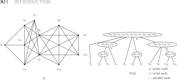
Gallai defined a recursive algorithm to compute the modular decomposition of any graph G. This algorithm takes any graph G in input and outputs the modular decomposition tree, denoted by T(G), which totally encodes the modular decompo-sition. A modular decomposition tree contains three types of nodes. Prime nodes, series nodes and parallel nodes. A prime node represents the fact that the graph G is connected and so is its complement. It means that we can find a modular parti-tion of its vertex set P such that the quotient graph G/P is a prime graph. A serial node implies that the quotient graph induced by the label of its children is a complete graph. Finally, a parallel node implies that the quotient graph induced by the label of its children is a stable set. More formally, the recursive algorithmAdefined by Gallai is described in Algorithm 1.
3: return V(G)
4: else if Gis disconnected then
5: partition G into components M1, . . . , Mk 6: create a parallel node R with label V(G) 7: else if Gis disconnected then
8: partition G into co-components M1, . . . , Mk 9: create a serial node R with label V(G) 10: else
11: partition G into maximal modules M1, . . . , Mk 12: create a prime node R with label V(G)
13: end if
14: for all i∈ {1, . . . , k}do
15: set the nodeA(G[Mi]) as child of R
16: end for
return R
17: end procedure
This algorithm produces the modular decomposition tree of the graph G. In other words, it is a tree which totally encodes the relation (full adjacency or full non-adjacency) between any pair of modules of G and recursively on any subgraph of G induced by a module. See Figure 2.5 for an example of a modular decomposition.
Clique-width
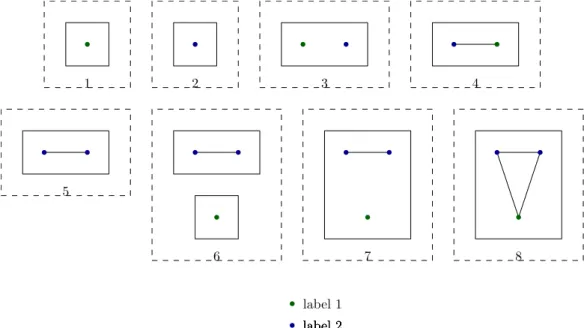
Informally, the clique-width is an integer which measures the complexity of construct-ing G through a sequence of certain operations. More precisely, the clique-width of a graph G, denoted by cw(G), first introduced in [23], is defined as the minimum number of labels needed to construct G by using the following four operations (see Figure 2.6 for an example):
• Create a vertex v labeled by integer i.
• Make the disjoint union of two labeled graphs.
• Join by an edge all vertices with label i to all vertices with label j for two labels i6= j.
• Relabel all vertices of label i by label j.
A c-expression for a graph G of clique-width c is a sequence of the above four
v1 v2 v3 v4 v6 v7 v8 v10 v9 v11 G v1, v2, v3, v4, v5, v6, v7, v8, v9, v10, v11 v1 v2 v3 v4 v5 v6 v7 v8 v9 v10 v11 v2, v3, v4 v2, v3 v6, v7 v8, v9, v10, v11 v10, v11 T (G) p s // // // s p : prime node s : serial node //: parallel node
Figure 2.5: A graph G and its modular decomposition tree T(G).
a graph parameter that has been widely studied. A famous result involves the class of P4-free graphs, also known as co-graphs. In fact, co-graphs can be defined as the graphs having a clique-width of at most 2, as proved in [25]. It is shown in [32] that it is NP-hard to compute the clique-width of a graph G. On the other hand Oum and Seymour [80], provide an algorithm that, given a graph G and a fixed integer c, outputs a c0-expression in O(n9log n), where c0 = 23c+2−1 or a witness that G has clique-width at least c+1. This was later improved by Oum [79] with a complexity ofO(n3)where c0 =8c−1. Courcelle, Makowsky and Rotics proved a meta-theorem which has been used in several occasions to prove the existence of polynomial-time algorithm deciding the k-coloring problem or solving the maximum-weight stable set in certain classes of graphs. They proved that if a class of graph has bounded clique-width c, and for any graph in this class it is possible to find a c-expression in at most f(G)computational steps, then it is possible to find the maximum-weight stable set or decide the k-colorability of G for fixed k, in at most f(G)computational steps. This result is incredibly useful as, in certain cases, it basically narrows down the problem to only showing that a certain class of graphs has bounded clique-width. More formally, their theorem is as follows.
THEOREM2.1[24]
If a class of graphsC has bounded clique-width c, and there is a polynomial f such that for every graph G inCwith n vertices and m edges a c-expression can be found in timeO(f(n, m)), then for fixed k the k-coloring problem or the MWSS problem can be solved in timeO(f(n, m))for every graph G inC.
Moreover, in order to upper bound the clique-width of a graph G, it suffices to consider only the prime induced subgraphs of G.
THEOREM2.2[24, 25]
The clique-width of a graph is the maximum of the clique-width of its prime induced subgraphs.
1 2 3 4 5 6 7 8 label 1 label 2 label 2 label 2
3.1 Context and motivations
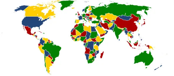
In 1852, Francis Guthrie, a South African mathematician and botanist, while coloring a map of the counties of England in a way such that no two counties sharing a border would receive the same color (see Figure 3.1), noticed in his example that four colors were required. He conjectured from this in 1852 that four colors would be sufficient to color any map as described above. This map coloring problem is the origin of graph coloring. In fact, this exact problem can be seen as a graph coloring problem as follows. For every region of the map put exactly one point in its center. Add an edge between two points whenever the corresponding regions share a border. Finally, ask to assign a color to every vertex such that any two adjacent vertices get different colors. What is the minimum number of color needed to color such a graph? Aplanar
graph is a graph that can be drawn on the plane in such a way that no edges cross
each other. The Four Color Conjecture asked the following, any planar graph can be colored with four colors. This problem, solved since 1977 by Appel and Haken [4], started a very important field in graph theory.
Formally, the coloring problem can be stated as follows. For any integer k ≥ 1, a
k-coloringof a graph G is an assignment of at most k colors to the vertices of G. More
formally it is a mapping c : V(G) → {1, . . . , k}. A proper k-coloring is a k-coloring satisfying c(u) 6= c(v)for any two adjacent vertices u and v. A graph is said to be
k-colorableif it admits a proper k-coloring. It is then natural to define the minimum
number of colors needed to properly color the graph. Thechromatic numberof a graph G, denoted byχ(G), is the smallest integer k such that G is k-colorable.
More generally, graph coloring is a way to formalize a conflict problem in discrete mathematics. Whenever two elements are in conflict, put an edge between them and ask for them to not have the same color. From this setting, natural questions arise. Can we provide the upper and lower bounds on the number of colors needed to respect all the constraints? Is it possible to find a color for every element with a fast algorithm? Rough upper and lower bounds can be obtained easily. Remark that in a clique of size
Figure 3.1: A four coloring of the world map
n, the number of colors needed is n. Hence we obtain the following lower bound on the chromatic number, ω(G) ≤ χ(G). It can be proved by induction on the number
of vertices of G that χ(G) ≤ ∆(G) +1. Pick a vertex v, color G\ {v} by induction and assign to v a color not present in its neighborhood. Hence we obtain the trivial inequality:
ω(G) ≤χ(G) ≤∆(G) +1.
Coloring properly a graph is a way of grouping together vertices that can have the same color. An ideal way of achieving this is to group them in stable sets of maximum size as follows. Pick a stable set of maximum cardinality S and assign to every vertex of S the same color. Delete S from the graph and repeat this until there is no more vertex in the graph. This procedure gives the following other lower bound:
|V(G)|
α(G) ≤χ(G).
It is quite natural to ask how the chromatic number behaves whenever we forbid big sets of pairwise adjacent vertices? It is easy to see that χ(Kn) = n. One could wonder if we can upper bound the chromatic number in terms of the clique number. Even though it might appear to be counter intuitive, this is false. In fact, the chromatic number can be arbitrarily larger than the clique number. Mycielski [75] provided a famous iterative construction of a family of graphs for which (see Figure 3.2 for an example), given any integer k ≥ 1 there exists a graph G in this family such that
ω(G) ≤2 and χ(G) =k.
Mycielski graphs are defined inductively as follows. The first Mycielski graph M1 is the single vertex graph. The second Mycielski graph M2is isomorphic to K2. For k≥2, let V(Mk) = {v1, v2, . . . , vn}where n is the total number of vertices. The k+1th Mycielski graph, Mk+1, is obtained from Mkby doing the following operations:
M
2M
3M
2M
2M
3M
2M
M
33M
4Figure 3.2: The first three Mycielski graphs.
1. Create a copy wi of every vertex viand add an additional vertex z;
2. For each copied vertex wi, put an edge between wiand every neighbor of vi; 3. Add an edge between z and every copied vertex wi.
In other words, Mk+1 is defined by V(Mk+1) = V(Mk) ∪ {w1, . . . , wn, z} and E(Mk+1) =E(Mk) ∪ {wivj |vivj ∈E(Mk)} ∪ {wiz|1≤i≤ n}.
THEOREM3.1[75]
The Mycielski graph Mk, k≥1, is triangle-free and has chromatic number k.
Proof. First, let us show that any Mycielski graph is triangle-free. The first Mycielski graph is the single vertex graph. We proceed by induction on k ≥ 2. The base case, M2, is obviously triangle-free since it is isomorphic to K2. Let us show that Mk+1 is triangle-free. The set W of copied vertices is a stable set of Mk+1. The vertex z is only adjacent to vertices of W. So z is not contained in any triangle. If there is a triangle T in Mk+1, two vertices of T must be in V(Mk) and the third vertex is in W. Let V(T) = {wi, vj, vk}. Since wiis adjacent to vj and vk, it follows from the definition of Mk+1that vi, vj and vk are pairwise adjacent. Hence,{vi, vj, vk}induces a triangle in Mk, a contradiction.
It remains to show that χ(Mk) = k for every k ≥ 1. The first Mycielski graph is the single vertex graph and has chromatic number 1. We proceed by induction on k ≥ 2. The base case M2has chromatic number 2 since it is isomorphic to K2. Let us prove that χ(Mk+1) =k+1. By the induction hypothesis we can color the vertices of V(Mk)with k colors. Now assign to every vertex wi the same color as vi and assign an additional color to z. We obtain that χ(Mk+1) ≤ k+1. It suffices to show now that χ(Mk+1) ≥ k+1. By the induction hypothesis, k different colors appear in Mk. Furthermore, for every color c, there exists a vertex vi of Mk, for some i ∈ {1, . . . , n} depending on c, whose neighborhood in Mkcontains all other k−1 colors, otherwise we could recolor all vertices colored c in Mk and reach a contradiction on the chro-matic number of Mk. Since wi and vi have the same neighborhood in Mk, it follows that k different colors appear in W. Finally, z being adjacent to every vertices of W,
Figure 3.3: Edge coloring example.
needs an additional color. Which gives that χ(Mk+1) ≥ k+1, and the conclusion follows.
One could wonder what specific graphs G are such that ω(G) = χ(G)? And
which graphs G are such that ω(G) < χ(G)? We will discuss this matter in the next
subsection.
Edge coloring of a graph is the analogous version of the vertex coloring, applied to the edge set. Ak-edge-coloringof a graph G is an assignment of k colors to the edges of G, i.e. a mapping C : E(G) → {1, . . . , k}. Similarly, a proper k-edge-coloring is a k-coloring of the edges verifying c(e1) 6=c(e2)for any two edges e1and e2sharing at least one common vertex (see Figure 3.3). Thechromatic indexof a graph G, denoted by χ0(G), is the smallest integer k such that G is k-edge-colorable. A trivial lower
bound on the chromatic index is given by the maximum degree. Given a graph G, ∆(G) ≤ χ0(G). In fact, the chromatic index of simple graphs cannot be far from the
maximum degree. In 1964, Vizing [93] proved the following theorem.
THEOREM3.2[93]
Let G be a simple graph, then χ0(G) ∈ {∆(G),∆(G) +1}.
A multigraph is a graph that can have multiple edges between pair of vertices.
The multiplicityof a graph G, denoted byµ(G)is the maximum number of edges in
any bundle of parallel edges. In a multigraph,the chromatic index is linked to both the maximum degree and the multiplicity. Vizing proved the following more general theorem.
THEOREM3.3[93]
Let G be a multigraph, then∆(G) ≤χ0(G) ≤∆(G) +µ(G).
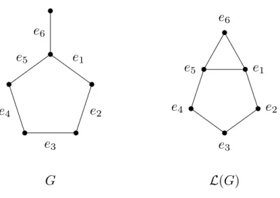
Remark that Theorem 3.2 is a special case of Theorem 3.3 where µ(G) =1. Given a graph H, theline-graphof H, denoted byL(H), is the graph whose vertices are the edges of H and whose edges are the pairs of adjacents edges of H, see Figure 3.4.
e
2e
3e
4G
e
2e
4e
3L(G)
Figure 3.4: A graph G and its line-graph,L(G).Edge coloring can be restated in terms of line-graphs. Given a graph G, coloring the edges of G is equivalent to color the vertices of its line-graphL(G).
3.1.1 Perfect graphs
The birth of perfect graphs takes root in the work of Shannon in [86] concerning zero error capacity of a noisy channel. Aperfect graphis a graph G such that every induced subgraph H of G satisfies χ(H) = ω(H). It is Claude Berge, motivated by the
Shan-non capacity, who initiated the study of perfect graphs. One remarkable moment in the history of perfect graphs is in 1961 when Claude Berge [7] formulated two very famous conjectures (both of them proved by now) about perfect graphs. The first one is the following.
• A graph G is perfect if and only if its complement is perfect.
This was proved by Lovász [65] using the so called Replication Lemma which we restate here for its self interest. Let G be a graph and v a vertex of G. We say that G0is obtained from G by replicating v if G0is obtained by adding a new vertex v0adjacent to v and to all the neighbors of v in G (v0 is also called atwinof v).
LEMMA3.4[65] Replication Lemma
If G is a perfect graph and G0is obtained from G by replicating a vertex v of G, then G0 is perfect.
Let ` ≥ 3 be an integer, the cycle on ` vertices is the graph C` with V(C`) = {v1, . . . , v`}and E(C`) = {v1v2, v2v3, . . . , v`−1v`, v`v1}. Ahole of a graph G is an in-duced subgraph of G which is isomorphic to a cycle on at least four vertices. An
antiholeof a graph G is an induced subgraph of G whose complement is a hole in G.