HAL Id: tel-02513450
https://tel.archives-ouvertes.fr/tel-02513450
Submitted on 20 Mar 2020HAL is a multi-disciplinary open access archive for the deposit and dissemination of sci-entific research documents, whether they are pub-lished or not. The documents may come from teaching and research institutions in France or abroad, or from public or private research centers.
L’archive ouverte pluridisciplinaire HAL, est destinée au dépôt et à la diffusion de documents scientifiques de niveau recherche, publiés ou non, émanant des établissements d’enseignement et de recherche français ou étrangers, des laboratoires publics ou privés.
Nicolas Victorin
To cite this version:
Nicolas Victorin. Multi-component gauge-dependent quantum gases. Quantum Gases [cond-mat.quant-gas]. Université Grenoble Alpes, 2019. English. �NNT : 2019GREAY049�. �tel-02513450�
THÈSE
Pour obtenir le grade de
DOCTEUR DE LA COMMUNAUTE UNIVERSITE
GRENOBLE ALPES
Spécialité : Physique théorique
Arrêté ministériel : 25 mai 2016
Présentée par
Nicolas VICTORIN
Thèse dirigée par Anna Minguzzi, Directeur de Recherche CNRS
préparée au sein du Laboratoire de Physique et de
Modélisation des Milieux Condensés dans l'École Doctorale de Physique
Gaz quantiques à plusieurs
composantes sous champ de jauge
Multi-component gauge-dependent
quantum gases
Thèse soutenue publiquement le 18 octobre 2019, devant le jury composé de :
Monsieur Simone Fratini
Directeur de Recherche, Institut Néel, Président Monsieur Laurent Longchambon
Maitre de conférence, Laboratoire de Physique des Lasers, Examinateur Monsieur Michele Modugno
Professeur, Dpto. De Fisica Teorica e Historia de la Ciencia Facultad de Ciencia y Tecnologia, Rapporteur
Madame Anna Minguzzi
Directeur de Recherche CNRS, Communauté Université Grenoble Alpes, Directeur de Thèse
Multi-component Gauge-Dependent
Quantum Gases
Contents
I Two component ring under gauge fluxes
11
1 Artificial gauge fields with ultra-cold atoms in optical lattices 13
1.1 Optical lattices . . . 13
1.1.1 Bose-Hubbard model . . . 14
1.1.2 Ring shaped lattice . . . 16
1.2 Gauge field . . . 16
1.2.1 Analogy between rotation and magnetic field, persistent currents . . . 17
1.2.2 Magnetism and quantum physics . . . 18
1.2.3 Lattice systems . . . 20
1.3 Peculiarities of one dimensional systems . . . 22
1.3.1 Condensation and coherence properties in 1D . . . 24
2 Mean-field of the double ring 27 2.1 Gross-Pitaevskii equation . . . 27
2.2 The model . . . 28
2.3 Non interacting regime . . . 30
2.3.1 Persistent and chiral currents . . . 32
2.3.2 Infinite system - Variational Ansatz . . . 33
2.4 Mesoscopic effects and commensurability of the flux . . . 34
2.4.1 Vortex configurations on a finite double ring lattice . . . 34
2.4.2 Fate of the single vortex in the Meissner phase . . . 34
2.4.3 Spiral interferograms . . . 37
2.5 Mean-field ground state phase diagram . . . 40
2.5.1 Coupled discrete nonlinear Schrödinger equations (DNLSE) . . . 40
2.5.2 Persistent currents for interacting bosons on the double ring lattice . . 41
3 Bogoliubov excitations 45 3.1 Diagonalization of general quadratic Hamiltonian . . . 46
3.2 Bogoliubov formalism . . . 47
3.2.1 Zero frequency modes . . . 49
3.2.2 Josephson effect . . . 49
3.3 Model and method . . . 52
3.3.2 Dynamical structure factor . . . 54
3.3.3 Static structure factor . . . 56
3.4 Excitation spectrum as a probe of the phases of the two-leg bosonic ring lad-der . . . 56
3.4.1 Meissner phase . . . 57
3.4.2 Biased-ladder phase . . . 60
3.4.3 Vortex Phase . . . 60
3.4.4 Experimental probe of dynamical structure factor . . . 61
3.5 Coherence properties and supersolidity . . . 63
3.5.1 One-body density matrix . . . 63
3.5.2 Static structure factor - probe of solidity . . . 64
3.6 Small ring limit and nature of the excitations . . . 65
3.7 Bogoliubov excitation spectrum for the lowest single-particle branch . . . 66
3.8 Details on the approximation . . . 68
4 Hard-core bosons 71 4.1 Tonks-Girardeau Bose-Fermi mapping . . . 72
4.2 Fragmentation . . . 75
4.3 Fragmented Fermi seas . . . 76
4.3.1 Bose-Fermi mapping . . . 78
4.4 Numerical results . . . 79
4.4.1 Fidelity with respect to fragmented states . . . 79
4.4.2 Currents . . . 81
4.4.3 Current-current correlations . . . 82
4.4.4 Density-density correlations . . . 82
4.4.5 One-body density matrix and momentum distribution . . . 83
5 Quantum fluctuation effects, Luttinger liquid description 91 5.1 Bosonization and Luttinger liquid . . . 91
5.1.1 Correlation functions . . . 92
5.1.2 Sine-Gordon model . . . 93
5.2 Luttinger liquid description of the double ring . . . 95
5.2.1 Derivation of the Luttinger Liquid Hamiltonian of the double ring . . . 95
5.2.2 Meissner-Vortex transition . . . 96
5.2.3 Mode expansion . . . 99
5.2.4 Weak link . . . 101
5.2.5 Current and correlations functions in the vortex phase . . . 102
II Polaritons in honeycomb lattice
109
6 Exciton-Polaritons and the honeycomb lattice 111 6.1 Exciton-polaritons . . . 112Contents
f
6.1.2 The driven-dissipative mean-field Gross-Pitaevskii equation . . . 116
6.1.3 Steady state and bistability . . . 116
6.2 Honeycomb lattice . . . 119
6.2.1 Berry phase . . . 121
6.2.2 Brillouin zone selection . . . 123
6.2.3 Coupling to photonic bath vacuum . . . 124
7 Bogoliubov excitation spectrum of polaritons in honeycomb lattice 127 7.1 Bogoliubov excitation spectrum . . . 127
7.1.1 Stability analysis . . . 131
7.2 Experimental excitation spectrum . . . 132
7.2.1 Experimental realization . . . 133
7.2.2 Retarded Green’s function . . . 134
8 Conclusion and perspectives 137
A Diagonalization of the non interacting Hamiltonian 141
B Numerical method for the solution of the DNLSE 143
C Interference patterns of expanding rings 145
D Rigol’s method for hard-core bosons 147
E Conformal field approach 149
T
HEfirst observation of Bose-Einstein condensation (BEC) in dilute atomic vapors[1] has been a breakthrough both fundamentally, verifying theoretical concept predicted by Bose [2] and Einstein[3] several decades ago, and experimentally, because in order to reach the BEC regime with ultra-cold atoms a temperature of the order of 10−9K
had to be reached revealing the statistical property of quantum particles. Since then, a new field has emerged and experimentalists are able to study this artificial matter in a very clean and controllable way both for bosons and fermions. Interactions between atoms can be long-ranged [4] or short-ranged [1]. In the latter case, the strength of the interac-tion can be tuned using Feshbach resonances. Light-matter interacinterac-tion is the key tool to confine atoms and the shape of the confining potential can now be controlled with very high precision. Such cold-atom systems allows us to explore a whole range of fundamen-tal phenomena that are extremely difficult or impossible to study in real materials, such as Bloch oscillation, Mott-superfluid transition, topology of band structure, orbital mag-netism just to name a few. Specially designed optical lattice experiments are paving the way to study condensed-matter problems where particles are confined into a periodical potential. Recent experimental advances using ultra-cold quantum gases has allow to en-gineer the coupling between different internal states of the atoms, in order to realize syn-thetic gauge fields [5, 6, 7]. The dynamics of the center-of-mass of a neutral atom which moves in a properly designed laser field, is analogue to the dynamics of a charged particle in a magnetic field, on the influence of a Lorentz-like force. The corresponding Aharonov-Bohm phase is related to the Berry’s phase that emerges when the atom adiabatically fol-lows one of the dressed states of the atom-laser interaction [5]. These progresses allow the quantum simulation of a large class of Hamiltonians. Indeed, condensed matter phe-nomena under strong magnetic fields are still intriguing and are at the center of modern research. For instance, topological states of matter are realized in quantum Hall systems, which are insulating in the bulk, but bear conducting edge states [8].
A ladder is the simplest geometry where one can get some insight on two-dimensional quantum systems subjected to a synthetic gauge field [9, 10]. The bosonic linear ladder has been the subject of intense theoretical work. The phase diagram has been established by means of field-theoretical methods [11, 12], and intensive DMRG simulations [13]. Those studies, in addition to common features of Bose-Hubbard models such as super-fluid and Mott insulating phases, revealed new exciting phases of matter induced by the magnetic field: chiral superfluid phases, chiral Mott insulating phases displaying Meissner currents [12, 14] and vortex-Mott insulating phases [15]. In the weakly interacting regime, an additional phase has been predicted [16] a biased ladder phase characterized by an imbalanced population of the bosons between the two legs, explicitly breakingZ2
sym-metry. This phase was shown to be stable in the interacting case, except for a special value of the applied flux, where umklapp processes destabilize it [17]. The dependence of the
Contents
f
critical flux separating Meissner and vortex phase on inter particle interactions has been also studied [18]. In parallel to these theoretical advances, the experimental realization of the bosonic flux ladder has been reported in optical lattices [19] as well as for lattices in synthetic dimensions, both for fermions and bosons [20, 21].
As in the case of cold atoms, exciton-polaritons in semiconductor microcavities are an ideal model system to simulate and engineer condensed matter systems. They allow for the control of the density, the temperature of the sample, and, in the case of lattice sys-tems, the topology of the band structure. It is possible to directly image exciton polaritons thanks to the their photonic component: all the statistical properties of the intracavity polariton field are contained in the far-field of the polariton luminescence [22]. The possi-bility of realizing coupled micropillars thanks to deep etching of a planar structure [23, 24] has opened the way towards the engineering of lattices for polaritons with controlled tun-neling and deep on-site potentials with arbitrary geometry. The honeycomb lattice is one of such intriguing condensed matter system where topological effect arise. One of the most interesting aspect of the honeycomb lattice problem is that its low-energy excita-tions are mass-less, chiral, Dirac particles. This particular dispersion, that is only valid at low energies, mimics the physics of quantum electrodynamics (QED) for mass-less par-ticles except for the fact that in honeycomb lattice the Dirac parpar-ticles move with a speed of sound vS, which is 300 times smaller than the speed of light c. Hence, many of the
un-usual properties of QED such as the Klein paradox [25] can show up in graphene but at much smaller speeds or, identically, energy scales.
In the first part of this thesis, i.e chapters 2, 3, 4 and 5, we consider a system made of two one-dimensional coupled lattice rings subjected to different fluxes in each leg. This specific bosonic ladder corresponds to different boundary conditions with respect to the case of a linear ladder. In particular, this double ring lattice geometry allows to study per-sistent currents in dimension larger than one [26], which shows promising applications for atomtronics developments [27, 28]. We focus on a planar geometry with concentric rings, as could be realized eg with dressed potentials [29], or using co-propagating Laguerre-Gauss beams [30].
The first part of the thesis is organized as follows:
In chapter 1 we introduce some key concepts about cold-atoms experiments focusing on the trapping of atoms by light potential in optical lattices. We also provide some infor-mations about gauge-dependent phenomena by connecting to the notion of Aharonov-Bohm effect. Finally we discuss the peculiarities of bosons in one dimensional systems. Then throughout the next chapters 2, 3, 4 and 5 the theoretical methods employed to de-scribe the model studied in different physical regimes are introduced, and original results are presented.
rings subjected to different fluxes in each leg is derived. After identifying the vortex and Meissner phases, we discuss specific features of the double ring lattice geometry, as the appearance of a vortex in the Meissner phase and parity effect in the vortex phase arising from the commensurability of the total flux. Through a numerical study we then explore the dilute, weak-interacting regime and address the nature of the ground state at mean-field level. In particular we identify known phases [16] such as the Meissner, vortex and biased-ladder phases as well as the effect of commensurability of the total flux. The persis-tent current is shown to be a good observable to identify the different phase of the system. Finally, we propose the spiral interferogram images obtained by interference among the two rings during time of flight expansion as a probe of vortex-carrying phases, specifically adapted to the ring geometry. The results outlined in this chapter can be found in the fol-lowing published article:
Nicolas Victorin, Frank Hekking, and Anna Minguzzi. Bosonic double ring lattice under artificial gauge fields. Phys. Rev. A, 98:053626, Nov 2018
In chapter 3, using both numerical and analytic approaches, we explore the excita-tion spectrum of two one-dimensional coupled lattice rings subjected to different fluxes in each leg. The excitation spectrum in Meissner, biased-ladder and vortex phase is ex-plicitly shown via the dynamical structure factor. We show that the vortex phase has su-persolid properties stemming from the combination of coherence and spatial order. Then the nature of the Bogoliubov modes is studied reveling Josephson oscillation between the two rings. The results outlined in this chapter can be found in the following arxiv article: Nicolas Victorin, Paolo Pedri and Anna Minguzzi. Excitation spectrum and supersolidity of a two-leg bosonic ring ladder. arXiv:1910.06410, Oct 2019
In chapter 4 we explore the regime of infinitely strong interactions on the double ring. We make use of the exact mapping into fermions via the Jordan-Wigner transformation, that is made possible in a peculiar physical regime at strong magnetic flux and weak cou-pling between the rings. Using both analytic and exact diagonalization, fragmentation of the ground-state is explicitly shown ranging from a fragmentation in momentum space at weak interaction to a fragmented Fermi sea at infinite interaction. The regime of frag-mented Fermi sea is then characterized via different physical observables. The results outlined in this chapter can be found in the following published article:
Nicolas Victorin, Tobias Haug, Leong-Chuan Kwek, Luigi Amico, and Anna Minguzzi. Non-classical states in strongly correlated bosonic ring ladders. Phys. Rev.A, 99:033616, Mar 2019.
In chapter 5 we explore the intermediate regime of interactions. Thanks to a mode ex-pansion and re-fermionization approach of the bosonized Hamiltonian of the double ring under gauge flux, we show the peculiarities of finite size periodic boundary condition on the current in the double ring. A rotating barrier is then introduced and we show a gap opening in the spin sector of the energy spectrum. The dynamical structure factor is de-rived revealing the decomposition in spin and charge mode of the excitation spectrum at
Contents
f
low energy. The results outlined in this chapter is the outcome of an on going work. In the second part of this thesis, i.e Chapters 6 and 7, we consider a system of exciton polaritons in honeycomb lattice. Driven by experiment realization of the model in Institut Néel in the group of Maxime Richard, we explore the Bogoliubov excitation spectrum of the model as well as its observation in relation with relevant experimental procedures.
The second part of the thesis is organized as follows:
In chapter 6 we review some key concepts about exciton-polariton in microcavities. Then we study the honeycomb lattice and its low energy properties. We outline the con-cept of Brillouin zone selection mechanism and we provide a new interpretation in terms of dark-state.
In chapter 7 we explore the Bogoliubov excitation spectrum of exciton-polaritons in honeycomb lattice structure. We show that this Bogoliubov spectrum exhibit a instability of the C point of the bistability curve that is usually stable for polariton in microcavities. Superfluid properties below and above the C point arises at momentum away from the momentum of the laser pump that populate one of the Dirac point of the system. Finally we see that the theory derived in this chapter models experimental observation of the ex-citation spectrum of interacting polaritons in honeycomb lattice.
The second part of this thesis is part of an on going work.
List of published and soon to be published work
The original results presented in this thesis have been published in the following articles: (i) Nicolas Victorin, Frank Hekking, and Anna Minguzzi. Bosonic double ring lattice
under artificial gauge fields. Phys. Rev. A, 98:053626, Nov 2018
Subject of part I, chapter 2
(ii) Nicolas Victorin, Tobias Haug, Leong-Chuan Kwek, Luigi Amico, and Anna Minguzzi. Non-classical states in strongly correlated bosonic ring ladders. Phys. Rev.A,
99:033616, Mar 2019.
Subject of part I, chapter 4
(iii) Nicolas Victorin, Paolo Pedri and Anna Minguzzi. Excitation spectrum and supersolidity of a two-leg bosonic ring ladder. arXiv:1910.06410, Oct 2019
Subject of part I, chapter 3
(iv) Nicolas Victorin, Roberta Citro and Anna Minguzzi. Luttinger Liquid description of a two-leg bosonic ring ladder subjected to gauge fluxes. In preparation.
Subject of part I, chapter 5
(v) Petr Stepanov, Nicolas Victorin, Anna Minguzzi and Maxime Richard. Experimental observation of the excitation spectrum of an interacting gas of polariton in
a honeycomb lattice. In preparation.
Part I
Chapter 1
Artificial gauge fields with ultra-cold
atoms in optical lattices
T
HIS chapter will focus on the necessary tools to understand the content of Part I of this manuscript. The relevant concepts of optical lattices, gauge fields and the emerging phenomena of ultra-cold gases placed under those constraints will be in-troduced. Also, the peculiarities of bosonic one dimensional many-body systems will be reviewed. All other necessary concepts will be introduced at the beginning of each forth-coming chapter.1.1 Optical lattices
Using the sensitivity of the electrons of an atom to an oscillating electric field E(r, t ) it is possible to engineer a trapping potential for neutral atoms. Indeed, the interaction be-tween electrons and an electric field made by laser field induce a dipole moment that os-cillates with the imposed laser field, far from resonance reads
di±(t ) = X
j =x,y,z
αi j(ωL)E±j(r, t ) (1.1)
where di±is the ithcomponent of the dipole moment,ωLthe laser frequency andαi j(ωL)
the matrix elements of the complex polarizability tensor characteristic the response of the atoms to the applied electric field. The energy shift is then∆E = d · E and for a fully isotropic response of the medium to applied electric field it is diagonal, i.eαi j= αδi j,
∆E(r,t) = −2Re[α]I(r,t) ∝ I (r, t )
∆ (1.2)
where I (r, t ) is the laser beam intensity and∆ = ωL− ω1is the detuning of the laser
Figure 1.1: Schematic pictures of optical lattice potentials created by counter-propagating lasers: (a) 2D array of quasi-1D tubes and (b) 3D simple cubic lattice. From [32].
that the atoms feel an optical potential created by the spatial pattern of the laser field in-tensity. This technique is widely used for trapping atoms [31]. Upon changing the sign of the detuning∆ it is possible to change the sign of the potential and therefore its attractive or repulsive character.
Optical lattices are formed using light confinement forming periodic intensity pattern thanks to interference of two or more laser beams. The simplest optical lattice can be made with two laser beams with the same wavelength, with paths which are in opposite direction. Their interference creates a 1D periodic intensity pattern of period half their wavelength, of the form
V (x) = V0sin2(k x) (1.3)
with k = 2π/λ, λ being the wavelength of the lasers that form the standing wave and V0
the depth of the optical lattice proportional to the intensity of the laser beam. It is possible then to create complex lattice structures by creating complex interference patterns playing with wavelength, angle, polarization, shape and number of the laser beams.
1.1.1 Bose-Hubbard model
A relevant Hamiltonian for lattice models is the Bose-Hubbard Hamiltonian that is useful to treat a lattice system in tight binding approximation and has proven to be the relevant one to describe bosonic atoms with repulsive interaction in a periodic lattice potential [33]. We will review here its derivation as it will be helpful for the next chapters 2, 3, 4,
1.1. Optical lattices
f
5 and in Part II of this thesis. The Bose-Hubbard Hamiltonian can be derived from the general second quantized form of many-body Hamiltonian
H = Z d rψ†(r)hrψ(r) + Z d r0 Z d rψ†(r)ψ†(r0)Vr,r0ψ(r0)ψ(r), (1.4) where hr is a general differential operator acting on the bosonic field operatorsψ(r)
rep-resenting the kinetic energy and the external potential, and the second term Vr,r0 is the inter-particle interactions. In the specific case of atoms in an optical lattice, hr= −ħ
2
2m52r
+Vlatt(r) + Vext(r) whereVlatt(r) represents the lattice confining potential and Vext(r) an
ex-ternal potential. In typical cold-atom experiments the quantum gas is very dilute, with densities typically ranging from 1013to 1015cm−1. Interactions between atoms are never-theless very important and are well characterized by two-body contact interactions at low energy. The interactions are then described by a single parameter, the s-wave scattering length as, which enters into the contact two-body interaction potential Vr,r0 = g δ(r − r0) where g = 4πħ2as
m . The s-wave scattering length is tunable using Feschbach resonances
[34]. This provides to the cold-atoms experiments a unique playground to study effect of interactions between particles for a large range of interaction strengths. Considering deep lattice potentials, we use a tight-binding approximation that consists in expanding bosonic field operator on the basis of Wannier functions of the lowest band,
ψ(r) = X
i
biw (r − ri), (1.5)
where bi and bi†are respectively the annihilation and creation operators of a particle
lo-calized in the ith lattice site, satisfying bosonic commutation rules hbi, b†j
i
= δi j. This
approximation works also for interacting bosonic gases as long as the typical interaction between particles is not enough to excite the population of higher bands. One then ob-tains the Bose-Hubbard Hamiltonian by taking into account only nearest neighbor hop-ping and contact interactions,
H = −X 〈i , j 〉 ³ Ji jb†ibj+ h.c ´ +U 2 X i ni(ni− 1), (1.6)
where 〈i , j 〉 is restricting the sum to nearest neighbors and ni = b†ibi is the number
op-erator of bosons on each site. The coefficients Ji j is interpreted as the rate of tunneling
between site i to j through the lattice potential barrier and it is given by
Ji j= − Z d rw∗(r − ri) · −ħ 252 r 2m + Vext(r) + Vlatt(r) ¸ w (r − rj). (1.7)
As the Wannier functions are strongly localized in the tight binding approximation, the on-site interaction U is given by
U = g
Z
1.1.2 Ring shaped lattice
The geometry of the lattice that one can consider depends on the intensity pattern formed by the interference of the laser beams. Therefore, a large class of lattices can be consid-ered e.g cylindrical optical lattices[30]. Those lattices can be formed using Laguerre-Gauss beams carrying angular momentum [35, 36], see Fig. 1.2. Another way of forming ring
Figure 1.2: Two rings geometry, formed by two Laguerre-Gauss beams with flux per placket Φ. From [30].
shaped lattice is to use the idea of synthetic dimensions that uses the internal degrees of freedom of the atoms to generate extra transverse dimensions [37].
1.2 Gauge field
In the context of the standard model, gauge theories describe three of the four fundamen-tal forces of nature, electromagnetism U(1), weak SU(2)×U(1) and strong SU(3) forces. These symmetries imply invariance of the Lagrangian and define conserved charges that are linked to the bosons that mediates those forces. In the context of condensed mat-ter, those gauge symmetries are widely used and many-body quantum system subjected to external magnetic fields exhibit rich and intriguing behaviour. Integer and fractional quantum Hall effects are examples of such physical effects, where the transverse trans-port of a 2D system induced by external magnetic field exhibits plateaus corresponding to
1.2. Gauge field
f
an integer or fractional multiple of e2/h [38], e and h being the electron charge and the Planck’s constant, respectively. This effect arises for charged particles with applied mag-netic field but can also be induced by an artificial magmag-netic field on neutral bosonic atoms. Several ways of inducing magnetic like dependence on neutral atoms are possible, to cite a few :
• rotating trapped ultra-cold gases: using to analogy between Lorentz and Coriolis force[39, 40]: with this technique it is possible to create Abelian gauge fields.
• laser induced gauge fields in optical lattices: exploiting properties of laser-assisted tunneling [41] (see Fig. 1.3) it is possible to access the regime of large magnetic field.
Figure 1.3: Laser assisted tunneling is a way of implementing gauge field in optical lattice. Using internal degrees of freedom of the neutral atoms: with this technique it is possible to implement a complex hopping. From [42]
.
1.2.1 Analogy between rotation and magnetic field, persistent currents
Let’s consider a fluid of neutral particles confined in a trap that is rotating at frequencyΩ around the z axis. We show here below that the dynamics of a fluid is equivalent to charged particles subjected to magnetic field. One can link magnetic and rotation frequency in the following way
qB = 2mΩ with Ω = Ωez (1.9)
where q is the charge of the particle and m the mass. The rotation induce a Coriolis force on the fluid that is FC= 2Mv × Ω that is very similar to the Lorentz force acting on charge
particle FL= qv × B. Let’s draw the analogy a little bit deeper by considering the full
quan-tum Hamiltonian problem of the rotating fluid, this time in first quantization. Let’s con-sider a quantum particle of mass m evolving in a one dimensional ring of circumference
L, radius R and rotating defect turning at velocity vθ= veθ
ˆ H (t ) = pˆ 2 θ 2m+ δ(Rθ − v t ) = − ħ2 2mR2∂ 2 θ+ δ(Rθ − v t ) (1.10)
Figure 1.4: Experimentally observed vortex lattice arising from the rotation of a bosonic atomic BEC. The pictures show different configuration of the number of vortices in the sample. Taken from [44].
One can eliminate the time dependence in the Hamiltonian by a unitary transformation ˆ
U (t ) = exp(i Ω ˆLzt /ħ) where ˆLzis the angular momentum operator ˆLz= −i ħ∂θ. The
Hamil-tonian transforms into
ˆ H0= ˆU (t )†H (t ) ˆˆ U (t ) = ħ 2 2mR2¡−iħ∂θ− q Aθ ¢2 + δ(θ) + Vcentr (1.11)
where Vcentr represents the centrifugal effect Vcentr= −12mR2Ω2 and qA = mΩ × ˆr. The
action of the unitary transformation ˆU (t ) is to change the frame of reference of the
sys-tem to the moving frame of angular frequencyΩ so that the momentum of the particle in the moving frame is shifted by the analogue of a magnetic vector potential. The only difference is the centrifugal potential effect, however for a 1D ring this contribution can be considered as a constant shift of the full spectrum so that it will not be relevant. For 2D systems this contribution tends to push the particles away from the center and one cannot have a toy model of orbital magnetism on a neutral gas. To overcome this problem the confining trap is turning at frequency equal to the confinement frequency so that the centrifugal contribution cancel out with the trapping contribution and one can observe 2D gauge dependent physics [5, 43]. This analogy allowed to experimentally access gauge dependent physics and create vortex lattices in BEC experiments [44]. Figure 1.4 shows an example of a vortex lattice.
1.2.2 Magnetism and quantum physics
Continuum case : The Maxwell equation for the magnetic field B in the absence of mag-netic monopoles 5r.B(r) = 0 implies B(r) = 5r× A(r). It shows that the equation is
invari-ant under transformation of the vector potential up to a gradient term a scalar fieldφ(r), meaning that two vector potentials A(r) and A(r)0where A(r)0= A(r) + 5rφ(r) lead to the
same magnetic field. This gauge invariance can be absorbed at the level of the quantum Hamiltonian H = 1 2m Z d rψ†(r)£−iħ 5r−qA(r) ¤2 ψ(r) (1.12)
1.2. Gauge field
f
where q is the charge of the particle, by a redefinition of the momentum operator ˆ
p → ˆp0= −i ħ 5r+q 5rφ(r) (1.13)
or by a change of gauge of the field operators
ψ(r) → ψ(r)0= ˆUψ(r) = ei qħφ(r)ψ(r) (1.14)
This define a U(1) gauge invariance. One important fact is that the invariance of the mag-netic field upon a shift of the vector potential by a gradient term lies on the fact that the space is connected, meaning that closed loop can be deformed continuously into a dot. This will not be the case for a particle evolving in a space where a singularity is present. The Aharonov–Bohm effect [45] is such an example.
The Aharonov-Bohm effect is the sensitivity of the phase of the wave function to the vector potential of the magnetic field. Let’s consider (see Fig.1.5) a charged particle evolv-ing in a plane with a solenoid createvolv-ing a non-zero magnetic field only inside itself. The Hamiltonian describing such a setup is the following
H = ¡ ˆp − qA(r)¢
2m . (1.15)
Outside of the solenoid we have no magnetic field so that 5 × A(r) = B(r) = 0. As we said earlier, the vector potential of the magnetic field can be expressed as the gradient of a scalar field only if the space is simply connected (i.e there is no singularity of the magnetic field). We can only define a vector potential for different path but not enclosing the discon-tinuity. For the two beams of Fig.1.5 we can define such a vector potential that we’ll call AI /I I(r) = 5χI /I I(r) associated to wave functionΨI /I I = e
i
ħqχI /I I(r)Ψ0(r) where the phase
has been absorbed into the wave function andΨ0(r) is wave-function without magnetic
field. The dephasing between the two wave functions at a point r is then
φ =q ħ ¡ χI(r) − χI I(r)¢ = q ħ I CA(r)d r = 2π Φ Φ0 (1.16) whereΦ is flux in the solenoid and Φ0the quantum of flux. Such an effect is remarkable
as the presence of a magnetic field yield a dephasing of the particles circulating around it without encountering it: the particles are affected by the flux of this magnetic field as a direct consequence of the gauge invariance of the quantum theory. This phase is said to be topological as it is not depending on the path chosen.
The persistent current phenomenon arises from the Aharonov-Bohm effect which af-fects the quantum dynamics of charged particles in a multiply-connected geometry [45] (i.e with holes). In condensed-matter physics the study of persistent currents has emerged in the context of metallic rings under magnetic fields at very low temperature. If quantum phase coherence is large compared to the size of the system and thermal fluctuations are
Figure 1.5: Representation of the Aharonov set-up: incoming electrons take two alterna-tive paths around a solenoid. The beam is then recombined and interference is observed. Figure from [46].
weak enough, persistent currents manifest themselves as dissipationless currents even in the absence of any applied voltage [47]. Persistent currents were first observed in solid state superconductors electronic systems subjected to a magnetic field [48].
Mathematically, the persistent current is defined [49] through the Hellman-Feynman the-orem as I = −Φ10〈∂ΦH 〉 = −Φ10∂Φ〈H〉. For a homogeneous system without impurities, the
spectrum is En=¡n −2LπΦ/Φ0
¢2
, where n ∈ Z labels the different angular momentum state. The persistent current is then an oscillating function of period fixed by the quantum of flux Φ0. Impurities will break the rotational invariance and couple the different angular
mo-mentum states of the system. This will introduce a gap between the different energy levels
Encorresponding to momentum n for any value of repulsive interactions (Leggett’s
theo-rem [50]).
We see from Eq.(1.11) that even a moderate concentration of impurities will affect the cur-rent amplitude. Nevertheless, the persistent curcur-rent is stronger than one can think. In-deed, when performing a gauge transformation, ψ(θ) → ei q Aθψ(θ) one removes the Aθ dependence in the Hamiltonian on the price of twisting the boundary condition (ψ(0) =
e2πAθψ(2π)). The persistent current is then seen as a measure of the sensitivity of the spectrum to the twist, so that even in presence of disorder the persistent current does not vanish. This fact has been observed in metallic rings in a disordered environment [51]. Of course, rotating Bose-Einstein condensates made of ultra-cold atoms, being in a su-perfluid state, will exhibit coherence properties analogue to electronic superconducting system and dissipationless flow is likely to occur [52].
1.2.3 Lattice systems
In a lattice two length scales are competing, the inter-site distance a and the magnetic length l =pħ/qB. Their ratio can be expressed as the ratio of the magnetic flux Φ and
1.2. Gauge field
f
the quantum of fluxΦ0. WhenΦ is much smaller than Φ0nothing more is expected than
for the case of a single particle whereas forΦ ≈ Φ0the physics will change drastically and
can create fractal structure in the energy spectrum (Hofstadter butterfly [53]). Artificial materials, such as the ones which can be implemented in cold atoms experiments [6, 7] are able to access those regimes since the inter-site distance can be tuned so that it becomes comparable with the magnetic length. In the tight binding approximation, (see Eq.1.6), we consider the Bose-Hubbard Hamiltonian. For simplicity we will consider a 1D chain
H = −JX l ³ a†l +1al+ h.c ´ . (1.17)
In the presence of a magnetic field perpendicular to the sample, we have to take into ac-count the Aharonov-Bohm phase that is accumulated by a particle from a site l to l0of the lattice φ(l → l0) =q ħ Z rl 0 rl A(rm).d rm (1.18)
At the level of the Bose-Hubbard Hamiltonian this phase can be included via the Peierls substitution [54] in the tunneling coefficient J → Jeiφfor a constant magnetic field. Thus the Hamiltonian reads
H = −JX l ³ a† l +1ale iφ+ h.c´ . (1.19)
2D lattice The situation for a square lattice is analogous. The 2D lattice Bose-Hubbard Hamiltonian is H = −J X m,n ³ am+1,n† am,n+ a†m,n+1am,n+ h.c ´ . (1.20)
Due to the presence of the magnetic field, the hopping is complex due to the Peierls sub-stitution, of phaseφim,n= q Aim,n/ħ at site {m,n} in direction i = {x, y}. So that the
Hamil-tonian transform into
H = −J X m,n ³ eiφm,nx a† m+1,nam,n+ e iφym,na† m,n+1a m,n + h.c´ (1.21)
For a homogeneous magnetic field the flux is fixed and equal for each plaquette (as de-noted byΦ in 1.6), Φ = φxm,n+ φm+1,ny − φxm,n+1− φm,ny and represents the gauge invariant
quantity of the square lattice. All along this thesis we will consider the Landau gauge, un-der which the vector potential is aligned to a certain direction of space x or y. When it is aligned in the x direction, the vector potential is A = (−B y,0,0) and we are in the situation considered by Atala et al in the experiment on bosonic ladders[19] (see Fig. 2.2). In the case of the lattice system it corresponds to the configuration where all the phases of the vertical transition are zero and all horizontal ones increase linearly with the lattice posi-tion l . The gauge that we will consider later in our theoretical work is the one where the
Figure 1.6: Schematic representation of a 2D lattice with gauge dependent hopping of Peierls phasesφim,n, with i = {x, y}. From [55].
vector potential is aligned in the y direction so that A = (0, xB,0) and the corresponding lattice flux are non zero only along x, taking the advantage of having a flux dependent tun-neling that doesn’t depend on the lattice position makes the calculations easier.
In the case of the ring geometry, the description follows closely the one presented here, except that the space coordinates are now cylindrical (see Sec. 2.2).
1.3 Peculiarities of one dimensional systems
The physics of many-body one-dimensional (1D) Bose systems is very different from that of ordinary three-dimensional (3D) bosonic gases. For example, by decreasing the particle density n, a usual 3D quantum many-body system becomes more ideal, whereas in a 1D Bose gas the role of interactions becomes more important. The reason is that at tempera-tures T close to zero, the kinetic energy of a particle at the mean inter-particle separation 1/n scales as K ∝ n2and it decreases with decreasing density n faster than the interaction energy per particle, I ∝ n. The ratio of the interaction to kinetic energy, γ = I /K , char-acterizes the different physical regimes of the 1D quantum gas (see Fig 1.9).This ratio has first been introduced in the context of the Lieb-Liniger model [56, 57] which is the model describing many-body bosons in 1D interacting with delta potential. The Lieb-Liniger many-body Hamiltonian in second quantization reads
H = −ħ 2 2m Z d xΨ†(x) 4xΨ(x) + g1D 2 Z d xΨ(x)†Ψ(x)†Ψ(x)Ψ(x) (1.22) withΨ(x) the bosonic field operator and g1D the interacting strength. The Lieb-Liniger
parameter is defined asγ = mg1D
n0ħ2. This model is integrable, and Bethe ansatz allows to derive exact expressions for the ground state energy, its excitations (see Fig 1.7) and the static correlations of the system at arbitrary interaction strength [58]. However, analytic expressions are difficult to compute. Expansions around the strongly and weakly interact-ing regime are known, while for intermediateγ numerical calculations give very accurate results. For a small value ofγ the gas is in a weakly interacting regime where particle tends to be delocalized on the length of the system, in this regime mean-field theory is appli-cable (see chapter 2 and 3). For a large value ofγ, the gas enters the Tonks–Girardeau
1.3. Peculiarities of one dimensional systems f
Figure 1.7: a) Ground-state energy of the Lieb-Liniger model versus interaction strength, from [56]. b) Excitation spectrum of the Lieb-Liniger model, showing two branches. One is called Lieb-I and corresponds to sound like excitations corresponding to the Bogoli-ubov modes at weak interactions (as we can see that line 1 and 3 are close to each other), the second branch corresponds to umklapp processes and are interpreted as holes in the corresponding Fermi sea. Their low-energy behaviour can be captured within Luttinger-Liquid theory (see Chap. 5). From [57].
(TG) regime, where the repulsion between particles strongly decreases the wave function at short inter-particle distances (see chapter 4.1 for more details and method of solution). At intermediate values ofγ, the Luttinger-liquid framework well describes the low-energy properties of the 1D gas (see chapter 5).
Figure 1.8: Sketch of the 1D bosonic cloud illustrating the size and separation of single-particle wave functions for different value ofγ. Taken from [59]
Figure 1.9: Physical regimes of a 1D Bose gas with repulsive contact interactions in the parameter space (γ, t), where γ is the Lieb-Liniger parameter and t the re-scaled temper-ature. Taken from [60].
1.3.1 Condensation and coherence properties in 1D
Mathematically, as we will later see in chapter 4, the concept of Bose-Einstein condensa-tion (BEC) is well defined for a system of interacting particles as the macroscopic occu-pation of the largest eigenvalue of the one-body density matrix g(1)(x, x0) = 〈Ψ†(x)Ψ(x0)〉, where we recall thatΨ(x) is the bosonic field operator. This description is due to Penrose and Onsager[61] and is the most rigorous criterion for the identification of BEC but it’s not the only one. Coherence properties in a BEC are large and off-diagonal-long range order emerges in the one-body density matrix [62]. Those two criterions define what is a true condensate in the sense that it has macroscopic coherence properties characterized by the off-diagonal long range order and a macroscopic occupation of the ground-state. Taking those definitions as a cornerstone for the nature of a true condensate we see that a system of interacting bosonic particles confined in one dimension does not respect this criterion in the thermodynamic limit. As the dimensionality is strongly reduced, fluctua-tion in one dimension are enhanced and prevent the appearance of a true condensate. It has been shown [63] that the momentum distribution n(q) diverges at small q as q2K1 −1, so that in 1D the conditionR d qn(q) = N shows the absence of BEC. Indeed, long-range order is not present in both 1D and 2D [64] at finite temperature and we talk about quasi-long range as the one-body density matrix displays a power law decay g(1)(x, x0) ∝¯¯x − x0
¯ ¯−
1 2K. In the above expressions K is the Luttinger parameter and is associated to the
compress-1.3. Peculiarities of one dimensional systems f
ibility of the system, see Chapter 5. For a finite system size, finite number of particles, and at very low temperatures, instead, the system can show macroscopic occupation of the ground state and the phase coherence can cover the whole system, thus reaching a true-condensate regime [65] (see Fig. 1.10).
Figure 1.10: Regime of quantum degeneracy in a harmonically trapped quantum gas in the parameter space (T /ħω,N ) where T is the temperature and N the number of particles. The regime of quasi-condensation is shown and true condensation appears at low temperature for a large number of particle. The parameter N∗represents a critical number of particle for N À N∗the gas is weakly interacting and when N ¿ N∗we enter the so called Tonks
Chapter 2
Mean-field of the double ring
T
IS chapter is organized as follows. In Sec 2.1 we provide a quick review of the Gross-Pitaevskii equation. Then in Sec 2.2 we introduce the model a Bose gas confined in a double ring lattice under gauge fields. In Sec 2.3 we will study the properties of the non interacting gas identifying the vortex and Meissner phases. Mesoscopic effects in the system will be shown in Sec 2.4 as the appearance of a vortex in the Meissner phase and parity effect in the vortex phase, and the behavior of persistent currents. We also propose the spiral interferogram images obtained by interference among the two rings during time of flight expansion as a probe of vortex-carrying phases, specifically adapted to the ring geometry. Finally in Sec 2.5, we will explore, through a numerical study the dilute, weak-interacting regime and address the nature of the ground state at mean field level. In particular we identify known phases such as the Meissner, vortex and biased-ladder phases [16] as well as the effect of commensurability of the total flux.2.1 Gross-Pitaevskii equation
As we have discussed in the introduction, a Bose-Einstein condensate is obtained from a collection of bosons sharing a macroscopic occupation of the ground state at very low temperatures. We will consider here the regime where the action of the non-condensed part on the condensate is negligible. We will focus on the energy of the ground state and use this to obtain information about the system. A general representation of an Hamilto-nian in second quantized form reads
H = Z d rψ†(r)hrψ(r) + Z d r0 Z d rψ†(r)ψ†(r0)Vr,r0ψ(r0)ψ(r), (2.1)
where hr is a general one-body differential operator acting on the bosonic field
opera-torsψ(r), containing the kinetic energy and the external potential and the second term
bosonic field operator is i ħd d tψ(r,t) = £ψ(r,t), H¤ = δH δψ†(r, t ) (2.2) = hrψ(r,t) + Z d r0ψ†(r0, t )Vr,r0ψ(r0, t )ψ(r,t) (2.3) The Gross-Pitaevskii equation is the equation of motion of the bosonic field in classical approximation, meaning that the quantum fluctuations and hence correlation between particles are neglected, so that the bosonic field is approximated as an averaged field. The Gross-Pitaevskii equation is then obtained by replacing the bosonic field operator by a classical fieldψ →pN0φ, where N0is the number of condensed particles, thus obtaining
i ħ∂tφ(r,t) = · hr+ N0 Z d r0Vr0,r|φ(r0, t )|2 ¸ φ(r,t) (2.4)
Generally, the Gross-Pitaevskii equation [63] was first derived and mostly studied is the special case of contact interparticle interaction, i.e Vr0,r= g δ(r − r0) where g =4πħ
2a s
m
com-ing from the two-body scattercom-ing problem where asis the s-wave scattering length,
i ħ∂tφ(r,t) = £hr+ g N0|φ(r, t )|2
¤
φ(r,t). (2.5)
This equation is also called non-linear Schrodinger equation.
2.2 The model
Bosons trapped in a ladder pierced by a magnetic field provide a minimal and quasi-one dimensional setup to study the interplay between orbital magnetism and interactions. In particular, the system as described in Fig 2.1 and by Hamiltonian (2.6) (in another gauge and linear configuration) displays chiral Meissner currents. It has been already experi-mentally realized in a linear configuration [19]. Its phases are illustrated in the diagram of Fig 2.2. Below a critical inter-leg coupling strength, the chiral current decreases in good agreement with the theoretical prediction of a vortex lattice phase [12].
In our work, published in [66], we consider a Bose gas confined in a double ring lat-tice see Fig 2.2. In the tight-binding approximation we model the system using the Bose-Hubbard model: ˆ H = ˆH0+ ˆHi nt = − Ns X l =1,p=1,2 Jp ³ a†l ,pal +1,peiΦp+ a† l +1,pal ,pe−i Φ p´ −K Ns X l =1 ³ al ,1† al ,2+ a†l ,2al ,1 ´ +U 2 Ns X l =1,p=1,2 al ,p† a†l ,pal ,pal ,p (2.6)
2.2. The model
f
Figure 2.1: a) Schematic representation of the experimental setup of Ref [19] and b) energy levels. An effective homogeneous magnetic field in each ladder is realized through laser-induced tunneling (red arrows) between the left (L) and right (R) legs of the ladder. Taken from [19]. The gauge here is changed with respect to Eq (2.6) by al ,1→ ei (φ/2)lal ,1 and
al ,2→ e−i (φ/2)lal ,2.
Figure 2.2: a) Phase diagram of ladder chiral current as order parameter for the distinctive Meissner and Vortex phases. b) Theoretically calculated individual currents and particle densities for the different values of K /J . Taken from [19]
where the angular position on the double ring lattice is given byθl=2Nπsl where l is an
inte-ger l ∈ [1, Ns] with Nsthe number of sites in each ring. In Eq (2.6) J1and J2are respectively
the tunneling amplitude from one site to an other along each ring, the parameter K is the tunneling amplitude between the two rings, connecting only sites with the same position index l andΦ1,2are the fluxes threading the inner and outer ring respectively. In the case
where the gauge fields are induced by applying a rotation to each ring one hasΦi=2Nπs
˜ Φi
Figure 2.3: Representation of the geometry studied in this work: co-planar ring lattices of radii R1and R2with the same number of sites, with inter-ring tunnel energy K and
intra-ring tunnel energies JeiΦp, with p = 1,2.
with ˜Φi = ΩRi2, Ω being the angular rotation frequency, Ri radius of ring i , Φ0= 2πħ/m
the Coriolis flux quantum. As Ji ≈ ħ
2
2mR2 i
, to lowest order we can consider J1≈ J2
corre-sponding to two rings close to each other, or realized using adjusted lattice potential. In the following, it will be useful to introduce the relative fluxφ = Φ1− Φ2and average flux
Φ = (Φ1+ Φ2)/2.
2.3 Non interacting regime
We first proceed by analyzing the non-interacting problem. The diagonalization of H0(see
Appendix A for details) yields the following two-band Hamiltonian: ˆ H0= X k α† kαkE+(k) + β † kβkE−(k), (2.7) where µak,1 ak,2 ¶ =µ vk uk −uk vk ¶ µα k βk ¶ , (2.8)
and the functions uk and vk depend on the parametersφ and K /J (see Appendix A for
details), the momentum in units of inverse lattice spacing takes discrete values given by
k =2Nπns , with n = 0,1,2...Ns− 1 and the dispersion relation E±(k) reads
E±(k) = −2J cos(φ/2)cos(k − Φ) ±
q
2.3. Non interacting regime f −3 −1 0 1 3 −3 −1 0 1 3 −π + Φ Φ π + Φ E± (k )/ J φ = π/5 φ = π/2 φ = π E± (k )/ J k K/J = 0.1 K/J = 1 K/J = 3
Figure 2.4: Energy spectrum (in units of J with Ns = 40 sites on each ring) as a function
of wavevector k (in units of inverse lattice spacing) of non-interacting bosons on a dou-ble ring lattice, for several values of the tunneling ratio K /J at fixed relative fluxφ = π/2 (bottom) and several values ofφ at fixed K /J =p2 (top).
We see that the only influence of the average fluxΦ is to shift in momentum space the energy spectrum.
The relevant ground-state properties are obtained from the low-energy branch of the spectrum since, for a finite size-ring, at T = 0 and U = 0 the bosons form a condensate in the lowest-energy state available. At varying tunneling ratio K /J and relative fluxφ, two possible situations arise from the lowest-energy branch E−(k) (see Fig. 2.4). When
E−(k) has a single minimum, the bosons condense in the state k = Φ, corresponding to
the Meissner phase, while one has a vortex phase when E−(k) has two minima and bosons condense with the same occupancy in each of the two minima k1and k2given by
k1,2= Φ ∓ arccos cot µφ 2 ¶ s µ K 2J ¶2 + sin2 µφ 2 ¶ . (2.10)
Other possible occupancies of the two minima are discussed in Appendix A. The vortex to Meissner phase transition has been experimentally observed in bosonic linear flux lad-ders [19]. At fixed K /J value, the critical flux where the transition appears is obtained by
determining the change of curvature in E−(k = Φ), thus yielding [11]: φc= 2 arccos s µ K 4J ¶2 + 1 − µ K 4J ¶ . (2.11)
The Meissner phase is characterized by vanishing transverse currents
jl ,⊥= i K D
al ,1† al ,2− a†l ,2al ,1
E
, (2.12)
the longitudinal currents on each ring, defined as
jl ,p= i J
D
a†l ,pal +1,peiΦp− a†
l +1,pal ,pe−i Φ
pE, (2.13)
are opposite and the chiral current, i.e Jc =Pl jl ,1− jl ,2® is saturated. The vortex phase
is characterized by a modulated density, jumps of the phase of the wave function, and non-zero, oscillating transverse currents which create a vortex pattern. This is illustrated in Fig.2.6, which shows the longitudinal and transverse current configurations both in the Meissner and in the vortex phase.
2.3.1 Persistent and chiral currents
We proceed next to study the persistent currents on the ring. They are defined as Ip=∂〈H〉∂Φp.
Since for the Hamiltonian (2.6) one has∂〈H〉∂Φ = 0, we obtain that I1= −I2= I and we have a
correspondence between chiral current Jc and persistent current:
Jc = 2I =∂〈H〉
∂φ . (2.14)
In particular, Fig 2.5 represents the dependence of the excitation spectrum branches on the relative flux. In order to obtain the persistent currents for each value ofφ we iden-tify the lowest-energy branch as defined piece-wise by following the lowest-energy part of E−(k) (see Fig. 2.5 upper panel). The persistent current is then readily obtained by de-riving this curve with respect to the fluxφ. The resulting persistent current as a function of relative fluxφ is illustrated in Fig. 2.5 (bottom panel). By increasing the relative flux at fixed K /J , the system undergoes a transition from Meissner to vortex phase. For lowφ values, the particle stays in the branch E−(k = Φ) as long as it is in the Meissner phase. At the critical valueφc for entering the vortex phase, the persistent current displays a jump,
and takes an angular momentum value equal toΦ + 2π/Ns. As the fluxφ increases, the
persistent currents display several other jumps, each corresponding to the appearance of a vortex pair in the ring. We notice that the total number of jumps in the current curve corresponds to Ns/2, ie the maximal number of vortex pairs on the ring.
2.3. Non interacting regime f −1 0 1 −0.5 0 0.5 0 π 2π E− (k n )/ J Jc (φ )/ J φ
Figure 2.5: Upper panel: Excitation branches E−(kn,φ) as a function of the relative flux φ
(dimensionless) for various values of kn=2Nπsn, n ∈ [0, Ns/2]. Atφ = 0, one has E−(k0,φ) <
E−(k1,φ) < ··· < E−(kn,φ) (blue to brown curves, from bottom to top). The energy of the
lowest excitation branch is the lower envelope of these curves and is used to calculate the chiral current. Lower panel: chiral current, obtained from Eq. (2.14), as a function ofφ. In both panels we have taken Ns= 20, Φ = 0 and K /J = 0.8.
2.3.2 Infinite system - Variational Ansatz
In the case of non interacting bosons, when the single-particle spectrum has two degen-erate minima, the many-body ground state energy is highly degendegen-erate as it corresponds to all possible partitions of the particles among the two minima. In the presence of inter-actions this degeneracy is broken. Introducing the variational ansatz
|ΦN〉 = 1 p N ! ³ cos(θ/2)β†k 1+ sin(θ/2)β † k2 ´N |0〉, (2.15)
which is valid in weakly interacting regime, Wei and Mueller [16] have identified two phases, corresponding to two different partitions of the bosons on the minima k1and k2: a vortex
biased ladder phase, characterized by symmetry breaking and full occupancy of only one of the two minima, occurring when 1 − 6uk1vk1< 0. The biased ladder phase is character-ized by the absence of density modulations and different density values on the two rings.
2.4 Mesoscopic effects and commensurability of the flux
2.4.1 Vortex configurations on a finite double ring lattice
Figure 2.8 shows the distribution of the phase and density of the condensate wave function of the non-interacting gas in the vortex phase, which reads
ψl ,p= s N 2Ns ³ δp,1(uk1e i k1l+ u k2e i k2l) + δ p,2(vk1e i k1l+ v k2e i k2l)´, (2.16)
for various values of the system parameters. The number Nv of vortices is obtained by
counting the number of jumps in the phase. Since it is also associated to the number of oscillations in the density, which are characterized by the wavevector k = k2− k1, it is
readily obtained as Nv = Ns(k2− k1)/2π. Recalling that the value of the total flux Φ fixes
the position of the minima of the dispersion relation (2.9), in the case where the total flux is multiple ofNπ
s we obtain specific features associated to the commensurability ofΦ with the allowed values of the discrete wavevector k. Figure 2.7 depicts the various possibilities. WhenΦ = 2jNπ
s, with j integer number, the dispersion relation is centered on an allowed value of the quantized momentum k. In this case vortices start to form when the disper-sion relation displays a double-minima structure, and the number of vortices is even.
On the other hand, whenΦ = (2j +1)Nπ
s the value ofΦ falls among two adjacent values of quantized momentum k (see again Fig.2.7). In this case, in the vortex phase, the dis-tance among the two minima corresponds to an odd multiple of Nπ
s, giving rise to an odd number of vortices. Quite interestingly, in the Meissner phase, ie for a choice of param-etersφ and K /J leading to a single minimum in the single-particle excitation dispersion
E−(k), forΦ = (2j + 1)Nπ
s we find a nontrivial pattern in the current profiles, correspond-ing to a scorrespond-ingle vortex configuration (see Fig.2.6, third panel). This is a mesoscopic effect associated to the finite size and the geometry of the ring. As we shall see below, however, this vortex is more fragile than those appearing in the vortex phase, and is destroyed in the presence of interactions.
2.4.2 Fate of the single vortex in the Meissner phase
As discussed in Sec.2.4.1, in the case when the total fluxΦ = (2j +1)Nπ
s and the system is in the Meissner phase, the non-interacting solution predicts the formation of a single vortex. We explore here the fate of such a vortex in the presence of weak interactions.
A first answer is provided by the variational ansatz introduced in Ref.[16] specialized to the case where the bosons occupy two neighbouring momentum states of the
single-2.4. Mesoscopic effects and commensurability of the flux f
Φ = 0, K /J = 2
Φ = 0, K /J = 0.9
Φ =Nπs,K /J = 0.9
Figure 2.6: Representation of the current patterns for non-interacting bosons on a double ring lattice in various parameter regimes as indicated on the figure. The length of arrows is proportional to the amplitude of the current field. The currents fields are minimal at the core of the vortex, where also the density drops. Upper panel: Meissner phase. Middle panel: vortex phase, case of two vortices. Lower panel: single vortex in the Meissner phase. In all panels,φ = π/2 and Ns= 12.
0 4π Ns Φ k 0 4π Ns Φ k E− (k )/ J 0 4π Ns Φ k 0 4π Ns Φ k E− (k )/ J
Figure 2.7: Scheme of the occupancy of the single-particle levels by non-interacting bosons at zero temperature (filled green circles), on the single-particle dispersion rela-tion in the energy-momentum plane (empty circles joined by line), for various choices of total fluxΦ (dashed vertical line). In the Meissner phase, when Φ = 2jNπ
s (left top panel, withΦ = 10π/Ns) bosons condense in the k = Φ mode. When Φ = (2 j + 1)Nπs (right top
panel, withΦ = 9π/Ns),Φ lies between two momentum modes, the lowest-energy states
are doubly degenerate and the system supports a vortex in the Meissner phase. In the vor-tex phase, whenΦ = 2jNπ
s (bottom left panel, withΦ = 8π/Ns) we find an even number of vortices, whereas whenΦ = (2j +1)Nπ
s (bottom right panel, withΦ = 9π/Ns) the number of vortices is odd. Notice that the scheme is completely general for values ofΦ equal to any odd or even multiple ofπ/Ns.
particle excitation spectrum centered around k = Φ, in the case where it has a single min-imum (as shown in Fig. 5, upper left panel):
|ΨN〉 = 1 p N ! ³ cos(θ/2)β†Φ+π/N s+ sin(θ/2)β † Φ−π/Ns ´N |0〉. (2.17)
One readily obtains, if 1 − 6u2Φ+π/NsvΦ+π/N2
s< 0, that the total energy is minimized by the choiceθ = π, while one has θ = π/2 if 1 − 6u2Φ+π/N
sv
2
Φ+π/Ns > 0. However, by using the results of Appendix A for the amplitudes ukand vk, one readily finds that in the Meissner
phase 1−6u2Φ+π/Nsv2Φ+π/N
sis always negative, and we conclude that lowest-energy solution is of biased-ladder type.
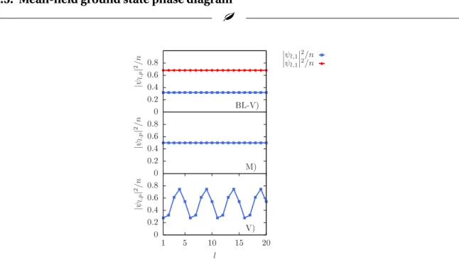
We have verified this prediction by the numerical solution of the DNLSE, and we con-firm that no vortex is found at finite interactions and the density profile is of biased-ladder type, as illustrated in Fig. 2.9 and in the phase diagram (Fig. 2.11, lower panel). By per-forming calculations at varying system size, we find that the imbalance among the two
2.4. Mesoscopic effects and commensurability of the flux f −π 0 π 0 0.5 1 5 10 15 20 θl, 1 / 2 θl,1 θl,2 nl, p / n l −2π −π 0 π 2π 0 0.5 1 5 10 15 20 θl, 1 / 2 θl,1 θl,2 nl, p / n l
Figure 2.8: Phase and density profiles of the condensate wavefunction for non-interacting bosons along the double ring lattice as a function of the lattice index. Top panel: odd number of vortices for average fluxΦ = π/Ns. Bottom panel: even number of vortices for
Φ = 0. The other parameters are K /J = 0.8, φ = π/2,Ns= 20 and n = N /Ns.
rings decreases with increasing Ns.
It is interesting to notice that this is different from the case of the biased ladder phase BL-V obtained for values of flux corresponding to even multiples ofπ/Ns. In this case, the
particle imbalance does not depend on Ns and the phase is also found in the
thermody-namic limit.
2.4.3 Spiral interferograms
It has been shown [67, 68, 69] that it is possible to reconstruct the phase pattern of ring trapped Bose-Einstein condensate by studying its interference pattern with a reference disk-shaped condensate placed at the center of the ring. Using a similar principle, we show here that the interference pattern of two concentric rings allows to characterize the vortices in the bosonic double ring lattice.
Assuming that the distance between neighbouring sites on each ring is larger than the difference of the radii of the two rings, the main contribution to the interference process is due to radially overlapping condensates belonging to the same site index in each ring (ie with the same angular coordinate). In this case, the wave function after after a time tT OF
from releasing the double ring trap is given by (see Appendix D for details):
Ψp(r,θl) ≈ ˜Ψ0(ks,p)ei ħ
k2s,p
2mtT OFeiφl ,ppn
l ,p (2.18)
whereφl ,p and nl ,p are respectively the phase and the number of particles of a
conden-sate on the ring p at site l , and ks,p =
(Rp−r )(−1)pm
0 0.2 0.4 0.6 0.8 1 1 5 10 15 20 U n/J = 0 0 0.2 0.4 0.6 0.8 1 5 10 15 20 U n/J = 0 U n/J = 0.1 |Ψ l, p | 2 / n l |Ψl,1|2/n |Ψl,2|2/n |Ψ l, p | 2 / n l
Figure 2.9: Density profile for a double ring lattice of interacting bosons with total flux Φ = π/Ns, in the absence of interactions, single vortex in the Meissner phase (upper panel)
and for weak repulsive interactions biased-ladder (BL-M) phase (lower panel). The other parameters are Ns= 20,K /J = 2,φ = π/2.
wave function evolve after releasing the trap. The interference pattern intensity is given by I (r,θ) = 2 Re[Ψ∗1(r,θ)Ψ2(r,θ)]. By recalling that in density-phase representation
p
nl ,1nl ,2ei (φl ,1−φl ,2)= 〈a†l ,2al ,1〉, (2.19)
we obtain the following intensity distribution in the polar plane (r,θl):
I (r,θl) = 〈a†l ,1al ,1〉 + 〈a†l ,2al ,2〉 + 2Re
h ei∆ReiQr〈a† l ,1al ,2〉 i (2.20) with Q =m(R1−R2) ħtT OF and∆R= (R2 2−R21)m ħtT OF .
In order to analyze typical interference profiles in the various phases, we start from the non-interacting regime. In this case, using the results of Appendix A, in the Meissner
2.4. Mesoscopic effects and commensurability of the flux f -4-3-2-1 0 1 2 3 4 Qx/(2π) -4 -3 -2 -1 0 1 2 3 4 Q y / (2 π ) -4-3-2-10 1 2 3 4 Qx/(2π) 0 0.01 0.02 0.03 0.04 0.05 0.06 0.07 0.08 -4-3-2-10 1 2 3 4 Qx/(2π) -4 -3 -2 -1 0 1 2 3 4 Q y / (2 π ) -4-3-2-1 0 1 2 3 4 Qx/(2π) 0 0.01 0.02 0.03 0.04 0.05 0.06 0.07 0.08
Figure 2.10: Spiral interferogram in the Meissner phase (upper panels) with K /J = 1.5,
φ = π/2 and Un/J = 0.3 , Φ = 0 (upper left panel), Un/J = 0, Φ =Nπs (upper right panel), and in the vortex phase (lower panels) taking K /J = 0.1,Un/J = 0.3, φ = π/3, with Φ = 0 (lower left panel), andΦ =Nπ
s (lower right panel). In all panels Ns= 35. phase one readily obtains
I (r,θl) ∝
1
Nscos(Qr + ∆
R) + nθl (2.21)
where nθl = 〈a†l ,1al ,1+ a†l ,2al ,2〉. This corresponds to an interference pattern made of
con-centric rings, as illustrated in the first panel of Fig.2.10.
In the case of a single vortex in the Meissner phase, (second panel of Fig.2.10) the in-terference pattern displays a line of dislocations, which are due to the phase slip and van-ishing of the density in correspondence of the vortex core.
In the vortex phase, Eq.(2.20) yields
I (r,θl) ∝ 1 Ns [2uk1vk1cos(Qr + ∆R) + vk2 1cos(θl(k2− k1) − ∆R−Qr ) + u2k 1cos(θl(k2− k1) + ∆R+Qr )] +nθl. (2.22)


![Figure 1.7: a) Ground-state energy of the Lieb-Liniger model versus interaction strength, from [56]](https://thumb-eu.123doks.com/thumbv2/123doknet/14616264.733115/26.918.150.724.106.459/figure-ground-state-energy-liniger-versus-interaction-strength.webp)


![Figure 3.1: The upper panel represents the excitation spectrum of an homogeneous BEC from [85]](https://thumb-eu.123doks.com/thumbv2/123doknet/14616264.733115/53.918.146.799.106.608/figure-upper-panel-represents-excitation-spectrum-homogeneous-bec.webp)


