HAL Id: inria-00327254
https://hal.inria.fr/inria-00327254
Submitted on 7 Oct 2008HAL is a multi-disciplinary open access
archive for the deposit and dissemination of sci-entific research documents, whether they are pub-lished or not. The documents may come from
L’archive ouverte pluridisciplinaire HAL, est destinée au dépôt et à la diffusion de documents scientifiques de niveau recherche, publiés ou non, émanant des établissements d’enseignement et de
Description and simulation of dynamic mobility
networks
Antoine Scherrer, Pierre Borgnat, Eric Fleury, Jean-Loup Guillaume, Céline
Robardet
To cite this version:
Antoine Scherrer, Pierre Borgnat, Eric Fleury, Jean-Loup Guillaume, Céline Robardet. Description and simulation of dynamic mobility networks. Computer Networks, Elsevier, 2008, 52 (15), pp.2842-2858. �10.1016/j.comnet.2008.06.007�. �inria-00327254�
Description and simulation of dynamic
mobility networks
A. Scherrer
a, P. Borgnat
a, E. Fleury
b,∗,
J.-L. Guillaume
cand C. Robardet
daUniversit´e de Lyon, ENS Lyon, Laboratoire de Physique (UMR 5672 CNRS),
69364 Lyon cedex, France
bUniversit´e de Lyon, ENS Lyon, INRIA/ARES, Laboratoire de l’Informatique du
Parall´elisme (UMR 5668), 69364 Lyon cedex, France
cUniversit´e Pierre & Marie Curie, LIP6 (UMR 7606 CNRS), France dUniversit´e de Lyon, INSA-Lyon, LIRIS (UMR 5205 CNRS), France
Abstract
During the last decade, the study of large scale complex networks has attracted a substantial amount of attention and works from several domains: sociology, biology, computer science, epidemiology. Most of such complex networks are inherently dy-namic, with new vertices and links appearing while some old ones disappear. Until recently, the dynamic of these networks was less studied and there is a strong need for dynamic network models in order to sustain protocol performance evaluations and fundamental analyzes in all the research domains listed above.
We propose in this paper a novel framework for the study of dynamic mobility networks. We address the characterization of dynamics by proposing an in-depth description and analysis of two real-world data sets. We show in particular that links creation and deletion processes are independent of other graph properties and that such networks exhibit a large number of possible configurations, from sparse to dense. From those observations, we propose simple yet very accurate models that allow to generate random mobility graphs with similar temporal behavior as the one observed in experimental data.
Key words: Dynamic Networks, Network Models, Complex Systems, Random Graphs, Statistical Analysis, Stochastic Process, Data Mining.
1 Introduction
During the last decade, the study of large scale networks has attracted a large amount of attention and works from several domains: sociology [39], biology [23], computer science [1], epidemiology [33]. Consequently, complex networks have become a new area of research. This emerging domain has proposed a large set of tools that can be used on any complex network in order to get a deep insight on its properties and to compare it to other networks. Such fundamental properties [1,30,31] are used as characterization parameters in the study of various problems such as virus spreading [20,29,33] in the epidemiology context, or information / innovation diffusion [2,21] for instance.
However, a fundamental property of complex networks has been, until re-cently, less studied: the evolution in time, i.e. their dynamical aspect. Indeed most complex networks change, new nodes and edges appear while some other disappear, and in all the scientific domains cited above, the dynamic is an in-trinsic property: people make new acquaintances, change their relations, new machines are added on the Internet, communication links fail, etc. Therefore it appears crucial to better understand the intrinsic characteristics of such dy-namic complex networks, first to get knowledge but also to be able to simulate them. Most studies that address dynamic networks consider growing models, such as the preferential attachment model [26], or analyze the aggregation of all interactions. Both approaches may miss the real dynamic behavior.
In this paper, we address the description and the simulation of sensor mobility networks, in which nodes are human beings and relationships (links) are the ability of a wireless communication to take place. Even though such networks have obvious specificities, the in-depth study of their dynamic is an original work, and can have a broader impact on the complex system community.
A first contribution of this paper is to introduce some simple methods to describe the network dynamics, based mainly on two approaches. First, we study graph properties, such as the number of links or the average degree, as
⋆ This work is partially financed by the European Commission under the Frame-work 6 HealthCare Project LSH PL037941 “Mastering hOSpital Antimicrobial Re-sistance and its spread into the community” (MOSAR) and AEOLUS project IST IP-FP6-015964. The views given herein represent those of the authors and may not necessarily be representative of the views of the project consortium as a whole. ∗ Author for correspondence. ´Ecole normale sup´erieure de Lyon – 46, all´ee d’Italie – 69364 Lyon cedex 07 – France. Fax: (+33) 4 72 72 88 06
Email addresses: [email protected] (A. Scherrer),
[email protected] (P. Borgnat), [email protected] (E. Fleury), [email protected](J.-L. Guillaume),
function of time (possibly in a multivariate way), so as to give an empirical statistical characterization of the dynamics. Second, we compute global indi-cators from the dynamics of the network (stability of connected components, triangles creations, existence of communities) and more specially the activities of the link – indicators that are not simply related to a succession of static snapshots of networks. The proposed methods come from various research do-mains (signal processing, graph theory and data mining). This emphasizes the necessity of interdisciplinary research since dynamic networks are becoming a central point of interest, not only for engineers and computer scientists but also for people in many other fields. We applied those methods on two real-life dynamic mobility networks, based on sensor measurements. The chosen anal-ysis, directly from the data of real dynamical networks, has the interest that it is independent from any modeling of the dynamics, or of individual agents. The second contribution of this paper is to propose simulation models founded on the observations made though our extensive set of analyzes. These models aim at reproducing the major properties of the dynamic mobility network un-der study. By introducing several models, we are able to highlight the diversity of properties that are needed to characterize such networks. Furthermore, our models provide insight into existing notions of dynamic networks and demon-strate that the structure and the dynamics are complex and are not a direct consequence of the contact and inter-contact durations. Proposing such models is crucial since it enables a validation of the ongoing research conducted in the various areas that deal with dynamic networks. It has also many applications in performance evaluation for instance.
The article is organized as follows. In Section 2, we present the data traces we have used in our experiments. In Section 3 we describe and analyze the evolution in time of the network and in Section 4 a global analysis of the dynamics is given. Then, we introduce in Section 5 various random dynamical models adapted to the experimental data sets. Related works are reported in Section 6 and we reach the conclusions in Section 7, stressing that many open problems remain to study, and we present future works related to further improvements of the models as well as in situ data gathering on a larger scale.
2 Data sets
In this paper, we study two mobility networks based on sensor measurements. The Imote [11] data set has been collected during the Infocom 2005 confer-ence. Bluetooth sensors have been distributed to a set of participants who were asked to keep the sensors with them continuously. These sensors were able to detect and record the presence of other Bluetooth devices inside their radio-range neighborhood. The available data concern 41 sensors over a period
of nearly 3 days which represent 254151 seconds. The sampling time (between 2 beacons) is ζ = 120 seconds.
The Mit or Reality Mining [17] experimental data set is constituted of records from Bluetooth contacts for a group of cell-phones distributed to 100 MIT students during 9 months. Each cellular phone completes a Bluetooth device discovery scan and records the identities of all devices present in its neighbor-hood at sampling period of ζ = 300 seconds.
For both data sets, the Bluetooth devices may discover any kind of Bluetooth objects in its neighborhood. We have restricted our analysis to internal con-tacts only. Note also that the sensors had no localization capability, therefore we do not have information on the actual movements of individuals carrying the sensors or on the proximity of two given sensors. The sampling period ζ for probing neighboring nodes defines a minimum resolution time: it means that details at time-scales finer that ζ are not accessible (it is a kind of low-pass filtering of the real dynamical data). Finally we consider that adjacency is a “physical proximity” which is inherently an undirected quantity (the neigh-boring relation is symmetric).
3 Statistical analysis of snapshots of graphs
This section is devoted to the analysis of standard graph (or network) prop-erties (classically used for static networks) as a function of time. For that, we resort to statistical signal processing to uncover the temporal evolution of the sequence of graphs.
3.1 Standard graph properties
Successive snapshots of the network.At a given time step, a snapshot of the interactions that exist in the data set is modeled by a graph Gt= (V0, Et)
with t ∈ N, the time index, constructed as follows: a link {uv} ∈ Et exists if
one finds, in the collected data set, a tuple hu, v, t1, t2i for which t ∈ [t1, t2].
Here, the set of vertices V0 does not change in time as we are interested in the dynamical aspect of the interactions, rather than in the network growth (see for instance [26]). The sampling period of the series Gt will be taken as
1s for all analysis. Note that, because ζ > 1s, we are sure that this sampling step will ensure a well-resolved, slowly changing dynamics for Gt. For each
link e in E0 (the set of all possible edges), we define its state evolution S
e(t)
with Se(t) = 1 if e ∈ Et, 0 otherwise. Looking at the time evolution of Gt
Some standard properties in graph theory are recalled. Nodes are said adja-cent (or neighbors) if there is a link connecting them, and connected if there is a path from one to another (a sequence of adjacent vertices linking both vertices). We note NG(u) the set of neighbors of vertex u and its cardinal is
the degree of u: dG(u) = |NG(u)|. A vertex is connected if its degree is at least
one. The number of links in the graph is noted E(t) = |Et|; the number of
connected vertices is V (t) = |{u ∈ V0, d
Gt(u) > 0}|; and the average degree
of connected vertices is D(t) = P
u∈V0dGt(u)/V (t). Among the more
elabo-rated graph properties, important ones are those related to the identification of “communities” which are loosely defined as collections of individuals who interact with unusually high frequency. For that, we need to quantify the con-nectivity of the vertices, using the following measurements. The set of triangles in a graph, referred to as TG, is the number of subgraph that are triangles,
i.e. subgraphs of 3 vertices all connected one with another. T (t) = |TGt| is
the number of triangles in the graph. This is an important feature to charac-terize how frequently trio of people exists. A connected component (CC) is a maximal subgraph such as every node of the subgraph is connected to each another node; CG(t) is the set of connected components (excluding isolated
nodes) and Nc(t) = |CGt| is the number of such CC.
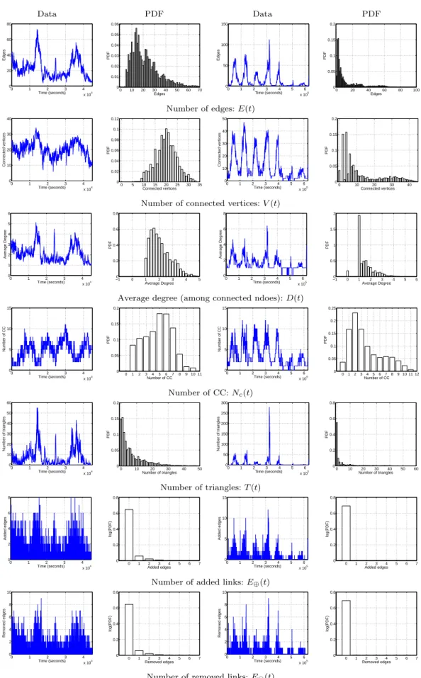
Typical characteristics. For each time series, the probability distribution function (frequency of observation) is estimated over the duration of the obser-vation, using empirical histograms of the data. The mean of the distributions is then computed, together with the standard deviation (average of the square deviations from the mean) in order to give an idea of their variability. Results for a typical day of the Imote data set, and a typical week of the Mit data are reported in Fig. 1 and in Tab. 1. We have carefully checked that the re-sults obtained on these durations were similar for other periods. Both Imote and Mit graphs are sparse (the number of links is low): the proportion of ac-tive links is always less than 10% for the Imote data, among the 820 possible links, and is even lower in the Mit data with less than 2% of the 4950 possible links. During daytime, all properties exhibit large variations, yet one can note that at no time the network is a single connected component. Many nodes remain isolated during long times (around 50% on average for daytime and more than 90% for nighttime). Conversely, the number of triangles is rather large when compared to random graphs with the same density. For an Erd¨os-R´enyi random graph [18] with N vertices (each link appears independently with probability p), the expected number of triangles is ³N3´3!p3 for low
den-sity graphs [6]. The expected number of links is pN (N − 1)/2, so when there are k links in the graph, the expected number of triangles is ∼ N8k23(N −1)(N −2)2. If the
Imotedata was modeled by a random graph, from the maximum number of links (70), one would expect a maximum number of 40 triangles, and from the average number of links (22), one would expect an average number of triangles around 1. Yet one finds respectively 60 and 7. The reason is that if two people
Imote Mit
Property Mean Std. Dev. Corr.
Time (s)
Mean Std. Dev. Corr.
Time (s)
#Active links E(t) 21.9 12.4 5200 13 17.7 16800
#Connected vertices V (t) 19.9 4.7 7400 12.3 11.6 17500 Avg degree D(t) 2.1 0.8 3600 1.5 0.8 7300 #CC Nc(t) 4.8 2.1 5600 3.7 2.7 5200 # Triangles T (t) 6.9 8.30 4700 6.6 19.8 5500 Edge creation E⊕(t) 0.15 0.55 680 0.005 0.11 30 Edge delation Eª(t) 0.15 0.55 680 0.004 0.08 260 Table 1
Graph properties: Mean and Standard Deviation of PDF, Correlation Times.
can communicate with a third one, it is likely that they can also communicate with each other, all three people being near each other. However, this property is here uncovered from empirical statistical analysis, without any assumption on the real-world topology or on the behavior of people.
Probability distribution. The empirical histograms, computed on a time-bin of 1s (much smaller than the protime-bing time, so that the specific choice of this bin-size has no effect) are displayed in Fig. 1. The various estimated probability distributions obtained are not heavy tailed, meaning that the variability is not very large and the standard deviation is a good measurement of the variability.
3.2 Dynamical characteristics
Correlation times.For all the properties of Gt discussed so far (E(t), V (t),
D(t), Nc(t) and T (t)), the temporal evolution is characterized first as
univari-ate time-series. The autocorrelation function for a quantity X(t) is estimunivari-ated empirically as: CX(τ ) =< X(t + τ )X(t) >t − (< X(t) >t)2, where < · >t is
the mean over time (this results in the well-known biased estimator for the stationary autocorrelation [32]). The correlation time is then defined as the first time where the function CX(τ ) goes to zero (this always happens due to
the summation rule of empirical CX). It quantifies the “memory” of the series:
the longer it is, the greater is the persistence of fluctuations in the data.
An important note is that the series do not look stationary, especially if seen at a large time-scale, e.g. there are clear periods of one day and variations from days to nights. At night, the numbers of vertices and links change less, and the network is basically a set of disjoint sets of vertices with links certainly corresponding to roommates. Some peaks (up or down depending of the prop-erty under concern) are easily identified in the Imote data, corresponding to lunch (around time t ≃ 1.5 · 104 seconds), afternoon break (t ≃ 2.4 · 104 s) and dinner (t ≃ 3.5 · 104 s). To rule-out the effect of non-stationarity, we first
Data PDF Data PDF 0 1 2 3 4 x 10⁴ 0 20 40 60 80 Time (seconds) Edges 0 10 20 30 40 50 60 70 0 0.01 0.02 0.03 0.04 0.05 0.06 PDF Edges 0 1 2 3 4 5 6 x 10⁵ 0 50 100 150 Time (seconds) Edges 0 20 40 60 80 100 0 0.05 0.1 0.15 0.2 PDF Edges
Number of edges: E(t)
0 1 2 3 4 x 10⁴ 0 10 20 30 40 Time (seconds) Connected vertices 0 5 10 15 20 25 30 35 0 0.02 0.04 0.06 0.08 0.1 0.12 PDF Connected vertices 0 1 2 3 4 5 6 x 10⁵ 0 10 20 30 40 50 Time (seconds) Connected vertices 0 10 20 30 40 0 0.05 0.1 0.15 0.2 PDF Connected vertices
Number of connected vertices: V (t)
0 1 2 3 4 x 10⁴ 0 1 2 3 4 5 6 Time (seconds) Average Degree −10 0 1 2 3 4 5 0.2 0.4 0.6 0.8 PDF Average Degree 0 1 2 3 4 5 6 x 10⁵ 0 2 4 6 8 Time (seconds) Average Degree −1 0 1 2 3 4 5 6 0 0.5 1 1.5 2 PDF Average Degree
Average degree (among connected ndoes): D(t)
0 1 2 3 4 x 10⁴ 0 5 10 15 Time (seconds) Number of CC 0 1 2 3 4 5 6 7 8 9 10 11 0 0.05 0.1 0.15 0.2 PDF Number of CC 0 1 2 3 4 5 6 x 10⁵ 0 5 10 15 Time (seconds) Number of CC 0 1 23 4 5 67 8 9 10 11 12 0 0.05 0.1 0.15 0.2 0.25 PDF Number of CC Number of CC: Nc(t) 0 1 2 3 4 x 10⁴ 0 10 20 30 40 50 60 Time (seconds) Number of triangles 0 10 20 30 40 50 0 0.05 0.1 0.15 0.2 PDF Number of triangles 0 1 2 3 4 5 6 x 10⁵ 0 50 100 150 200 250 300 Time (seconds) Number of triangles 0 10 20 30 40 50 60 0 0.2 0.4 0.6 0.8 PDF Number of triangles Number of triangles: T (t) 0 1 2 3 4 x 10⁴ 0 2 4 6 8 Time (seconds) Added edges 0 1 2 3 4 5 6 7 0 0.2 0.4 0.6 0.8 log(PDF) Added edges 0 1 2 3 4 5 6 x 10⁵ 0 5 10 15 Time (seconds) Added edges 0 1 2 3 4 5 6 7 0 0.2 0.4 0.6 0.8 log(PDF) Added edges
Number of added links: E⊕(t)
0 1 2 3 4 x 10⁴ 0 2 4 6 8 10 Time (seconds) Removed edges 0 1 2 3 4 5 6 7 0 0.2 0.4 0.6 0.8 log(PDF) Removed edges 0 1 2 3 4 5 6 x 10⁵ 0 2 4 6 8 10 Time (seconds) Removed edges 0 1 2 3 4 5 6 7 0 0.2 0.4 0.6 0.8 log(PDF) Removed edges
Number of removed links: Eª(t)
Fig. 1. Statistics of graph properties, displayed as a function of time (Imote on the left and Mit on the right).
remove the slow non-stationary trend on the scale of the day. This is done by estimating the trend by a moving average smoothing of period 104s. It was
checked that the reported results on autocorrelation and the correlation-times are consistent for both the detrended series and the original time-series. The analysis reported here is simple, yet robust. A full non-stationary treatment of the mobility networks is out of scope here, and will be discussed in the perspectives, see Section 7.
The different autocorrelation functions (not shown) for the data (detrended or not) reveal an exponential-like decay. The correlation times of E, V and Nc are rather large and all of the same magnitude: ∼ 1h15 for Imote and
∼ 7h for Mit. The properties D and T have comparable correlation times. This suggests that these properties evolve under a common cause. This will be further investigated in Section 3.3. Even if this characterization of evolution is just a quick overview, the conclusion is that the graph snapshots display many characteristics with similar and correlated behaviors over a long time. The purpose of Section 5 will be to propose a global model for dynamics of network, using the properties found here.
Contact and inter-contact durations. The contact and inter-contact du-ration distributions are dynamic characteristics interesting for mobility net-works. The contact duration is the time during which two vertices remain directly and continuously adjacent. The inter-contact duration is the duration between two periods of contact for two vertices. As observed in [11] for the Imote data, both distributions have a tail that can be modeled by a power law, so that the complementary cumulative distribution functions (CCDF) of contact or inter-contact durations X (seen as a random variable) follows: P [X > x] ∼
x→∞ cx
−α. For α > 2, the associated r.v. X has a finite mean
and a finite variance. For α < 2, X has an infinite variance and is said heavy tailed. Moreover, if α < 1, X has both an infinite mean and an infinite vari-ance. When the variance is infinite, the tail dominates the behavior of the variable, especially it causes large events much more frequently than for non-heavy tailed distributions. Therefore high variability in the data is sometimes explained by heavy tails, as opposed to lower variability which appears for instance with exponentially decaying tails.
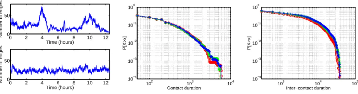
Fig. 2 shows the CCDF of contact and inter-contact durations and the fitted power-law distributions (mean and estimated α are reported in captions), re-spectively for the Imote and Mit data sets. The fits show relevancy of the power-law behavior for both contact and inter-contact duration distributions over a wide range of scales. As already discussed in [11] for the Imote data, the heavy-tailed nature of these distributions seems to be an ubiquitous property of dynamic mobility networks. For both data sets, inter-contact duration dis-tributions have an α lower than 1, meaning very strong variability due to long periods of lack of contact for some vertices, whereas the distribution of contact
Imote 101 102 103 104 105 10−5 10−4 10−3 10−2 10−1 100 Contact Duration P[X>x] 101 102 103 104 105 106 10−5 10−4 10−3 10−2 10−1 100 Inter−contact Duration P[X>x] Mean : 140 - α = 1.66 Mean : 3680 - α = 0.60 Mit 101 102 103 104 105 106 10−5 10−4 10−3 10−2 10−1 100 Contact Duration P[X>x] 102 104 106 108 10−3 10−2 10−1 100 Inter−contact Duration P[X>x] Mean : 3270 - α = 2.4 Mean : 148700 - α = 0.49
Fig. 2. Contact (left) and Inter-contact (right) duration distributions (CCDF).
durations is less heavy-tailed (for Mit it is actually not heavy-tailed at all, with α = 2.4). Accurately modeling such experimental data with power-laws is a complex problem [27], and tackling this issue is beyond the scope of our work. Here the important fact is that those non-trivial empirical distributions should be taken into account when constructing a model.
Dynamics of links creation and deletion. The processes of creation and deletion of links are E⊕(t) = |{e ∈ Et, e /∈ Et−1}|, the number of links added at
time t and Eª(t) = |{e ∈ Et−1, e /∈ Et}|, the number of links removed at time t.
Their temporal evolution and empirical probability distributions are reported in Fig. 1 and mean, standard deviation and correlation time are included in Tab. 1. The distributions here are really narrow. Especially, there are many time-steps with no event. Note that we plot the logarithm of the probability distribution function in order to get rid of such effects, but still they decrease very quickly. Yet, there exists some form of non-stationarity here, with some intermittent peaks of activities, in conjunction with the peaks of the classical characteristics discussed above.
However, the correlation time of the link creation and deletion properties is really much smaller (∼ 13 min. for Imote and ∼ 10 min. for Mit) than the correlation time of all other characteristics. Therefore, these properties can almost be considered memory-less. This is a key property that supports a
E(t) V (t) Nc(t) D(t) T (t) E⊕(t) Eª(t) E(t) 1 0.85 -0.56 0.95 0.90 0.19 0.15 V (t) 0.85 1 -0.20 0.70 0.66 0.15 0.11 Nc(t) -0.56 -0.20 1 -0.70 -0.41 -0.16 -0.15 D(t) 0.95 0.69 -0.69 1 0.86 0.19 0.15 T (t) 0.90 0.66 -0.41 0.86 1 0.15 0.11 E⊕(t) 0.19 0.15 -0.16 0.20 0.15 1 0.03 Eª(t) 0.15 0.11 -0.15 0.16 0.10 0.03 1 Table 2
Imote: correlation coefficients between the various graph properties.
simulation built on a kind of Markovian evolution of the process of creation or deletion of links (see Section 5).
3.3 Multivariate statistics of graph properties
In the following, we describe all the properties as elements of a random vector, and thus explore multivariate statistics.
Cross-correlations.The cross-correlation matrix is computed as the correla-tion coefficient (in time) of each pair of properties. It is presented in Tab. 2 for Imote data (results on Mit are similar). Most of the correlation coefficients are rather high. This is not surprising for two main reasons. First, there are constraints on the properties of graphs. For instance the number of links E(t) has a strong influence on the number of connected vertices V (t); similarly the number of connected component (Nc(t)) is highly related to the number of
links in the graph. Second, we have already noticed that all the peaks seem to happen in the same period of times. They are responsible for a large part of the correlations. Note that some couples of properties are less correlated (number of connected components Nc(t) and number of connected vertices
V (t) for Imote, as well as number of connected components and triangles for both data sets). On the contrary, link creation and deletion processes (E⊕(t)
and Eª(t)) remain mostly uncorrelated with all other properties (correlation
coefficients are always below 0.2), even though they also exhibit an increase of variability during the peak activity periods. Consequently, the link creation and deletion processes can be considered mostly independent from the evolu-tions of other graph properties. This provides a second argument in favor of a simple Markovian (memory-less) link creation/removal process.
Joint distributions.The empirical joint distribution of some couple of prop-erties gives a finer description of the dependencies between those propprop-erties. The joint distribution PXY of two discrete random variables X and Y is
de-fined as: PXY(x, y) = P [X = x and Y = y] = P [X = x/Y = y]P [X = x].
Imote 0 10 20 30 40 0 20 40 60 80
Number of connected vertices
Number of edges 0 10 20 30 40 0 10 20 30 40 50 60 70 80 Number of vertice Number of edges Mit 0 10 20 30 40 50 0 20 40 60 80 100 120
Number of connected vertices
Number of edges 0 10 20 30 40 50 0 20 40 60 80 100 Number of vertice Number of edges
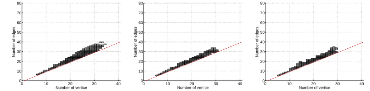
Fig. 3. Imote: Stationary joint distribution of the number of connected vertices V (t) and the number of links E(t) (left), and joint distribution per individual connected component of the number of links and vertices (right), for Imote and Mit data sets. The gray scale is proportional to the logarithm of the probability (black means higher probability, and white no occurrence of this event in the data).
data sets), globally (left) and inside CCs (right).
As expected, the plots exhibit a positive correlation between vertices and links. The more vertices are connected, the more links are present, since the mini-mum number of links is half the number of connected vertices (if the network is a set of disjoint links) and the maximal number is V (t)(V (t)−1)/2. However it is worth noting that the variation of the number of links is not constant over the number of vertices1 with a variation which is approximatively quadratic
in the number of vertices. This means that, for a given number of vertices, the network can have a large number of possible configurations, some of which are very sparse and others more dense, as shown by the gray scale in the plots. Fig. 3 (right) shows the same joint distribution inside connected components. One can also observe a positive correlation between the number of vertices and links in a connected component with a non-constant variation of the number of links. For Imote data, the variation factor is around 4.5 which means that for a given number of vertices, one can expect a variation of density of the same order of magnitude. These joint distributions have a significantly differ-ent shape for simple random dynamic graph model. This will be discussed in Section 5 (see also [19]).
−0.40 −0.2 0 0.2 0.4 0.6 0.8 1 2 4 6 8 10 12x 10 4 Correlation coeficient
Number of edge couples
−0.50 0 0.5 1 1.5 2 4 6 8 10 12 14x 10 4 Correlation coeficient
Number of edge couples
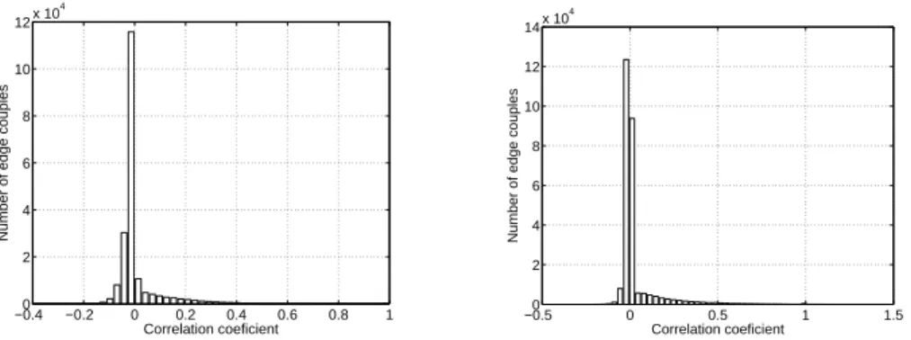
Fig. 4. link correlation histogram for Imote (left) and Mit (right).
Links correlations.The correlation coefficient of the state evolution of links Se(t) characterizes the dependency between links. Here the links that are never
active are discarded. Indeed, in the first day of the Imote data set, more than half of the links never appear. Fig. 4 shows the histogram of the values for both data sets. Most pairs of links have a very low correlation coefficient. It is therefore reasonable to consider that links are independent, even if some rare couples of links exhibit a strong correlation: 0.23% of couples in Imote (0.04% in Mit) have a correlation coefficient larger than 0.5.
4 Towards a global analysis of the dynamics
We now turn to global properties that are not directly interpretable in the sequence of static graphs in order to characterize the dynamics of a graph as a whole. We study hereafter the stability of connected components (and hence of the information paths between vertices), the proportion of creation of triangles observed as well as the communities embedded in the network.
4.1 Stability of Connected Components
As defined in section 3.1, a connected component (CC) is a maximal subgraph such that a path exists between every pair of vertices. The set of links is im-portant and two similar sets of vertices with different set of links are assumed to be different components. However, a set of connected vertices is a set of vertices that can communicate, therefore the identification of such sets is also interesting from a networking point of view. We denote such sets as CCN. Previous results (see Fig. 1) show that most of the time there are many CCs and that there is nearly no time step during which there is only one CC. To go deeper in the study of these subgraphs, we have computed all the CCs and CCNs which existed during at least one time step in order to study their
stability. During the first day of Imote (resp. Mit), we have obtained 6819 CCs and 2608 CCNs (resp. 2728 and 1272), among which 292 (resp. 250) are isolated links. This means that, on average, less than 3 different configurations of links (CCs) are built over a given set of vertices (CCNs) for both data sets. In the following we will only display plots for Imote since the results for Mit are very similar. Results will be discussed for both data sets.
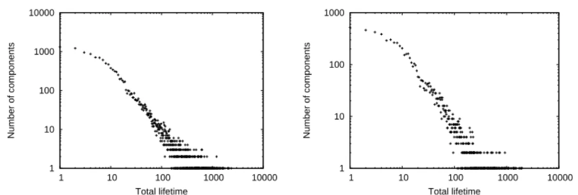
1 10 100 1000 10000 1 10 100 1000 10000 100000 Number of components Total lifetime 1 10 100 1000 10000 1 10 100 Number of components Number of appearances
Fig. 5. Distribution of the total lifetime (left, a), number of appearances (right, b) for all CCs (+) and CCNs (x) of Imote.
In the following, the total lifetime of a CC c is defined as the number of time steps for which c exists, and the number of appearances of c is the number of time steps t for which this CC is absent at t and present at t + 1. Fig. 5(a) and 5(b) display the distributions of the total lifetime and the number of appearances of all CCs and CCNs for Imote. These plots exhibit a strong heterogeneity for both parameters. While more than 52% of the CCs and 40% of the CCNs exist only during one time step for Imote, some of them exist during a quarter to a third of the whole time. The plots are very similar for Mit but due to the measurement method there is nearly no CCs and CCNs with a very short lifetime, but some last for more than half of the total duration. The most frequent CCs and CCNs are just couples of vertices for both data sets.
1 10 100 1000 10000 100000 0 5 10 15 20 25 30 35 Total lifetime Number of nodes 0 5 10 15 20 25 30 0 5 10 15 20 25 30 35 Number of appearances Number of nodes
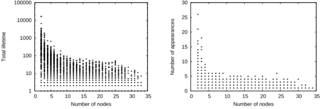
Fig. 6. Joint distribution of the number of vertices and total lifetime (left, a), and joint distribution of the number of vertices and number of appearances (right, b) for all CCs of Imote.
distribu-tion of the number of vertices and total lifetime for all CCs of Imote. The absence of stability of large CCs is striking: there is no CC with more than 8 nodes (while 67% CCs have more than 8 nodes) which have a lifetime greater than 100 seconds. Similar results are obtained for CCNs: there are 36 of such sets (among 47% of all CCNs), and the oldest is of size 10 and lives for 262 seconds. The more links and vertices a CC or a CCN contains the more poten-tial modifications may happen, which explains in part the curves. However, we could have expected that such sets would be stable for longer periods. Fig. 6(b) presents similar results for the joint distributions of the number of vertices and number of appearances for all CCs of Imote. Again the CCs which reappear regularly are only small components. The plots might lead us to believe that some large CCs appear regularly more than once. However, if we admit that a component reappears only if it has disappeared for more than five minutes, then no CCs of size greater than 6 appear more than once (representing 73% of all CCs). For CCNs the same condition yields only 12 components, none of them appearing more than twice2. This means that most CCs and CCNs
reappear very soon after they have disappeared, which is a direct consequence of links and vertices flickering: if a link is added then removed, the correspond-ing CC ceases to exist then reappears. If a vertex leaves a CCN and comes back later on the same applies for the corresponding CCN. Again we do not detail results for Mit, which are very similar to the ones for Imote.
+0 +1 +2 +3 +4 -0 41146 382 1 1 -1 384 6599 615 32 3 -2 632 114 31 -3 29 25 2 2 -4 1 1 +0 +1 +2 +3 +4 -0 352 1 -1 351 2461 168 6 -2 175 11 1 -3 3 -4 Table 3
Number of evolution of each type for Imote (left, a) and Mit (right, b): a (+x, −y) = k cell meaning that there is k time steps where x CCs appear and y CCs disappear simultaneously.
Finally, Table 3 gives the number of time steps for which specific events hap-pen. For Imote, among the time steps where at least one CC appears or disappears, 74% correspond to one CC appearing for one disappearing. This certainly means a link or a vertex modification. However, the other 26% are time steps during which we can see CCs appearing from scratch, disappearing completely, or even merging/splitting. For Mit the results are very similar, but there are fewer events that concern many components.
The dynamical effects observed at a global scale are also present in large CCs and CCNs. They have a very short lifespan and one can not expect that they
2 A CCN of size 30 appears twice with an interval larger than 5 minutes with a
would reappear in the future. On the contrary, small CCs are generally more stable and have a much higher probability of reappearance.
4.2 Triangles in the graphs
The existence and persistence of connected components is generally associated with a rather large number of triangles in the graph. Therefore, it is interesting to ask: what is the proportion of links that create triangles when they appear? To answer this question we have to evaluate the number of link creations that leads to an increase of (resp. does not change) the number of triangles in the graph. Let P+/tri+ (resp. P+/tri=) be the proportion of link creations
that increase (resp. does not change) the number of triangles in graph. Let further f+/tri+ (resp. f+/tri=) be the average proportion of inactive links that
would create a triangle if activated. These proportions are given in Table 4 (in percentage) for Imote data, Mit data and for a simple random dynamical graph (with independent contact and inter-contact distribution distributed as a power-law; this will be further described in Section 5). One can see that for both data sets, around 40% of link creations increase the number of triangles in the graph, which is a fairly large proportion when compared to a simple random dynamical graph (∼ 10%). The proportion of inactive links that would create a triangle is very low for both experimental data sets and the simple random graph. This emphasizes the fact that this is not because more links can create triangles that the proportion P+/tri+is higher in experimental data:
it is on the contrary a intrinsic property of the dynamics. This property will actually be used in random dynamic graph models in Section 5.
P+/tri+ P+/tri= f+/tri+ f+/tri=
Imote 44 % 56 % 6 % 94 %
Mit 40 % 60 % 7 % 93 %
Random 10 % 90 % 5 % 95 %
Table 4
Proportion of link creations that adds a new triangle or not (P ), and proportion of inactive links that, if created, would add a triangle, or not (f ).
4.3 Communities in dynamic interaction networks
Intrinsic structure of a dynamic mobility network is studied by isolating “com-munities”, which are commonly considered as large groups of individuals who interact intensively with each other over a (not necessarily continuous) long period of time. In other words, a community can be seen as a dense connected subgraph that appears in a large number of time steps. The difference with CC and CCN is that communities may have existence spread in non-adjacent
periods of times. In existing approaches [13,14,36], communities are first iden-tified in some time windows and then combined to capture their dynamics. As the problem is NP-hard, those solutions are based on heuristics that ap-proximate the optimal solution. On the contrary, our approach is based on an exact enumeration process, using pruning techniques to practically solve NP-hard problem by means of tight constraints that reduce significantly the search space.
Unfortunately, such dense connected subgraphs cannot be directly computed using the pattern mining under constraints framework (see [28]), since the density has no monotonic properties with respect to an enumeration order of subgraphs. Therefore no pruning technique is available to reduce the search space consisting of all possible subgraphs. To get rid of this difficulty we pro-pose a two-step procedure. First, we gather information on groups of links over time by computing large connected subgraphs that appear at least τ times in the data. We then filter the obtained subgraphs to retain the densest ones. In the second step, we go back to individuals that are present in the result-ing subgraphs. We merge the subgraphs that concern similar individuals and time steps to obtain important and established subgraphs. This enables us to take into account the time variability of the information gathered experimen-tally. Finally, we build the dynamic trajectories of individuals by considering for each individual the community he/she belongs to and we sort them with respect to time to obtain the trajectories.
The two steps are described hereafter. A subgraph S of Gt is denoted by
S ⊆ Gt in the following. We compute the set of connected subgraphs having
more than σ links and that are included in at least τ graphs: C = {S = (V, E), |{t | S ⊆ Gt}| ≥ τ and |E| ≥ σ and S is connected}.
The above three constraints are monotonic if candidate subgraphs and time steps are enumerated all together. This monotonicity allows us to use D-miner [5], a data mining algorithm dedicated to this kind of enumeration processes. Next, among these subgraphs, we select the ones that are sufficiently dense with respect to a parameter δ: Cδ =
n
S ∈ C | |V |(|V |−1)2 |E| ≥ δo.
The second step consists in merging the connected subgraphs that are similar by their set of vertices and their temporal support. Considering two subgraphs S1 = (V1, E1) and S2 = (V2, E2) having respectively temporal supports T1 and
T2. They are merged with respect to ∆ if V1 ⊆ V2, and ∀t ∈ T1 \ T2, ∃t0 ∈
T2, |t − t0| < ∆. Finally, subgraphs S = (V2, E1 ∪ E2) associated with time
step set T1∪ T2 are considered as communities.
Results obtained on the Imote and Mit data sets are reported in Tab. 5 (with the parameters used as well as basic subgraph properties obtained in the first step of the procedure). In order to keep a fewer number of subgraphs, we
τ σ Number Avg. node num. Avg. edge num. Avg. time steps
Imote 7 6 27507 7.9 8.3 8.2
Mit 10 14 30144 10.5 12.8 18.1
Table 5
Algorithm parameters and frequent connected subgraphs properties.
first select the connected subgraphs that have a density greater than δ = 0.8. This gives us 138 dense connected subgraphs for Imote and 1226 for Mit. Note that these dense connected subgraphs cover the same sets of vertices for similar time steps many times. In other words, some of these groups are similar to each other in that they differ by only few individuals or few time steps. Then, we apply the merging procedure using ∆ = 15 (30 min. in real time) to obtain communities, i.e. distinct dense connected subgraphs and their associated time step sets. The result is that Imote data set is structured by 14 communities (see Fig. 7), whereas there are 9 communities on the Mit data set.
From these communities we derive the trajectories of the individuals. The trajectory of each individual in the communities of Imote data is displayed in Fig. 7. Boxes represent individuals entering a group and links are labeled by the individual number when he/she goes from one group to another. The graph is oriented: an arc (u,v) represents individuals moving at least once in the data from group u to group v. For example, individual 8 initially belongs to group 13, he/she further moves into group 6, and finally enters group 7. Results on Mit are similar and are not reported here. Note that these techniques use exhaustive methods and algorithms but still require a supervisor to fix several thresholds and parameters to drive the graph structural exploration.
Let us emphasize then as a conclusion to this global analysis, that the dynamic mobility networks studied disply non-trivial properties: existence of communi-ties, importance of triangle dynamics and stability of connected components. These properties are to be central ones to keep in modeling those networks.
5 Modeling of the dynamics
From the observations detailed in Sections 3 and 4, we propose generic random dynamic models that allows to generate random dynamic graphs which have a behavior similar to the one observed in experimental data sets.
i1 g0 g2 36 i2 g4 g5 2, 14, 24 i4 g3 g1 4, 11, 32 g10 4, 11, 32 i5 i6 g8 14, 24 g12 6 i7 i8 g13 40 g9 19 g6 8 i9 i10 i11 39 11 i13 g7 32 13 i14 i15 i16 g11 32, 35, 38 i17 4, 11, 32 4, 11, 32 i19 i24 i25 i26 i27 i28 4, 11, 32 i30 i32 8 32, 35, 38 i34 i35 i36 i38 i39 i40 35 32 32, 35, 38
Fig. 7. Individual trajectories in groups ordered by time. ix (boxes) are individuals
while gx (circles) denotes social groups.
5.1 Simulation algorithm
The simulation is based on a transition model with Markovian property. For each time step and for each link independently, each link e will change its state (active or inactive) with transition probability Ptr(e, Gt). The corresponding
algorithm is displayed as Algorithm 1. The transition probability depends only on the state of the network, in particular on the duration τ (e) since the link e has last changed its status (up-time if the link is active, down-time if it is inactive). The assumptions that the transition probabilities are independent from one time step to another hold because the processes of link deletion or suppression were found to have a correlation time much smaller than any other property of the graph. Moreover, we can consider each link indepen-dently since link correlation coefficients were found very low. Several models for the transition probabilities are proposed hereafter, first using only the contact and inter-contact duration distributions, second incorporating more elaborated graph properties (global distributions or links behavior), and finally incorporating dynamical information by means of the dynamical behavior of triangle creation process.
Contact and inter-contact duration distributions. A basic point of the dynamics was expressed as heavy-tailed distributions for contact and inter-contact durations (referred to as PON and POF F respectively), as discussed in
Section 3.2. Supposing them to be stationary distributions for the system, we derive the transition probabilities of the link, depending on τ (e) (time since the link is in the state). Let P+(τ ) be the probability that one link that was
Input: Simulation time
Output: Random Dynamic Graph foreach Simulation Time Step t do
foreach link e do
Ptr(e, Gt) = TransitionProbability(e) given the state Gt
pr = Uniform(0,1) if (pr ≤ Ptr(e)) then ChangeState(e) end end end
Algorithm 1.Simulation algorithm
OFF (i.e., inactive) since τ (τ ≥ 1) is activated (going from OFF to ON), at a given time. Similarly, let P−(τ ) be the probability that one link that was
ON (i.e., active) for a time τ (τ ≥ 1) is deleted (going from ON to OFF). The probability that a contact will last for τ time steps can be computed as the probability that the link disappeared after τ multiplied by the probability that the link did not disappear in the preceding τ − 1 time steps. It can be expressed as PON(τ ) = P−(τ ) × Qτ −1i=1(1 − P−(i)). One can then invert this
relation and compute P−(τ ) (resp. P+(τ )) recursively as:
P−(τ ) = PON(τ ) Qτ −1 i=1(1 − P−(i)) , τ ≥ 2, P−(1) = PON(1) (1) P+(τ ) = POF F(t) Qτ −1 i=1(1 − P+(i)) , τ ≥ 2, P+(1) = POF F(1) (2)
It is easy to check that all resulting sequences of graphs Gtwill share on average
the prescribed distribution of contact and inter-contact durations. As we will show later on, these transition probabilities are not sufficient to reproduce the evolution of classical graph properties discussed beforehand. It is then worth introducing other elements in the transition probability.
Models with imposed graph property distribution. To explore the rel-evance of properties such as E(t), V (t), NC(t) and D(t), the probability of
transition is weighted by a probability of acceptance of the new state de-pending of the experimental distribution for a property of interest. This is implemented by Rejection Sampling [35], based on a Metropolis-Hastings al-gorithm [22]. The new proposed state, denoted G′
t = {Gt+ Se(t) changed},
is accepted with probability PRS(Gt, G′t) = min ³
1,F (x(G′t))
F (x(Gt))
´
if F is the tar-get PDF for the graph. The total probability of transition of link e is then: Ptr(e, Gt) = P−/+(τ (e)) · PRS(Gt, G′t). The rationale of this procedure is to
impose the averaged distributions on the simulated sequence of graphs. This can obviously be extended to any other time-evolving property.
0 2 4 6 8 10 12 0 50 Time (hours) Number of edges 0 2 4 6 8 10 12 0 50 Time (hours) Number of edges 102 103 104 10−4 10−3 10−2 10−1 100 Contact duration P[X>x] 103 104 105 10−4 10−3 10−2 10−1 100 Inter−contact duration P[X>x]
−− Imote / o Model A / ∗ Model B / + Model C
Fig. 8. Number of links for Imote data and model A (left), contact (middle) and Inter-contact (right) duration distributions (CCDF) for classical models and Imote.
Models with imposed dynamics of triangles. The average proportion of links creations that yield triangles is larger than for random graphs as discovered in Section 4.2. Therefore, to take this into account in the sim-ulations, a weight is applied on the transition probability to reproduce the correct dynamical transition process concerning triangles (and not merely the stationary distribution of the number of triangles). Obviously, we do not want to change the mean probabilities of transition. Hence, the weights are chosen such that the mean probability (over all the inactive links) is still P+(τ ).
Us-ing the same notations of Section 4.2, the transition probabilities are corrected with the ratios P+/tri+/f+/tri+ for activation of links that add a triangle, and
P+/tri=/f+/tri= for those that do not. This complies naturally with the fact
that the averaged probabilities of creation are not changed. Nevertheless, it will give a higher transition probability to triangle-affecting transitions, like in Imote and Mit data sets. The weighted probabilities are then:
Ptr(e, Gt) = P+(τ (e)) P+/tri=
f+/tri= for link creation without new triangle,
P+(τ (e))
P+/tri+
f+/tri+
for link creation with a new triangle.
5.2 Set of investigated models
A variety of models using parts of the three ingredients are studied. Note that is was already shown in [19] that merely forcing the contact and inter-contact duration distributions is not sufficient to fully uncover the dynamics of an experimental data set. From all the possible graph properties that can be simulated by our random dynamical graph generator, mainly two graph properties are emphasized for the sake of the clarity: the number of connected components and the number of connected vertices. Because other properties were found highly correlated with one another, the behavior of the simula-tion models is similar with respect to them. The three following choices for imposing probability transitions are discussed:
• A: imposed empirical contact and inter-contact duration distribution only. • B: imposed distributions of contact / inter-contact durations , and of number
of connected components.
• C: distributions imposed contact / inter-contact durations and of number of connected vertices.
Those three settings, referred to as classical, are compared with the same models when adding imposed dynamics of triangles, respectively denoted Aω,
Bω and Cω and referred to as weighted. All models are stationary in that the
parameters are fixed for the full simulation. The simulations presented here are designed to reproduce the first day of conference in the Imote data set (this period corresponds to 0.55 · 105s to 1.0 · 105s), a period where the data
appears conveniently stationary – even though the whole data set is not.
5.3 Simulations results
Classical models. Fig. 8 (left) shows the number of links for first model A and the Imote data. Obviously, as we are considering stationary models, they cannot account for peaks corresponding to lunches, breaks, etc. Simply the av-erage number of links in both Imote and the models is the same. Fig. 8 (right) shows the contact and inter-contact duration distributions of both the original Imotedata and the three classical models. The distributions are almost per-fectly adjusted in all cases, showing that even when targeting a distribution using the rejection sampling step described in Section 5.1, the contact and inter-contact distributions are properly reproduced. This constitutes a basic validation of our simulation procedure.
The distributions of E(t), V (t) and Nc(t) are plotted in Fig. 9. A first
re-mark is that the sole contact and inter-contact duration distributions (model A) dramatically fail to reproduce the properties. More precisely, the num-ber of connected vertices is strongly over-estimated, the numnum-ber of connected components is under-estimated, and so is the number of triangles. The non-stationarity in the Imote data introduces a much higher variance, yet it does not explain all the differences. Imposing the distribution of CCs or the dis-tribution of the number of connected vertices (model B and C respectively) improves the accuracy of the simulation. When more global characteristics such as the joint distribution of number of links and vertices in connected components are estimated, the Imote data (shown on Fig. 3) and the sim-ulations of the classical models (shown on Fig. 10) are much different. The connected components in all three models are much less dense, for a given number of vertices, the number of links is very often the minimal one (the dotted line on the plots), and does not vary much above this minimum. Nei-ther the contact/inter-contact duration distributions nor the stationary
dis-0 20 40 60 80 0 0.02 0.04 0.06 0.08 0.1 0.12 Edges PDF 0 10 20 30 40 0 0.05 0.1 0.15 0.2 Connected vertices PDF 0 2 4 6 8 10 12 0 0.05 0.1 0.15 0.2 0.25 Number of CC PDF
−− Imote / o Model A / ∗ Model B / + Model C
Fig. 9. Imote: Probability distribution function for original data and the classical models. 0 10 20 30 40 0 10 20 30 40 50 60 70 80 Number of vertice Number of edges 0 10 20 30 40 0 10 20 30 40 50 60 70 80 Number of vertice Number of edges 0 10 20 30 40 0 10 20 30 40 50 60 70 80 Number of vertice Number of edges
Fig. 10. Joint distribution of the number of connected vertices and links in connected components, for the classical models (from left to right, A, B and C).
tributions of standard graph properties manage to reproduce dense connected components as observed in both Imote and Mit data sets. The density of the connected components (the groups) is still underestimated in the previ-ous models. Links are spread uniformly in the graph, and consequently fail to create large and dense connected components. We believe this is of major importance for communication protocol design and realistic models have to reproduce this property. The same remarks can be made for the joint distri-bution of the number of connected vertices and links in the graph.
Weighted models.A first observation is that the introduction of the triangle
Data set P+/tri+ P+/tri=
Imote 44 % 56 %
classical models (average) 5 % 95 %
weighted models (average) 60 % 40 %
Table 6
Proportion of links additions that creates a new triangle for the classical and weighted models.
creation probability does not have an impact on the contact and inter-contact duration distributions (not reported here). As imposed in the models, the probabilities P+/tri+ and P+/tri= are much closer to experimental data, see
Table 6. The fact that P+/tri+ is slightly over-estimated is again due to an
asymmetry in the transition probability among links. Fig. 11 reports the joint probabilities of the number of connected vertices and links in the graph as
0 10 20 30 40 0 10 20 30 40 50 60 70 80 Number of vertice Number of edges 0 10 20 30 40 0 10 20 30 40 50 60 70 80 Number of vertice Number of edges 0 10 20 30 40 0 10 20 30 40 50 60 70 80 Number of vertice Number of edges
Fig. 11. Imote: Joint distribution of the number of connected vertices and links in connected components, for the weighted models (from left to right, Aω, Bω and Cω).
well as inside CCs. As opposed to classical models, the density of connected components is comparable to that of Imote data. The model, thanks to the introduction of dynamical characteristics, manages to generate more realistic simulations. This opens the track to improved models that match the impor-tant characteristics of dynamics of mobility networks.
5.4 Discussion 1 10 100 1000 10000 1 10 100 1000 10000 Number of components Total lifetime 1 10 100 1000 1 10 100 1000 10000 Number of components Total lifetime
Fig. 12. Distribution of the total lifetime of all CCNs for C classical model (left) and C weighted model (right).
Concerning only the total lifetime and number of appearances of CCs and CCNs, no real argument can be used in favor or against the different models. A typical comparison between Imote and both versions of model C is shown in Fig. 12. While the number of appearances is slightly better approximated with all weighted models, the total lifetime is comparable for the original data and the models. Another point should be stressed: all the weighted models generate too much CCs when compared to the original data, around twice as much on a similar period. However, adding triangles creates new links between already connected vertices which does not change the CCN containing these vertices. One indeed observes that the number of CCNs is similar when comparing the weighted models and the original data. This is not true for classical models: for a given CCN there exists almost only one CC associated. The weighted models are therefore better at capturing the fact that a given CCN can have
different topologies (CCs). Once more this is a major drawback of classical models.
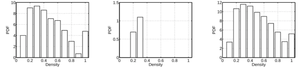
Finally, in order to give more evidences on the differences between classical and weighted models, Fig. 13 shows the density distribution of frequent connected components computed as explained in Section 4.3 (τ = 7 and σ = 6). One can see that classical models fail to create dense frequent connected components. Their density is indeed always below 0.4, which is low. On the contrary, the weighted set of models manage to reproduce a density distribution which is comparable to the one of Imote data, without having introduced this infor-mation in the models. Notice however, that the number of frequent connected subgraphs is larger in the simulated data than in the original ones. Fig. 14
0 0.2 0.4 0.6 0.8 1 0 2 4 6 8 10 Density PDF 0 0.2 0.4 0.6 0.8 1 0 0.5 1 1.5 Density PDF 0 0.2 0.4 0.6 0.8 1 0 2 4 6 8 10 12 Density PDF
Fig. 13. Density of frequent connected components for Imote (left), classical (A, middle) and weighted models (B, right)
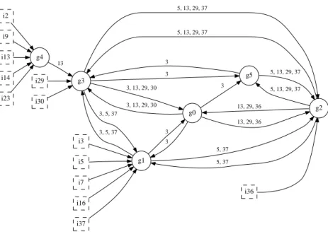
reports the trajectory of individuals among identified communities for model Cω, using the same methodology as in Section 4.3. For all classical models, it
is impossible to identify any communities satisfying the density and temporal support constraints. Because the number of frequent connected subgraphs is larger on the simulated data than on the original ones, the parameters σ and τ are increased from respectively 6 and 7 on the Imote data, to 9 and 10 on the simulated ones (see Section 4.3), so as to keep a reasonable number of com-munities. Trajectories comparable to the ones computed on Imote data are found here, once again emphasizing that weighted models are more realistic than classical ones.
6 State of the art
There exists a considerable amount of works in complex networks analysis. Network models are widely used to represent interactions between entities, such as networks from computer science (data exchange in P2P networks, chat, emails), social networks (friendship) and biological networks (infectious diseases spread). One may refer to [7] and [8] for comprehensive surveys. The field of large network analysis is relatively new (end of the 90’s). A sem-inal and famous work was certainly done by D. Watts, and Strogatz in 1998
i2 g4 g3 13 i3 g1 3, 5, 37 g2 5, 37 g0 3 i5 i7 i9 i13 i14 i16 i23 i29 3, 5, 37 5, 13, 29, 37 3, 13, 29, 30 g5 3 i30 i36 5, 37 5, 13, 29, 37 13, 29, 36 5, 13, 29, 37 i37 3 3, 13, 29, 30 13, 29, 36 3 3 5, 13, 29, 37
Fig. 14. Cω: trajectories of individuals among communities
and published in Nature [39]. Despite the title Collective dynamics of ’small-world’ networks very few is told about their dynamical properties, which would include both the study of changes of state for vertices and links, and changes of the underlying structure. Most of the recent studies in the field of complex networks (see for instance [1,16]) are focused on the topological structure of real networks, and have defined a lot of properties to properly describe these networks. Most of which are far beyond the scope of this paper. The main conclusion is that the underlying structure of complex networks has a strong impact on the propagation, i.e., the dynamic, of information or diseases [20,33]. In [34], it is shown that a dynamical property –stability or robustness against small perturbations– is highly correlated with the relative abundance of net-work motifs in several previously determined biological netnet-works. In [10], the influence of the topology on the dynamics of a system composed of very simple excitable units (modeled as a 3-state deterministic automaton) is investigated. Once more, the conclusion highlights the fact that the number of triangles and loops in the underlying topology strongly impacts the dynamics but the study of the evolution of the underlying structure was not considered. Ample work also exists on generating small world networks by using growing processes based on variants of preferential attachment [2,26]. However, such models are not appropriate for modeling the evolution of links since once a vertex or a link is created it does not evolve anymore.
One reason to explain the lack of studies fitting the needs for modeling the dynamics of complex networks, and interaction networks in particular, comes from the absence of easily observable evolving networks. Indeed, most real-world complex interaction networks are not directly available: collecting data about them requires the use of measurements and gathering experiments. Note
that measuring the dynamical aspect increases the intrinsic complexity of the such experiments [25]. Data such as the ones provided by [11], the MIT Real-ity Mining study [17] and the CRAWDAD3 are very important contributions.
These data sets are interesting as such, but they could also lead to the def-inition of new dynamical properties that could be used to validate protocol performances.
Among the few studies centered on the dynamics of networks, let us cite [3,4,38] which gives some insight on the evolution of typical subgraphs over time in different networks like the Internet, semantic or biological networks. However, these studies are based on nearly static networks where the number of time steps is extremely small, no more than a few dozens. On the contrary, the evolution of Imote or Mit data is much more complex with thousands of modifications per day. In [12], an opportunistic communication model related to both Delay-Tolerant Networking and Mobile Ad Hoc Networking is studied. From several data sets, they have observed that the inter-contact time between two devices can be approximated by a power law. The power law characteri-zation of contact and inter contacts has been used in [9] to generate synthetic traces but the authors did not analyze more complex subgraph structures and are not able to generate realistic subgraphs patterns. We emphasize that the underlying structures of the interaction networks are crucial for the study of questions regarding dynamical aspects. It has also been shown that the iden-tified topological framework may have important implications for our under-standing of the origin and function of subgraphs in all complex networks [37]. In [15], authors analyze the Mit data set and show that the topology of this network evolves over a wide range of time scales. In particular, they show that it is characterized by strong periodicities driven by external calendar cycles, and that the conversion of inherently continuous-time data into a sequence of snapshots can produce highly biased estimates of the network structure. We have not found any previous work proposing a dynamic model of interaction networks, i.e., a model taking into account the dynamics of the links in or-der to reproduce realistic synthetic traces in terms of contact / inter contact durations, of vertex degree distribution, subgraph structures, etc.
7 Conclusion & Future work
The first contribution of this paper is to propose and study a set of rigorous and coherent properties usable as a practical basis for the analysis of dynamic mobility networks that can be easily extended to large complex networks. The properties go from very basic and descriptive ones (vertices, links, degree) to
3 CRAWDAD is the Community Resource for Archiving Wireless Data At
more complex ones related to the intrinsic structure of the evolving interaction graph. We do not only extend classical notions to the dynamic case (thanks to statistical time-series analysis methodology), we also develop new notions which only make sense in dynamical context. We applied the methods and our temporal statistics on two real world interaction networks that are large in terms of measurement durations.
The key observations made using these analyses are first that all properties are highly correlated except for the links creation and deletion processes which are independent of other graph properties and second that the network can have many possible configurations, from sparse to dense. We gave strong evidence that the probability distribution of contacts and inter contacts is only one parameter for the description of interaction graphs, and definitely not the ultimate one. These results can therefore be used to build a random interaction graph simulator.
The second strong contribution is the introduction of global analyses to charac-terize the dynamics of the graph as a whole: correlation between links, stability of the connected components, number of triangles and evolution of communi-ties inside the interaction networks. An observation is that the dynamics of triangle creation is higher than what would be expected in non-structured ran-dom graphs. Another important observation is that most pairs of links have a very low correlation coefficient. Thanks to the analysis of the stability of the connected components, a better understanding of the evolution of the intrin-sic structure of interaction networks is obtained. Finally, it was shown that communities can be identified in a dynamic interaction graph, with non-trivial trajectories of individuals among them and a novel approach was proposed to find them.
Based on all the analyses performed, we are able to propose simple yet very ac-curate models that generate random interaction graphs with satisfactory tem-poral properties. The key observations made from the analysis suggest two important features: (i) links creations/deletions are independent and there-fore one could use a simulation model based on a simple Markovian links creation/removal process; (ii) intrinsic structures are not completely random: the number of triangles is important, communities are present and therefore the model should take into account these important factors in order to gener-ate similar properties. To do so, several models are proposed for the transition probabilities in a random simulator, sepcifically taking into account the ex-perimental distribution for some specific property of interest (such as the high proportion of triangles created or deleted during the dynamics). This class of models constitute a significant step towards the generation of random in-teraction graphs suitable for simulation purposes. It also points promising directions for future investigations since the model is simple and could also be used for analysis of protocol performance evaluations.
One noteworthy difference between the stationary models presented before and the real data sets is the non-stationarity. As already discussed in Section 3.2, both Imote and Mit data sets exhibit strong non-stationarity due to period-icity (day/night, week/week-end) and events (lunches, breaks, etc.). However, building non-stationary models is a complex issue, especially when doing step by step simulation. In this case it is likely that we do not have control on the simulation anymore. Nevertheless, one could define a piecewise station-ary model, but then the estimation of the empirical distributions would be of much lower quality because less data would be available. A trade-off is be to have some parameters evaluated as a function of time (at a given granularity), and others estimated on the whole data set.
Several other points remain for future extensions of this work. The dynamic community computation proposed still requires outside supervision in order to fix a threshold. Trajectories of individuals are very promising and one may imagine that such temporal and dynamic graphs may be used as a “signature” of the larger experimental data set and used as a compact temporal pattern. Finally, another point remains the crucial need for real experiments in order to validate the properties on larger data sets: larger number of participants, stronger embedded communities and longer duration. We plan to initiate such experiments and we hope that gathering further and greater in situ results will allow to deeply extend our understanding of dynamical networks.
References
[1] R. Albert, A.-L. Barabasi, Statistical mechanics of complex networks, Reviews of Modern Physics 74 (2002) 47.
[2] R. Albert, H. Jeong, A. Barabasi, The diameter of the World Wide Web, Nature 401 (1999) 130–131.
[3] M. Babu, L. Aravind, S. Teichmann, Evolutionary dynamics of prokaryotic transcriptional regulatory networks, J Mol Biol. 358 (2) (2006) 614–633. [4] M. Babu, N. Luscombe, L. Aravind, M. Gerstein, S. Teichmann, Structure and
evolution of transcriptional regulatory networks, Curr Opin Struct Biol. 14 (3) (2004) 283–291.
[5] J. Besson, C. Robardet, J.-F. Boulicaut, S. Rome, Constraint-based concept mining and its application to microarray data analysis, IDA 9 (1) (2005) 59–82. [6] B. Bollob´as, Random Graphs (2nd ed.), vol. 73 of Studies in Advanced
Mathematics, Cambridge University Press, 2001.
[7] S. Bornholdt, H. G. Schuster (eds.), Handbook of Graphs and Networks: From the Genome to the Internet, John Wiley & Sons, Inc., 2003.
[8] U. Brandes, T. Erlebach (eds.), Network Analysis: Methodological Foundations, LNCS, Springer-Verlag, 2005.
[9] R. Calegari, M. Musolesi, F. Raimondi, C. Mascolo, CTG: A connectivity trace generator for testing the performance of opportunistic mobile systems, in: Software Engineering Conference, 2007.
[10] A. Carvunis, M. Latapy, A. Lesne, C. Magnien, L. Pezard, Dynamics of three-state excitable units on poisson vs. power-law random networks, Physica A 367 (2006) 595–612.
[11] A. Chaintreau, J. Crowcroft, C. Diot, R. Gass, P. Hui, J. Scott, Pocket switched networks and the consequences of human mobility in conference environments, in: WDTN, 2005.
[12] A. Chaintreau, J. Crowcroft, C. Diot, R. Gass, P. Hui, J. Scott, Impact of human mobility on the design of opportunistic forwarding algorithms, in: INFOCOM, 2006.
[13] D. Chakrabarti, R. Kumar, A. Tomkins, Evolutionary clustering, in: KDD, ACM, 2006.
[14] Y. Chi, S. Zhu, X. Song, J. Tatemura, B. L. Tseng, Structural and temporal analysis of the blogosphere through community factorization, in: KDD, ACM Press, 2007.
[15] A. Clauset, N. Eagle, Persistence and periodicity in a dynamic proximity network, in: DIMACS Workshop, 2007.
[16] S. Dorogovtsev, J. Mendes, Evolution of networks, Adv. Phys. 51 (2002) 1079– 1187.
[17] N. Eagle, A. Pentland, Reality mining: Sensing complex social systems, Journal of Personal and Ubiquitous Computing 10 (4) (2006) 255–268.
[18] P. Erd¨ods, A. R´enyi, On random graphs, Publ. Math. (1959) 290–297.
[19] E. Fleury, J.-L. Guillaume, C. Robardet, A. Scherrer, Analysis of dynamic sensor networks: power law then what?, in: Comsware, Bengalor, India, 2007. [20] A. Ganesh, L. Massoulie, D. Towsley, The effect of network topology on the
spread of epidemics, in: INFOCOM, 2005.
[21] D. Gruhl, D. Liben-Nowell, R. V. Guha, A. Tomkins, Information diffusion through blogspace, SIGKDD Explorations 6 (2) (2004) 43–52.
[22] W. Hastings, Monte Carlo sampling methods using markov chains and their applications, Biometrika 57 (1) (1970) 97–109.
[23] D. Kempe, J. Kleinberg, E. Tardos, Maximizing the spread of influence through a social network, in: KDD, ACM Press, 2003.
[24] D. Kotz, T. Henderson, CRAWDAD: A Community Resource for Archiving Wireless Data at Dartmouth, IEEE Pervasive Computing 4 (2005) 12–14.