HAL Id: hal-00680454
https://hal.inria.fr/hal-00680454
Submitted on 20 Mar 2012
HAL is a multi-disciplinary open access
archive for the deposit and dissemination of
sci-entific research documents, whether they are
pub-lished or not. The documents may come from
teaching and research institutions in France or
abroad, or from public or private research centers.
L’archive ouverte pluridisciplinaire HAL, est
destinée au dépôt et à la diffusion de documents
scientifiques de niveau recherche, publiés ou non,
émanant des établissements d’enseignement et de
recherche français ou étrangers, des laboratoires
publics ou privés.
Codes
Pascal Véron
To cite this version:
Pascal Véron. True Dimension of Some Quadratic Binary Trace Goppa Codes. Designs, Codes and
Cryptography, Springer Verlag, 2001, 24 (1), pp.81-97. �10.1023/A:1011281431366�. �hal-00680454�
True Dimension of Some Binary Quadratic
Trace Goppa Codes
P. V ´ERON [email protected]
Groupe de Recherche en Informatique et Math´ematiques (GRIM), Universit´e de Toulon-Var, B.P. 132, 83957 La Garde Cedex, France
Communicated by: R. C. Mullin
Received May 17, 2000; Accepted September 5, 2000
Abstract. We compute in this paper the true dimension over F2of Goppa Codes !(L, g) defined by the polynomial
g(z) = TrF22s:F2s(z)proving, this way, a conjecture stated in [14,16].
Keywords: Goppa codes, trace operator, redundancy equation, parameters of Goppa codes
1. Introduction
In 1970, V. D. Goppa [8] introduced a new class of linear error-correcting codes which asymptotically meet the Varshamov-Gilbert bound: the so-called !(L, g) codes.
Definition 1. Let g(z) ∈ Fqm[z], L = {α1, . . . , αn} ⊂ Fqm such that ∀i, g(αi)%= 0. The
Goppa code !(L, g), of length n over Fq, is the set of codewords, i.e., n-tuples (c1, . . . ,cn)∈
Fnq, satisfying n ! i=1 ci z − αi ≡ 0 (mod g(z)).
The dimension k of !(L, g) and its minimal distance d satisfy
k ≥ n − m deg g(z) d ≥ deg g(z) + 1.
Other basic definitions and properties of Goppa codes are to be found in [12]. It is well known that it is a hard problem to compute the true dimension (and minimal distance) of any Goppa code. A lot of work has been done on special classes of Goppa codes in order to improve the general bound on the dimension. Notably, for (classical) Goppa codes, interested readers can refer to [1–3,5,13,14,16,17].
1.1. The Trace Goppa Codes
In [11] M. Loeloeian and J. Conan described a subclass of binary (q = 2) Goppa codes defined by g(z) = z2s
+ z and L = F22s\F2s in order to illustrate their new lower bound on
the minimum distance. In [13,14] authors studied the dimension of these codes and gave a new bound for the dimension:
dim !(L, g) ≥ n − 2s deg g(z) + 3s − 1.
This result has been generalized in [16] where a special subclass of Goppa codes has been introduced: the Trace Goppa codes.
Definition 2. Let a(z) and b(z) be two arbitrary elements of Fpms[z]. A Trace Goppa code
is a !(L, g) code where g(z) = a(z)TrFpms:Fps(b(z))and L = Fpms\{z ∈ Fpms,g(z) = 0}.
Depending on the value of p and m, three new bounds are given in [16] for the dimension of such codes. Moreover it is proved that these codes never reach the general known bound. In the so-called binary quadratic case ( p = 2, m = 2) it is shown that
dim !(L, g) ≥ n − 2s deg g(z) + 3s − 1.
For a(z) = 1 and b(z) = z, this bound corresponds to the one given in [13,14]. As mentioned in [13,16], when g(z) = TrF22s:F2s(z), the bound is reached for s = 2, 3, 4, 5. Till now, it was an open problem to know whether it was reached for all s ≥ 2.
In the quadratic case (m = 2), it is shown in [16] that: dim !(L, g) ≥ n − 2s deg g(z) + 2s − 1.
For g(z) = TrFp2s:Fps(z), it has been checked with the help of a computer that the proposed
bound is reached.
The aim of this paper is to prove that the true dimension of binary Goppa codes defined by g(z) = TrF22s:F2s(z)is n − 2s deg g(z) + 3s − 1, proving this way a conjecture stated in [14,16].
In Section 2, we recall the trace description of Goppa codes (given by Delsarte’s theorem) which makes a link between the calculation of the dimension and the number of solutions of a modular polynomial equation: the so-called redundancy equation. For the binary-quadratic case, the dimension of a trace Goppa code is equal to the number of polynomials
a(z) ∈ F22s[z] (deg a(z) < 2s) which satisfies a particular equation over F22s[z]/(z2 2s
+ z). In Section 3, we rearrange the redundancy equation as a sum of monomials which vanishes
over the polynomial ring F22s[z]. The corresponding coefficient of each monomial is either
a linear combination of the ai’s or exactly one of the ai’s (which then must be 0).
In Section 4 we seek for monomials whose corresponding coefficient is one of the ai’s
and conclude that if a(z) satisfies the redundancy equation then a(z) = a0+a1z +a2s−1z2s−1.
In Section 5, we simplify the redundancy equation by using the reduced form of a(z). This gives us three conditions over a0, a1and a2s−1.
2. Trace Description of Goppa Codes and Redundancy Equation
Let !(L, g) be an (n, k) code over F2(L ⊂ F2m), it is well known (see [12]) that it is a
restriction to F2of a generalized (n, n − deg g(z)) Reed-Solomon code ˆ! defined over F2m.
Delsarte’s theorem states that !(L, g)⊥= Tr( ˆ!⊥)where
Tr : ˆ! → Fn2
(c1, . . .cn)+→"TrF2m:F2(c1), . . . ,TrF2m:F2(cn) #
Since ˆ!⊥has dimension m deg g(z) over F2, then
n − k = dimF2!(L, g)⊥
= dimF2Im(Tr)
= m deg g(z) − dimF2ker(Tr).
A possible way to determine the dimension of a Goppa code is to compute dimF2ker(Tr).
From [14,16], in order to prove our main result we have only to show that for g(z) = TrF22s:F2s(z)and m = 2s, dimF2ker(Tr) ≤ 3s − 1.
In [13] it has been established that ker(Tr) is isomorphic to $ a(z) ∈ F22s[z] | g(z)22s−1+1TrF2s:F2% a(z) g(z) + a(z)2s g(z)2s & ≡ 0 "mod z22s+ z# ' ,
with 0 ≤ deg a(z) ≤ 2s− 1 (such an equation is obtained from the parity check matrix of
the code).
Let a(z) =(2s−1
i = 0aizi (∀i, ai∈ F22s), and g(z) = z2s+ z, since g(z)2s≡ g(z) (mod z22s + z), then g(z)22s−1+1Tr F2s:F2 % a(z) g(z) + a(z)2s g(z)2s & ≡ 0 "mod z22s# + z ⇔ g(z)2s−1+1 s−1 ! i=0 % a(z) + a(z)2s g(z) &2i ≡ 0 "mod z22s+ z# ⇔ s−1 ! i=0 "z2s + z#2s−1−2i+1 )2s−1 ! j=0 a2i jz2 ij + a2js+izj2 s+i * ≡ 0 "mod z22s+ z# PROPOSITION1. ∀i ≥ 0, "z2s + z#2s−1−2i+1 = 2s−1−i−1 ! k=0 z2s−1−2i+2ik(2s−1)+1 + 2s−1−i−1 ! k=0 z2s−1−2i+2ik(2s−1)+2s .
Proof. Let us write (z2s
+ z)2s−1−2i+1
= (z2s+ z)(z2s + z)2s−1−2i
"z2s + z#2s−1−2i = z2s−1−2i "z2s−1 + 1#2s−1−2i = z2s−1−2i"z2 s−1 + 1#2s−1 "z2s−1 + 1#2i = z2s−1−2i"z 2i(2s−1)2s−1−i + 1# "z2i(2s−1) + 1# = z2s−1−2i 2s−1−i−1 ! k=0 z2i(2s−1)k
Thus equation (1) becomes (modulo z22s
+ z) s−1 ! i=0 2s−i−1−1 ! k=0 2s−1 ! j=0 a2i j z2 s−1−2i+2ik(2s−1)+2ij+1 + s−1 ! i=0 2s−i−1−1 ! k=0 2s−1 ! j=0 a2js+iz2s−1−2i+2ik(2s−1)+2s+ij+1 + s−1 ! i=0 2s−i−1−1 ! k=0 2s−1 ! j=0 a2i j z2 s−1−2i+2ik(2s−1)+2ij+2s + s−1 ! i=0 2s−i−1−1 ! k=0 2s−1 ! j=0 a2s+i j z2 s−1−2i+2ik(2s−1)+2s+ij+2s = 0. (1)
Our main goal is to show that a necessary condition so that a polynomial a(z)
satis-fies equation (1) is that, for all j %= 0, 1, 2s−1, aj = 0. With this end in view, we are
going first to study the different degrees of the monomials which appear in the above equation.
3. Distribution of the Degrees in the Redundancy Equation • Let i = 0, since (z2s+z)2s−1−2i+1
= z22s−1+z2s−1, the degrees which appear in equation (1) are: 2s−1+ j, 2s−1+ j2s, 22s−1+ j, 22s−1+ j2sfor j = 0 . . . 2s− 1.
• Let i %= 0 the degrees can be distributed in four classes: 2s−1−2i+2ik(2s−1) + 2ij +1,
2s−1− 2i+ 2ik(2s− 1) + 2s+ij + 1, 2s−1− 2i+ 2ik(2s− 1) + 2ij + 2s, 2s−1− 2i+
2ik(2s− 1) + 2s+ij + 2s, for j = 0 . . . 2s− 1.
Now remember that we are working modulo z22s
+ z, i.e. (unformally speaking) we have
to replace 22s by 1 each time it appears.
∀ j = 0 . . . 2s− 1,
– 2s−1+ j < 22s, 2s−1+ j2s<22s, 22s−1+ j < 22s, thus these degrees remain unchanged
modulo z22s + z,
– 22s−1+ j2s <22sfor j = 0 . . . 2s−1− 1, – let j = 2s−1+ j.(0 ≤ j.≤ 2s−1− 1), then z22s−1+ j2s = z22s−1+(2s−1+ j.)2s ≡ zj.2s+1 (mod z22s + z).
∀i = 1 . . . s − 1, ∀k = 0 . . . 2s−1−i− 1, ∀ j = 0 . . . 2s− 1, let ε = 1 or 2s, – 2s−1− 2i+ 2ik(2s− 1) + 2ij + ε ≤ 2s−1− 2i+ (2s−1− 2i)(2s − 1) + 2s−1(2s − 1) + 2s ≤ 22s− 2s+1− 2s−1 <22s.
– let j = j.+ γ 2s−i, 0 ≤ j.≤ 2s−i− 1, 0 ≤ γ ≤ 2i− 1 and consider two cases:
(a) 0 ≤ j.<2s−i− k, then z2s−1−2i+2ik(2s−1)+2s+ij+ε = z2s−1−2i+2ik(2s−1)+2s+i(j.+γ 2s−i)+ε ≡ z2s−1−2i+2ik(2s −1)+2s+ij.+γ +ε "mod z22s + z# (and 2s−1− 2i+ 2ik(2s− 1) + 2s+ij.+ γ + ε < 22s).
(b) 2s−i − k ≤ j. ≤ 2s−i − 1 (remark that this occurs only for k ≥ 1). We can write
j.= j..+ 2s−i− k, 0 ≤ j..≤ k − 1. Then
z2s−1−2i+2ik(2s−1)+2s+ij+ε
= z2s−1−2i+2ik(2s−1)+2s+i(j..+2s−i−k+γ 2s−i)+ε
≡ z2s−1−2i(k+1)+2s+ij..+γ +1+ε "mod z22s
+ z#
(and 2s−1− 2i+ 2i(k + 1) + 2s+ij..+ γ + 1 + ε < 22s).
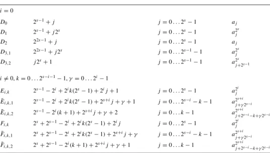
In order to sum up these results Table 1 gives for i and k fixed, the different type of degrees which appear in equation (1). In the left column we have assigned a name to each category in order to simplify the rest of the paper. Since each degree is associated to a monomial in equation (1), in the right column we list the corresponding coefficient of each monomial.
Important Remark. Set ¯Ei,k,2and ¯Fi,k,2are defined only for k ≥ 1 and i ≤ s − 2 (since
k ≤ 2s−i−1− 1).
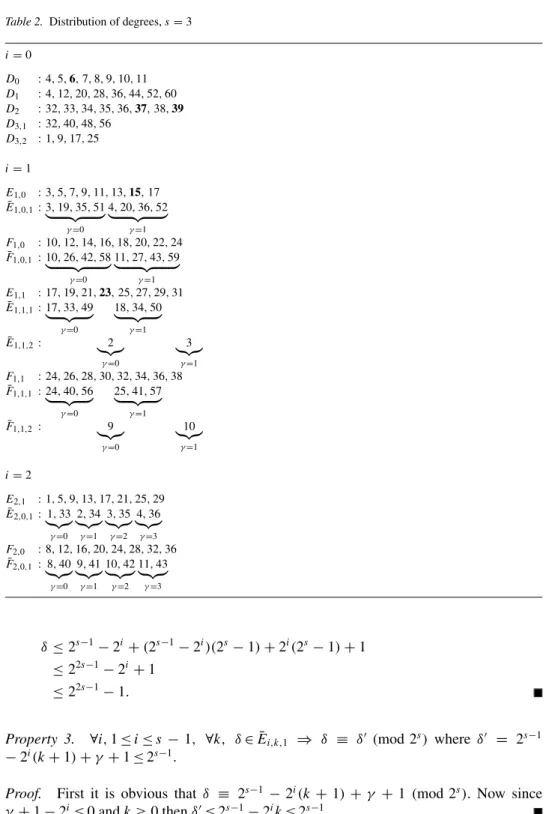
As an example, Table 2 gives the different degres which appear in equation (1) for s = 3. From now on, we have reduce equation (1) to a sum of monomials whose degrees are
less than 22s. Thus the sum of monomials vanishes over the polynomial ring F
22s[z] which implies that the corresponding coefficients are zeros. Clearly, all the sets in Table 1 are not
pairwise disjoint, otherwise all aj should be zeros and dim ker(Tr) = 0. However, for k
and i fixed, it is easy to see that each set contains distinct elements. We are now going to investigate the elements which only belong to one set for any value of i, k. Let d be such an element, then there is a single monomial of degree d in equation (1). This implies that
Table 1. Distribution of degrees i = 0 D0 2s−1+ j j = 0 . . . 2s− 1 aj D1 2s−1+ j2s j = 0 . . . 2s− 1 a2js D2 22s−1+ j j = 0 . . . 2s− 1 aj D3,1 22s−1+ j2s j = 0 . . . 2s−1− 1 a2js D3,2 j2s+ 1 j = 0 . . . 2s−1− 1 a2j+2s s−1 i %= 0, k = 0 . . . 2s−i−1− 1, γ = 0 . . . 2i− 1 Ei,k 2s−1− 2i+ 2ik(2s− 1) + 2ij + 1 j = 0 . . . 2s− 1 a2 i j
¯Ei,k,1 2s−1− 2i+ 2ik(2s− 1) + 2s+ij + γ + 1 j = 0 . . . 2s−i− k − 1 a2j+γ 2s+i s−i
¯Ei,k,2 2s−1− 2i(k + 1) + 2s+ij + γ + 2 j = 0 . . . k − 1 a2s+i
j+2s−i−k+γ 2s−i Fi,k 2s+ 2s−1− 2i+ 2ik(2s− 1) + 2ij j = 0 . . . 2s− 1 a2ji
¯Fi,k,1 2s+ 2s−1− 2i+ 2ik(2s− 1) + 2s+ij + γ j = 0 . . . 2s−i− k − 1 a2j+γ 2s+i s−i
¯Fi,k,2 2s+ 2s−1− 2i(k + 1) + 2s+ij + γ + 1 j = 0 . . . k − 1 a2j+2s+is−i−k+γ 2s−i
and must be zero. We will call such elements “isolated” degrees. In Table 2 bold integers correspond to “isolated” degrees.
4. Seeking “Isolated” Degrees
Here are some properties of the sets described in Table 1. We will often use them in the rest of the paper (we will suppose that s ≥ 3).
Property 1.
δ∈ D0⇒ δ ≤ 2s+ 2s−1− 1 (1a)
δ∈ D1⇒ δ ≡ 2s−1 (mod 2s) (and thus δ is even) (1b)
δ∈ D2⇒ 22s−1≤ δ ≤ 22s−1+ 2s− 1 (1c)
δ∈ D3,1⇒ δ ≥ 22s−1and δ ≡ 0 (mod 2i),i = 1 . . . s − 1 (1d)
δ∈ D3,2⇒ δ ≡ 1 (mod 2s) (and thus δ is odd) (1e)
Proof. All these properties are obvious.
Property 2. ∀i, 1 ≤ i ≤ s − 1, ∀ k, δ ∈ Ei,k⇒ δ ≤ 22s−1− 1 and δ ≡ 1 (mod 2i)(thus δ
is odd).
Proof. First it is obvious that δ ≡ 1 (mod 2i). Since k ≤ 2s−i−1− 1 then 2ik ≤ 2s−1− 2i.
Table 2. Distribution of degrees, s = 3 i = 0 D0 : 4, 5, 6, 7, 8, 9, 10, 11 D1 : 4, 12, 20, 28, 36, 44, 52, 60 D2 : 32, 33, 34, 35, 36, 37, 38, 39 D3,1 : 32, 40, 48, 56 D3,2 : 1, 9, 17, 25 i = 1 E1,0 : 3, 5, 7, 9, 11, 13, 15, 17 ¯E1,0,1 : 3, 19, 35, 51 + ,- . γ=0 4, 20, 36, 52 + ,- . γ=1 F1,0 : 10, 12, 14, 16, 18, 20, 22, 24 ¯F1,0,1 : 10, 26, 42, 58 + ,- . γ=0 11, 27, 43, 59 + ,- . γ=1 E1,1 : 17, 19, 21, 23, 25, 27, 29, 31 ¯E1,1,1 : 17, 33, 49 + ,- . γ=0 18, 34, 50 + ,- . γ=1 ¯E1,1,2 : 2 +,-. γ=0 3 +,-. γ=1 F1,1 : 24, 26, 28, 30, 32, 34, 36, 38 ¯F1,1,1 : 24, 40, 56 + ,- . γ=0 25, 41, 57 + ,- . γ=1 ¯F1,1,2 : 9 +,-. γ=0 10 +,-. γ=1 i = 2 E2,1 : 1, 5, 9, 13, 17, 21, 25, 29 ¯E2,0,1 : 1, 33 +,-. γ=0 2, 34 +,-. γ=1 3, 35 +,-. γ=2 4, 36 +,-. γ=3 F2,0 : 8, 12, 16, 20, 24, 28, 32, 36 ¯F2,0,1 : 8, 40 +,-. γ=0 9, 41 +,-. γ=1 10, 42 + ,- . γ=2 11, 43 + ,- . γ=3 δ≤ 2s−1− 2i+ (2s−1− 2i)(2s− 1) + 2i(2s− 1) + 1 ≤ 22s−1− 2i+ 1 ≤ 22s−1− 1.
Property 3. ∀i, 1 ≤ i ≤ s − 1, ∀k, δ ∈ ¯Ei,k,1 ⇒ δ ≡ δ.(mod 2s) where δ. = 2s−1
− 2i(k + 1) + γ + 1 ≤ 2s−1.
Proof. First it is obvious that δ ≡ 2s−1 − 2i(k + 1) + γ + 1 (mod 2s). Now since
Property 4. ∀i, 1 ≤ i ≤ s − 2, ∀k ≥ 1, δ ∈ ¯Ei,k,2 ⇒ δ ≡ δ. (mod 2s)where δ. = 2s−1
− 2i(k + 1) + γ + 2 ≤ 2s−1− 1. Moreover δ ≤ 22s−1− 2s+2+ 2s−2+ 1.
Proof. First it is obvious that δ ≡ 2s−1−2i(k +1)+γ +2 (mod 2s). Since γ +2−2i≤ 1, k ≥ 1 and i ≥ 1 then δ.≤ 2s−1−2ik+1 ≤ 2s−1−1. Moreover, since k ≤ 2s−i−1−1, j ≤ k−1
and 1 ≤ i ≤ s − 2 then
δ ≤ 2s−1− 2i2s−1−i+ 2s+i(2s−i−1− 2) + γ + 2
≤ 22s−1− 2s+2+ 2i+ 1
≤ 22s−1− 2s+2+ 2s−2+ 1.
Property 5. ∀i, 1 ≤ i ≤ s − 1, ∀k, δ ∈ Fi,k⇒ 2s≤ δ ≤ 22s−1+ 2s− 2 and δ ≡ 0 (mod 2i)
(thus δ is even).
Proof. First it is obvious that δ ≡ 0 (mod 2i). Now, since k ≥ 0, j ≥ 0 and i ≤ s − 1,
then δ ≥ 2s. Next, since 2ik ≤ 2s−1− 2i, i ≥ 1 and j ≤ 2s− 1, then
δ ≤ 2s+ 2s−1− 2i+ (2s−1− 2i)(2s− 1) + 2i(2s− 1) ≤ 22s−1+ 2s− 2i
≤ 22s−1+ 2s− 2.
Property 6. ∀i, 1 ≤ i ≤ s − 1, ∀k, δ ∈ ¯Fi,k,1⇒ δ ≡ δ. (mod 2s) where δ.= 2s−1 − 2i
(k + 1) + γ ≤ 2s−1− 1.
Proof. Proof is similar to the one of Property 3.
Property 7. ∀i, 1 ≤ i ≤ s − 2, ∀k ≥ 1, δ ∈ ¯Fi,k,2⇒ δ ≡ δ.(mod 2s)where δ.= 2s−1− 2i
(k + 1) + γ + 1 ≤ 2s−1− 2. Moreover δ ≤ 22s−1− 2s+2+ 2s+ 2s−2.
Proof. Proof is similar to the one of Property 4. We can now specify which degrees are “isolated.”
LEMMA1. ∀i = 1 . . . s − 1, ∀k, ∀ j, 2 ≤ j ≤ 2s−1− 1, j even
2s−1+ j ∈ D
0
2s−1+ j /∈ D
1∪ D2∪ D3,1∪ D3,2∪ Ei,k∪ ¯Ei,k,1∪ ¯Ei,k,2∪ Fi,k ∪ ¯Fi,k,1∪ ¯Fi,k,2
Proof. Let & = 2s−1+ j, notice that
• &is even,
• 2s−1< & <2s(thus & remains unchanged modulo 2s).
From Propositions 2 and 5, ∀i = 1 . . . s − 1, ∀k, & /∈ Ei,k∪ Fi,k.
From Propositions 3, 4 and 6, 7, ∀i = 1 . . . s−1, ∀k ≥ 1, & /∈ ¯Ei,k,1∪ ¯Ei,k,2∪ ¯Fi,k,1∪ ¯Fi,k,2.
LEMMA2. ∀i = 1 . . . s − 1, ∀k, ∀ j, 2s−1+ 1 ≤ j ≤ 2s− 1, j odd
22s−1+ j ∈ D2
22s−1+ j /∈ D
0∪ D1∪ D3,1∪ D3,2∪ Ei,k∪ ¯Ei,k,1∪ ¯Ei,k,2∪ Fi,k∪ ¯Fi,k,1∪ ¯Fi,k,2
Proof. Let & = 22s−1+ j, then:
• &is odd,
• &≡ j (mod 2s), j ≥ 2s−1+ 1,
• 22s−1≤ & ≤ 22s−1+ 2s− 1.
From Propositions 1a, 1b, 1d and 1e, & /∈ D0∪ D1∪ D3,1∪ D3,2.
From Propositions 2 and 5, ∀i = 1 . . . s − 1, ∀k, & /∈ Ei,k∪ Fi,k.
From Propositions 3, 4 and 6, 7, ∀i = 1 . . . s − 1, ∀k, & /∈ ¯Ei,k,1∪ ¯Ei,k,2∪ ¯Fi,k,1∪ ¯Fi,k,2.
LEMMA3. ∀ j, 3 ≤ j ≤ 2s−2+ 1, j odd
• 2s+1+ 2s−1+ 2 j − 3 ∈ E
1,1,
• ∀k %= 1, 2s+1+ 2s−1+ 2 j − 3 /∈ E1,k,
• ∀i > 1, ∀k, 2s+1+ 2s−1+ 2 j − 3 /∈ Ei,k,
• ∀i ≥ 1, ∀k, 2s+1+ 2s−1+ 2 j − 3 /∈ D0∪ D1∪ D2∪ D3,1∪ D3,2∪ ¯Ei,k,1∪ ¯Ei,k,2∪ Fi,k∪
¯Fi,k,1∪ ¯Fi,k,2.
Proof. Let & = 2s+1+ 2s−1+ 2 j − 3, notice that:
• &is odd,
• 2s+1+ 2s−1+ 3 ≤ & ≤ 2s+1+ 2s− 1.
Moreover, & ≡ 2s−1+ 2 j − 3 (mod 2s), and
1 < 2s−1+ 3 ≤ 2s−1+ 2 j − 3 ≤ 2s
− 1.
From Propositions 1a, 1b, 1c, 1d and 1e, & /∈ D0∪ D1∪ D2∪ D3,1∪ D3,2.
Let i = 1 and k = 0, then δ ∈ E1,0⇒ ∃ j., 0 ≤ j.≤ 2s− 1, such that δ = 2s−1+ 2 j.−
1 ≤ 2s+1+ 2s−1− 3 < &. Thus & /∈ E1,0.
From Proposition 2, if ∀i > 1, & %≡ 1 (mod 2i)then & /∈ E
i,k (for any value of k). Now,
∀i > 1, & ≡ 2 j − 3 (mod 2i), thus
2 j − 3 ≡ 1 (mod 2i)
⇒ j ≡ 2 (mod 2i−1),
which is impossible since j is odd.
From Proposition 5, ∀i = 1 . . . s − 1, ∀k, & /∈ Fi,k.
From Propositions 3, 4 and 6, 7, ∀i = 1 . . . s − 1, ∀k, & /∈ ¯Ei,k,1∪ ¯Ei,k,2∪ ¯Fi,k,1∪ ¯Fi,k,2.
LEMMA4. ∀ j, 2s−2+ 3 ≤ j ≤ 2s−1− 1, j odd
• 2s+1j + 2s−1− 1 ∈ ¯E1,0,1(for γ = 0),
• ∀k %= 0, 2s+1j + 2s−1− 1 /∈ ¯E1,k,1,
• ∀i > 1, ∀k, 2s+1j + 2s−1− 1 /∈ ¯Ei,k,1,
• ∀i = 1 . . . s − 1, ∀k, 2s+1j + 2s−1− 1 /∈ D0∪ D1∪ D2∪ D3,1∪ D3,2∪ Ei,k∪ ¯Ei,k,2∪ Fi,k
∪ ¯Fi,k,1∪ ¯Fi,k,2.
Proof. Let & = 2s+1j + 2s−1− 1, notice that:
• &is odd,
• &≡ 2s−1− 1 (mod 2s),
• 22s−1+ 2s+2+ 2s+1+ 2s−1− 1 ≤ & ≤ 22s− 2s+1+ 2s−1− 1,
• 2 &
2s+13 = j is odd.
From Propositions 1a, 1b, 1c, 1d and 1e, & /∈ D0∪ D1∪ D2∪ D3,1∪ D3,2.
From Propositions 2 and 5, ∀i = 1 . . . s − 1, ∀k, & /∈ Ei,k∪ Fi,k.
Let k %= 0, δ ∈ ¯E1,k,1⇒ δ ≡ 2s−1− 2k + γ − 1 (mod 2s). Thus if 2s−1− 2k + γ − 1
%= 2s−1− 1 then & /∈ ¯E1,k,1. Now
2s−1− 2k + γ − 1 = 2s−1− 1 ⇔ γ = 2k.
Since i = 1, then γ ≥ 0 and γ ≤ 1, hence there is a unique solution to the above equation:
k = γ = 0. Thus, ∀k %= 0, & /∈ ¯E1,k,1.
Let i ≥ 2 then, ∀k, δ ∈ ¯Ei,k,1⇒ ∃ j., γ, such that
δ
2s+1 = 2i−1(k + j.)+
2s−1− 2ik + γ + 1 − 2i
2s+1 .
Now since γ + 1 − 2i≤ 0 and k ≥ 0, then
Moreover since 2ik ≤ 2s−1− 2i and γ ≥ 0, then
2s−1− 2ik + γ + 1 − 2i≥ 1.
Hence
0 < 2s−1− 2ik + γ + 1 − 2i
2s+1 <1.
Thus ∀i ≥ 2, ∀k, δ ∈ ¯Ei,k,1⇒ 22s+1δ 3 is even. Hence & /∈ ¯Ei,k,1.
∀i = 1 . . . s − 1, ∀k, let δ ∈ ¯Fi,k,1, then δ ≡ δ.(mod 2s+1), where δ. = 2s+ 2s−1− 2i
(k +1)+γ . Since γ ≥ 0 and k +1 ≤ 2s−i−1, then δ.≥ 2s. Now & ≡ 2s−1−1 (mod 2s+1), hence & /∈ ¯Fi,k,1.
From Propositions 4 and 7, ∀i = 1 . . . s − 2, ∀k ≥ 1, & /∈ ¯Ei,k,2∪ ¯Fi,k,2.
LEMMA5. ∀ j, 2s−1+ 2 ≤ j ≤ 2s−1+ 2s−2, j even
• 2s−1+ 2 j − 1 ∈ E1,0,
• ∀k ≥ 1, 2s−1+ 2 j − 1 /∈ E1,k,
• ∀i > 1, ∀k, 2s−1+ 2 j − 1 /∈ Ei,k,
• ∀i = 1 . . . s − 1, ∀k, 2s−1+ 2 j − 1 /∈ D0∪ D1∪ D2∪ D3,1∪ D3,2∪ ¯Ei,k,1∪ ¯Ei,k,2∪ Fi,k
∪ ¯Fi,k,1∪ ¯Fi,k,2.
Proof. Let & = 2s−1+ 2 j − 1, notice that:
• &is odd,
• 2s+ 2s−1+ 3 ≤ & ≤ 2s+1− 1,
• let us write j = 2s−1+ j., 2 ≤ j.≤ 2s−2, j.even. Then & ≡ 2s−1+ 2 j.− 1 (mod 2s),
and 2s−1+ 2 j.− 1 ≥ 2s−1+ 3 > 1.
From Propositions 1a, 1b, 1c, 1d and 1e, & /∈ D0∪ D1∪ D2∪ D3,1∪ D3,2.
∀k ≥ 1, let δ ∈ E1,k, then δ ≥ 2s−1− 1 + 2(2s− 1) > &, thus & /∈ E1,k.
From Proposition 2, if ∀i > 1, & %≡ 1 (mod 2i)then & /∈ E
i,k (for any value of k). Now
∀i > 1, & ≡ 2 j − 1 (mod 2i), and
2 j − 1 ≡ 1 (mod 2i)
⇒ j ≡ 1 (mod 2i−1),
which is impossible since j is even.
From Proposition 5, ∀i, 1 ≤ i ≤ s − 1, ∀k, & /∈ Fi,k.
From Propositions 3, 4 and 6, 7, ∀i, 1 ≤ i ≤ s − 1, ∀k, & /∈ ¯Ei,k,1∪ ¯Ei,k,2∪ ¯Fi,k,1∪ ¯Fi,k,2.
• (j + 1)2s+1+ 2s−1− 2 ∈ ¯E1,1,1(for γ = 1),
• ∀k %= 1, ( j + 1)2s+1+ 2s−1− 2 /∈ ¯E1,k,1,
• ∀i > 1, ∀k, ( j + 1)2s+1+ 2s−1− 2 /∈ ¯Ei,k,1,
• ∀i = 1 . . . s − 1, ∀k, ( j + 1)2s+1+ 2s−1− 2 /∈ D0∪ D1∪ D2∪ D3,1∪ D3,2∪ Ei,k∪ ¯Ei,k,2
∪ Fi,k∪ ¯Fi,k,1∪ ¯Fi,k,2.
Proof. Let & = ( j + 1)2s+1+ 2s−1− 2, notice that:
• &is even,
• &≡ 2s−1− 2 (mod 2s),
• 22s−1+ 2s+2+ 2s+1+ 2s−1− 2 ≤ & ≤ 22s− 2s+1+ 2s−1− 2,
• 2 &
2s+13 = j + 1 is odd.
From Propositions 1a, 1b and 1c, & /∈ D0∪ D1∪ D2.
Let δ ∈ D3,1, then δ ≡ 0 (mod 2s), thus & /∈ D3,1.
From Proposition 1e, & /∈ D3,2.
From Propositions 2 and 5, ∀i = 1 . . . s − 1, ∀k, & /∈ Ei,k∪ Fi,k.
Let k %= 1, δ ∈ ¯E1,k,1 ⇒ δ ≡ 2s−1− 2k + γ − 1 (mod 2s). Thus if 2s−1− 2k + γ − 1
%= 2s−1− 2 then & /∈ ¯E1,k,1. Now
2s−1− 2k + γ − 1 = 2s−1− 2 ⇔ γ = 2k − 1.
Since i = 1, then γ ≥ 0 and γ ≤ 1, hence there is a unique solution to the above equation:
k = γ = 1. Thus, ∀k %= 1, & /∈ ¯E1,k,1.
Let i ≥ 2 then, ∀k, δ ∈ ¯Ei,k,1⇒ ∃ j., γ, such that
δ 2s+1 = 2i−1(k + j.)+ 2s−1− 2ik + γ + 1 − 2i 2s+1 . Since 0 < 2s−1− 2ik + γ + 1 − 2i 2s+1 <1,
(see proof of lemma 4), 2 δ
2s+13 is even and thus ∀i ≥ 2, ∀k, & /∈ ¯Ei,k,1.
∀i = 1 . . . s − 1, ∀k, let δ ∈ ¯Fi,k,1, then δ ≡ δ.(mod 2s+1), where δ.= 2s+ 2s−1− 2i(k +
1) + γ . Since γ ≥ 0 and k + 1 ≤ 2s−i−1, then δ.≥ 2s. Now & ≡ 2s−1− 2 (mod 2s+1),
hence & /∈ ¯Fi,k,1.
5. The Reduced Redundancy Equation
PROPOSITION2. Let a(z) =(2i=0s−1aizibe a polynomial of degree at most2s− 1. If a(z) satisfies the redundancy equation (1) then, ∀i %= 0, 1, 2s−1, a
i= 0. Proof. From Table 1:
• coefficients aj are associated to monomials whose degree belongs to D0, thus from
Lemma 1, ∀ j, 2 ≤ j ≤ 2s−1− 1, j even, a
j = 0,
• coefficients aj are associated to monomials whose degree belongs to D2, thus from
Lemma 2, ∀ j, 2s−1+ 1 ≤ j ≤ 2s− 1, j odd, a
j = 0,
• coefficients a2
j are associated to monomials whose degree belongs to E1,1, thus from
Lemma 3, ∀ j, 3 ≤ j ≤ 2s−2+ 1, j odd, a2
j = 0, which implies aj = 0
• coefficients a2s+1
j are associated to monomials whose degree belongs to ¯E1,0,1(for γ = 0),
thus from Lemma 4, ∀ j, 2s−2+3 ≤ j ≤ 2s−1−1, j odd, a2s+1
j = 0, which implies aj = 0,
• coefficients a2
j are associated to monomials whose degree belongs to E1,0 , thus from
Lemma 5, ∀ j, 2s−1+ 2 ≤ j ≤ 2s−1+ 2s−2, j even, a2
j = 0, which implies aj = 0,
• coefficients a2s+1
j+2s−1 are associated to monomials whose degree belongs to ¯E1,1,1 (for
γ = 1), thus from Lemma 6, ∀ j, 2s−2+ 2 ≤ j ≤ 2s−1− 2, j even, a2j+2s+1s−1 = 0, which
implies aj = 0, ∀ j, 2s−1+ 2s−2+ 2 ≤ j ≤ 2s− 2, j even.
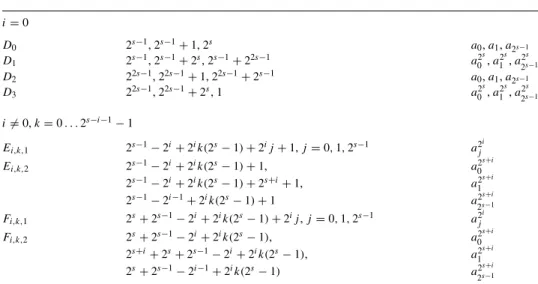
Hence, if a polynomial a(z) satisfies equation (1) then a(z) = a0+ a1z + a2s−1z2s−1. This
gives us a new distribution of degrees which appear in equation (1). We can now distribute them in 8 classes as shown in Table 3. We are now going to deduce, from this “reduced” redundancy equation, some properties over a0, a1and a2s−1, in order to prove our main result.
PROPOSITION3. Let & = 2s−1, then – & ∈ D0∪ D1∪ E1,0,2,
– ∀k %= 0, & /∈ E1,k,2,
– ∀i ≥ 2, ∀k, & /∈ Ei,k,2,
– ∀i, 1 ≤ i ≤ s − 1, ∀k, & /∈ D2∪ D3∪ Ei,k,1∪ Fi,k,1∪ Fi,k,2.
Proof. Obviously, & /∈ D2∪ D3. ∀i, 1 ≤ i ≤ s − 1, ∀k, all elements of Ei,k,1are odd, thus
& /∈ Ei,k,1.
Let i = 1 and k %= 0, then all elements of E1,k,2are greater than 2s, hence & /∈ E1,k,2.
Let i ≥ 2, ∀k, all elements of Ei,k,2are odd, thus & /∈ Ei,k,2.
∀i, 1 ≤ i ≤ s − 1, ∀k,
δ∈ Fi,k,1∪ Fi,k,2⇒ δ ≥ 2s+ 2s−1− 2i≥ 2s > &
Table 3. Reduced redundancy equation i = 0 D0 2s−1, 2s−1+ 1, 2s a0, a1, a2s−1 D1 2s−1, 2s−1+ 2s, 2s−1+ 22s−1 a02s, a2 s 1 , a2 s 2s−1 D2 22s−1, 22s−1+ 1, 22s−1+ 2s−1 a0, a1, a2s−1 D3 22s−1, 22s−1+ 2s, 1 a02s, a2 s 1 , a2 s 2s−1 i %= 0, k = 0 . . . 2s−i−1− 1 Ei,k,1 2s−1− 2i+ 2ik(2s− 1) + 2ij + 1, j = 0, 1, 2s−1 a2ji Ei,k,2 2s−1− 2i+ 2ik(2s− 1) + 1, a02s+i 2s−1− 2i+ 2ik(2s− 1) + 2s+i+ 1, a2s+i 1 2s−1− 2i−1+ 2ik(2s− 1) + 1 a2s+i 2s−1 Fi,k,1 2s+ 2s−1− 2i+ 2ik(2s− 1) + 2ij, j = 0, 1, 2s−1 a2ji Fi,k,2 2s+ 2s−1− 2i+ 2ik(2s− 1), a02s+i 2s+i+ 2s+ 2s−1− 2i+ 2ik(2s− 1), a2s+i 1 2s+ 2s−1− 2i−1+ 2ik(2s− 1) a2s+i 2s−1
COROLLARY1. Let a(z) be a polynomial which satisfies equation (1), then
a22s−1s+1= TrF22s:F2s(a0).
Proof. The sum of the coefficients of the monomials of degree 2s−1 which appear in
equation (1) must be zero. From the above proposition there are exactly three monomials of
degree 2s−1in equation (1) whose corresponding coefficients are : a
0(D0), a2
s
0 (D1), a22s+1s−1
(E1,0,2). Thus, we conclude that a0+ a2
s
0 + a22s+1s−1 = 0.
PROPOSITION4. Let & = 2s+1+ 2s−1− 1, then
– & ∈ E1,1,1∪ E1,0,2,
– ∀k %= 1, & /∈ E1,k,1,
– ∀k %= 0, & /∈ E1,k,2,
– ∀i ≥ 2, ∀k, & /∈ Ei,k,1∪ Ei,k,2,
– ∀i, 1 ≤ i ≤ s − 1, ∀k, & /∈ D0∪ D1∪ D2∪ D3∪ Fi,k,1∪ Fi,k,2.
Proof. Clearly, & /∈ D0∪ D1∪ D2∪ D3.
Let δ ∈ Ei,k,1, (i, k) %= (1, 1),
– let i ≥ 2, then δ ≡ 1 (mod 2i). Now & ≡ −1 (mod 2i),
– let i = 1 and k %= 1, then since δ = 2s+1k + 2s−1+ 2( j − k − 1),
• δ <2s+ 2s−1− 2 < & (k = 0),
Hence ∀i, 1 ≤ i ≤ s − 1, ∀k, i %= 1 or k %= 1, & /∈ Ei,k,1.
Let δ ∈ Ei,k,2, (i, k) %= (1, 0), δ takes three values:
– δ = 2s−1− 2i+ 2ik(2s− 1) + 1. Then δ ≡ δ. (mod 2s − 1), where δ. = 2s−1− 2i
+ 1 ≤ 2s−1− 1. Now & ≡ 2s−1+ 1 (mod 2s− 1).
– δ = 2s−1− 2i+ 2ik(2s− 1) + 2s+i+ 1
• let i = 1 and k ≥ 1, then δ = 2s+1+ 2s−1+ 2k(2s− 1) − 1 > &,
• let i ≥ 2, then (since 2i≤ 2s−1) δ ≥ 2s+2+ 1 > &.
– δ = 2s−1− 2i−1+ 2ik(2s− 1) + 1. Then δ ≡ δ. (mod 2s− 1), where δ.= 2s−1− 2i−1
+ 1 ≤ 2s−1.
Hence ∀i, 1 ≤ i ≤ s − 1, ∀k, i %= 1 or k %= 0, & /∈ Ei,k,2.
∀i, 1 ≤ i ≤ s − 1, ∀k, all elements of Fi,k,1are even, thus & /∈ Fi,k,1.
∀i, 2 ≤ i ≤ s − 1, ∀k, all elements of Fi,k,2are even, thus & /∈ Fi,k,2.
Let i = 1, ∀k, the first two elements of F1,k,2are even and the third one is equal to 2s−1
modulo 2s− 1, hence & /∈ F 1,k,2.
COROLLARY2. Let a(z) be a polynomial which satisfies equation (1), then a1∈ F2s.
Proof. The sum of the coefficients of the monomials of degree 2s+1+ 2s−1− 1 which
appear in equation (1) must be zero. From the above proposition there are exactly two
monomials of degree 2s+1+ 2s−1− 1 in equation (1) whose corresponding coefficients are :
a2
1 (E1,1,1,j = 1) and a12s+1(E1,0,2). Thus, we conclude that
a2s+1
1 + a21= 0
⇒ TrF22s:F2s(a1)= 0 ⇒ a1∈ F2s.
PROPOSITION5. Let & = 2s−1+ 1, then
– ∀i, 1 ≤ i ≤ s − 1, 2s−1+ 1 ∈ D
0∪ Ei,0,1,
– ∀i, 1 ≤ i ≤ s − 1, ∀k %= 0, 2s−1+ 1 /∈ E i,k,1,
– ∀i, 1 ≤ i ≤ s − 1, ∀k, 2s−1+ 1 /∈ D
1∪ D2∪ D3∪ Ei,k,2∪ Fi,k,1∪ Fi,k,2.
Proof. Clearly & /∈ D1∪ D2∪ D3. ∀i, 1 ≤ i ≤ s − 1, ∀k ≥ 1, let δ ∈ Ei,k,1 then δ ≥ 2s+1
− 1 > &, hence & /∈ Ei,k,1.
∀i, 1 ≤ i ≤ s − 1, ∀k, let δ ∈ Ei,k,2, then δ takes three values:
– δ = 2s−1− 2i+ 2ik(2s− 1) + 1, hence δ ≡ δ. (mod 2s− 1), where δ. = 2s−1− 2i
+ 1 ≤ 2s−1− 1 < &,
– δ = 2s−1− 2i+ 2ik(2s− 1) + 2s+i+ 1 = & + 2s+i+ 2ik(2s− 1) − 2i> &,
– δ = 2s−1− 2i−1+ 2ik(2s− 1) + 1, hence δ ≡ δ. (mod 2s− 1), where δ.= 2s−1− 2i−1
Hence ∀i, 1 ≤ i ≤ s − 1, ∀k, & /∈ Ei,k,2.
∀i, 1 ≤ i ≤ s − 1, ∀k, all elements of Fi,k,1are even, thus & /∈ Fi,k,1.
∀i, 2 ≤ i ≤ s − 1, ∀k, all elements of Fi,k,2are even, thus & /∈ Fi,k,2.
Let i = 1, ∀k, the first two elements of F1,k,2are even and the third one is equal to 2s−1
modulo 2s− 1, hence & /∈ F 1,k,2.
COROLLARY3. Let a(z) be a polynomial which satisfies equation (1), then
TrF2s:F2(a1)= 0.
Proof. The sum of the coefficients of the monomials of degree 2s−1+ 1 which appear
in equation (1) must be zero. From the above proposition there are exactly s monomials
of degree 2s−1+ 1 in equation (1) whose corresponding coefficients are : a
1(D0) and a2
i
1
(Ei,0,1,j = 1, 1 ≤ i ≤ s − 1). Thus, we conclude that: s−1
!
i=0 a2i
1 = 0.
6. The Main Result
THEOREM1. Let g(z) = TrF22s:F2s(z) and L = F22s\F2s, the dimension of the Goppa code
!(L, g) satisfies:
dim !(L, g) = n − 2s deg g(z) + 3s − 1.
Proof. From [13, 16], it is already known that dim !(L, g) ≥ n − 2s deg g(z) + 3s − 1. Moreover, from trace description of Goppa codes (see §2), we know that:
dim !(L, g) = n − 2s deg g(z) + dimF2ker(Tr).
From [13], ker(Tr) is isomorphic to the set I equal to: {a(z) ∈ F22s[z] | g(z)2s−1+1TrF 2s:F2 % a(z) + a(z)2s g(z) & ≡ 0 (mod z22s+ z)}.
From Proposition 2, if a(z) ∈ I , then a(z) = a0+ a1z + a2s−1z2s−1. From Corollary 1,
a2s−1is an element of the subfield F2sand for any given a2s−1∈ F2s, there are 2svalues of a0
which satisfies TrF22s:F2s(a0)= a2
s+1
2s−1. From Corollary 2, a1∈ F2s, and (from Corollary 3),
TrF2s:F2(a1)= 0. Therefore, there are exactly 2s−1elements which satisfy such conditions.
This means that I has at most 2s2s−12s distinct elements a(z). We concluded that
dimF2ker(Tr) ≤ 3s − 1.
In Table 4, we give for s = 3 and s = 4, the parameters of the associate trace Goppa code. First column contains n, k, d (d being the classical lower bound on the minimal distance)
and ¯dwhich is the minimal distance computed by a probabilistic algorithm [6]. For s = 3, ¯d
is the true minimal distance of the code. The middle column gives for n and k fixed the lower and upper bound on the minimum distance of a binary linear code as mentioned in [9]. The
Table 4. !(L, g) Linear Non-Linear (n, k, d, ¯d) (n, k, dmin,dmax) (n, r, d) s = 3 (56, 16, 18, 20) (56, 16, 20, 20) (56, 17, 20) s = 4 (240, 123, 34, 36) (240, 123, 32, 52) (240, 132, 30)
right column gives for n and d fixed, the value n − r of the best known non-linear binary
code C (as found in [9]) where r = n −log2card(C) is the so-called redundancy of the code.
Remark. It has been proved in [16], that codewords of trace Goppa codes have only even weight, which increases by 1 the general lower bound on the minimum distance.
References
1. S. V. Bezzateev and E. T. Mironchikov, N. A. Shekhunova, One subclass of binary Goppa codes, Proc. XI Simp. po Probl. Izbit. v Inform. Syst.(1986) pp. 140–141.
2. S. V. Bezzateev and N. A. Shekhunova, On the subcodes of one class Goppa Codes, Proc. Intern. Workshop Algebraic and Combinatorial Coding Theory ACCT-1(1988) pp. 143–146.
3. S. V. Bezzateev, E. T. Mironchikov and N. A. Shekhunova, A Subclass of Binary Goppa Code, Problemy Peredachi Informatsii, Vol. 25, No. 3 (1989) pp. 98–102.
4. S. V. Bezzateev and N. A. Shekhunova, Subclass of Binary Goppa Codes with Minimal Distance Equal to the Design Distance, IEEE Trans. Info. Theory, Vol. 41, No 2 (1995) pp. 554–555.
5. S. V. Bezzateev and N. A. Shekhunova, A subclass of binary Goppa codes with improved estimation of the code dimension, Design, Codes and Cryptography, Vol. 14, No. 1 (1998) pp. 23–38.
6. A. Canteaut and F. Chabaud, A new algorithm for finding minimum-weight words in a linear code: Application to McEliece’s cryptosystem and to narrow-sense BCH codes of length 511, IEEE Trans. Info. Theory, Vol. 44, No. 1 (1998) pp. 367–378.
7. P. Delsarte, On subfield subcodes of modified reed-solomon codes, IEEE Trans. Info. Theory, Vol. IT-21 (1975) pp. 575–576.
8. V. D. Goppa, A new class of linear error correcting codes, Probl. Pered. Inform., Vol. 6, (1970) pp. 24–30. 9. V.S. Pless and W.C. Huffman (eds.), Handbook of Coding Theory, Vol. 1, North Holland, 1998.
10. J. M. Jensen, Subgroup subcodes, IEEE Trans. Info. Theory, Vol. 41, No. 3 (1995) pp. 781–785.
11. M. Loeloeian, J.Conan, A transform approach to goppa codes, IEEE Trans. Info. Theory, Vol. IT-33 (1987) pp. 105–115.
12. F. J. Mac Williams and N. J. A. Sloane, The Theory of Error Correcting Codes, North Holland (1983). 13. A. M. Roseiro, The Trace Operator and Generalized Goppa Codes, Ph.D. Dissert., Dept. of Elect. Eng.,
Michigan State Univ., East Lansing, MI 48823 (1989).
14. A. M. Roseiro, J. I. Hall, J. E. Hadney, M. Siegel, The trace operator and redundancy of Goppa codes, IEEE Trans. Info. Theory., Vol. 38, No 3. (1992) pp. 1130–1133.
15. H. Stichtenoth, On the dimension of subfield subcodes, IEEE Trans. Info. Theory., Vol. 36 (1990) pp. 90–93. 16. P. V´eron, Goppa codes and trace operator, IEEE Trans. Info. Theory, Vol. 44, No. 1 (1998) pp. 290–295. 17. M. van der Vlugt, The true dimension of certain binary Goppa codes, IEEE Trans. Info. Theory., Vol. 36,
No. 2, (1990) pp. 397–398..
18. M. van der Vlugt, On the dimension of trace codes, IEEE Trans. Info. Theory., Vol. 37, No. 1 (1991) pp. 196–199.