Book Principle Of Physics pdf - Web Education

(1)

(2)

PRINCIPLES

OF PHYSICS

From Quantum Field Theory to Classical Mechanics

(3)

Series Editor: Bangfen Zhu (Tsinghua University, China)

Vol. 1 Möbius Inversion in Physics by Nanxian Chen

Vol. 2 Principles of Physics — From Quantum Field Theory to Classical Mechanics

(4)

N E W J E R S E Y • L O N D O N • S I N G A P O R E • B E I J I N G • S H A N G H A I • H O N G K O N G • TA I P E I • C H E N N A I

World Scientific

TSINGHUA

Report and Review in

Physics Vol. 2

PRINCIPLES

OF PHYSICS

Ni Jun

Tsinghua University, China

From Quantum Field Theory

to Classical Mechanics

(5)

World Scientific Publishing Co. Pte. Ltd. 5 Toh Tuck Link, Singapore 596224

USA office: 27 Warren Street, Suite 401-402, Hackensack, NJ 07601 UK office: 57 Shelton Street, Covent Garden, London WC2H 9HE

British Library Cataloguing-in-Publication Data

A catalogue record for this book is available from the British Library.

Tsinghua Report and Review in Physics — Vol. 2 PRINCIPLES OF PHYSICS

All rights reserved. This book, or parts thereof, may not be reproduced in any form or by any means, electronic or mechanical, including photocopying, recording or any information storage and retrieval system now known or to be invented, without written permission from the publisher.

For photocopying of material in this volume, please pay a copying fee through the Copyright Clearance Center, Inc., 222 Rosewood Drive, Danvers, MA 01923, USA. In this case permission to photocopy is not required from the publisher.

ISBN 978-981-4579-39-1

(6)

October 17, 2013 16:1 BC: 9056 - Principle of Physics ws-book9x6junni

To my daughter Ruyan

(7)

(8)

Preface

During the 20th century, physics experienced a rapid expansion. A gen-eral theoretical physics curriculum now consists of a collection of separate courses labeled as classical mechanics, electrodynamics, quantum mechan-ics, statistical mechanmechan-ics, quantum field theory, general relativity, etc., with each course taught in a different book. I consider there is a need to write a book which is compact and merge these courses into one single unified course. This book is an attempt to realize this aim. In writing this book, I focus on two purposes. (1) Historically, physics is established from classical mechanics to quantum mechanics, from quantum mechanics to quantum field theory, from thermodynamics to statistical mechanics, and from New-tonian gravity to general relativity. However, a more logical subsequent presentation is from quantum field theory to classical mechanics, and from the physics principles on the microscopic scale to physics on the macro-scopic scale. In this book, I try to achieve this by elucidating the physics from quantum field theory to classical mechanics from a set of common ba-sic principles in a unified way. (2) Phyba-sics is considered as an experimental science. This view, however, is being changed. In the history of physics, there are two epic heroes: Newton and Einstein. They represent two epochs in physics. In the Newtonian epoch, physical laws are deduced from exper-imental observations. People are amazed that the observed physical laws can be described accurately by mathematical equations. At the same time, it is reasonable to ask why nature should obey the physical laws described by the mathematical equations. After wondering how accurately nature obeys the gravitational law that the gravitation force is proportional to the inverse square of the distance, one would ask why it is not found in other ways. Einstein creates a new epoch by deducing physical laws not merely from experiments but also from principles such as simplicity, symmetry

(9)

viii Principles of Physics

and other understandable credos. From the view of Einstein, physical laws should be natural and simple. It is my belief that all physics laws should be understandable. In this book, I endeavor to establish the physical for-malisms based on basic principles that are as simple and understandable as possible.

The book covers all the disciplines of fundamental physics, including quantum field theory, quantum mechanics, statistical mechanics, thermo-dynamics, general relativity, electromagnetic field, and classical mechanics. Instead of the traditional pedagogic way, the subjects and formalisms are arranged in a logical-sequential way, i.e. all the formulas are derived from the formulas before them. The formalisms are also kept self-contained, i.e. the derivations of all the physical formulas which appear in this book can be found in the same book. Most of the required mathematical tools are also given in the appendices. Although this book covers all the disciplines of fundamental physics, the book is compact and has only about 400 pages because the contents are concise and can be treated as an integrated entity. In this book, the main emphasis is the basic formalisms of physics. The topics on applications and approximation methods are kept to a minimum and are selected based on their generality and importance. Still it was not easy to do it when some important topics had to be omitted. Since it is impossible to provide an exhaustive bibliography, I list only the related textbooks and monographs that I am familiar with. I apologize to the authors whose books have not been included unintentionally.

This book may be used as an advanced textbook by graduate students. It is also suitable for physicists who wish to have an overview of fundamental physics.

I am grateful to all my colleagues and students for their inspiration and help. I would also like to express my gratitude to World Scientific for the assistance rendered in publishing this book.

Jun Ni August 8, 2013 Tsinghua, Beijing

(10)

6.4 The operator of time translation in quantum mechanics . 175 6.5 Transformation of basis . . . 177 6.6 One-body operators . . . 181 6.7 Schr¨odinger equation . . . 183 7. Electromagnetic Field 187 7.1 Current density . . . 187 7.2 Classical limit . . . 189 7.3 Maxwell equations . . . 190 7.4 Gauge invariance . . . 191

7.5 Radiation of electromagnetic waves . . . 191

7.6 Poisson equation . . . 193

7.7 Electrostatic energy of charges . . . 194

7.8 Many-body operators . . . 195

7.9 Potentials of charge particles in the classical limit . . . . 197

8. Quantum Mechanics 199 8.1 Equations of motion for operators in quantum mechanics 199 8.1.1 Ehrenfest’s theorem . . . 200

8.1.2 Constants of motion . . . 201

8.1.3 Conservation of angular momentum . . . 201

8.2 Elementary aspects of the Schr¨odinger equation . . . 203

8.3 Newton’s law . . . 205

8.4 Lorentz force . . . 207

8.5 Path integral formalism for quantum mechanics . . . 208

8.5.1 Feymann’s path integral for one-particle systems 208 8.5.2 Lagrangian function in quantum mechanics . . . 212

(14)

Contents xiii

8.5.4 Path integral formalism for multi-particle

systems . . . 214 8.6 Three representations . . . 216 8.6.1 Schr¨odinger representation . . . 216 8.6.2 Heisenberg representation . . . 217 8.6.3 Interaction representation . . . 218 8.7 S Matrix . . . 220 8.8 de Broglie waves . . . 221

8.9 Statistical interpretation of wave functions . . . 223

8.10 Heisenberg uncertainty principle . . . 224

8.11 Stationary states . . . 228

9. Applications of Quantum Mechanics 231 9.1 Harmonic oscillator . . . 231

9.1.1 Classical solution . . . 231

9.1.2 Hamiltonian operator in terms of ˆa† _{and ˆ}_a _{. . . 232}

9.1.3 Eigenvalues and eigenstates . . . 233

9.1.4 Wave functions . . . 235

9.2 Schr¨odinger equation for a central potential . . . 236

9.2.1 Schr¨odinger equation in the spherical coordinates 236 9.2.2 Separation of variables . . . 236

9.2.3 Angular momentum operators . . . 237

9.2.4 Eigenvalues of ˆJ2 _{and ˆ}_J z . . . 238

9.2.5 Matrix elements of angular momentum operators 241 9.2.6 Spherical harmonics . . . 241

9.2.7 Radial equation . . . 244

9.2.8 Hydrogen atom . . . 244

10. Statistical Mechanics 251 10.1 Equi-probability principle and statistical distributions . . 251

10.2 Average of an observable ˆA . . . 254

10.2.1 Statistical average . . . 254

10.2.2 Average using canonical distribution . . . 254

10.2.3 Average using grand canonical distribution . . . 255

10.3 Functional integral representation of partition function . 256 10.4 First law of thermodynamics . . . 257

10.5 Second law of thermodynamics . . . 259

(15)

xiv Principles of Physics

10.5.2 Extensiveness of ln Z . . . 262

10.5.3 Thermodynamic quantities in terms of partition function . . . 263

10.5.4 Kelvin formulation of the second law of thermodynamics . . . 265 10.5.5 Carnot theorem . . . 266 10.5.6 Clausius inequality . . . 267 10.5.7 Characteristic functions . . . 268 10.5.8 Maxwell relations . . . 269 10.5.9 Gibbs-Duhem relation . . . 269 10.5.10 Isothermal processes . . . 270

10.5.11 Derivatives of thermodynamic quantities . . . 271

10.6 Third law of thermodynamics . . . 272

10.7 Thermodynamic quantities expressed in terms of grand partition function . . . 273

10.8 Relation between grand partition function and partition function . . . 275

10.9 Systems with particle number changeable . . . 276

10.9.1 Thermodynamic relations for open systems . . . 276

10.9.2 Equilibrium conditions of two systems . . . 277

10.9.3 Phase equilibrium conditions . . . 278

10.10 Equilibrium distributions of nearly independent particle systems . . . 279

10.10.1 Derivations of the distribution functions of single particle from the macro-canonical distribution . 279 10.10.2 Partition function of independent particle systems . . . 285

10.10.3 About summations in calculations of independent particle system . . . 287

10.11 Fluctuations . . . 288

10.11.1 Absolute and relative fluctuations . . . 288

10.11.2 Fluctuations in systems of canonical ensemble . . 289

10.11.3 Fluctuations in systems of grand canonical ensemble . . . 290

10.12 Classic statistical mechanics and quantum corrections . . 291

10.12.1 Classic limit of statistical distribution functions . 291 10.12.2 Quantum corrections . . . 296

(16)

Contents xv

11. Applications of Statistical Mechanics 301

11.1 Ideal gas . . . 301

11.1.1 Partition function for mass center motion . . . . 303

11.1.2 Ideal gas of single-atom molecules . . . 304

11.1.3 Internal degrees of freedom . . . 305

11.2 Weakly degenerate quantum gas . . . 311

11.3 Bose gas . . . 314

11.3.1 Bose-Einstein condensation . . . 314

11.3.2 Thermodynamic properties of BEC . . . 318

11.4 Photon gas . . . 319

11.5 Fermi gas . . . 322

12. General Relativity 329 12.1 Classical energy-momentum tensor . . . 329

12.2 Equation of motion in the Riemann spacetime . . . 332

12.3 Weak field limit . . . 334

12.3.1 Static weak field limit-Newtonian gravitation . . 334

12.3.2 Equation of motion in Newtonian approximation 337 12.3.3 Harmonic coordinate . . . 338

12.3.4 Weak field approximation in the harmonic gauge 339 12.4 Spherical solutions for stars . . . 343

12.4.1 Spherically symmetric spacetime . . . 343

12.4.2 Einstein equations for static fluid . . . 346

12.4.3 The metric outside a star . . . 348

12.4.4 Interior structure of a star . . . 348

12.4.5 Structure of a Newtonian star . . . 350

12.4.6 Simple model for the interior structure of stars . 351 12.4.7 Pressure of relativistic Fermi gas . . . 353

12.5 White dwarfs . . . 356

12.6 Neutron Stars . . . 359

12.6.1 Normal solutions . . . 359

12.6.2 Solutions with void . . . 361

Appendix A Tensors 365 A.1 Vectors . . . 365

A.2 Higher rank tensors . . . 366

A.3 Metric tensor . . . 368

(17)

xvi Principles of Physics

A.5 Lorentz transformation . . . 369

A.5.1 Infinitesimal Lorentz transformation . . . 369

A.5.2 Finite Lorentz transformation . . . 371

A.6 Christoffel symbols . . . 375

A.7 Riemann spacetime . . . 377

A.8 Volume . . . 379

A.9 Riemann curvature tensor . . . 381

A.10 Bianchi identities . . . 382

A.11 Ricci tensor . . . 383

A.12 Einstein tensor . . . 383

Appendix B Functional Formula 385 Appendix C Gaussian Integrals 387 C.1 Gaussian integrals . . . 387

C.2 Γ(n) functions . . . 388

C.3 Gaussian integrations with source . . . 389

Appendix D Grassmann Algebra 391

Appendix E Euclidean Representation 397

Appendix F Some Useful Formulas 399

Appendix G Jacobian 403

Appendix H Geodesic Equation 405

Bibliography 409

(18)

Chapter 1 Basic Principles

We start from the following five basic principles to construct all other phys-ical laws and equations. These five basic principles are: (1) Constituent principle: the basic constituents of matter are various kinds of identical particles. This can also be called locality principle; (2) Causality principle: the future state depends only on the present state; (3) Covariance principle: the physics should be invariant under an arbitrary coordinate transforma-tion; (4) Invariance or Symmetry principle: the spacetime is homogeneous; (5) Equi-probability principle: all the states in an isolated system are ex-pected to be occupied with equal probability. These five basic principles can be considered as physical common senses. It is very natural to have these basic principles. More important is that these five basic principles are consistent with one another. From these five principles, we derive a vast set of equations which explains or promise to explain all the phenomena of the physical world.

(19)

(20)

Chapter 2 Quantum Fields

2.1 Commutators

2 .1.1 I den tical particles principle

We start from the constituent principle. Matter consists of various kinds of identical particles. Since particles are local identities, this principle can be considered as the locality principle. A particle is characterized by its position and other internal degrees of freedom which are denoted as-\. Such a particle is called to be in the-\ state which is denoted by I-\). The symbol

I )

is called ket, which was introduced by Dirac.

I-\)

means that there is a particle characterized by -\. I-\) is also called a single-particle state. An N-particle state is denoted as I -\1 · · · Ai · · · AN). Here i labels the ith particle.

A state of a system corresponds to a configuration of the particles. We denote IO) as the vacuum state, which contains no particles. When there is creation, there should be annihilation. For a vacuum state IO), we can introduce its dual state (01 by

(OIO)

=

1. (2.1)

Eq. (2.1) means that (OI annihilates the state IO). Similarly, for any state I-\), we have its dual state (-\I defined by

(-\I-\)

=

1. (2.2)

Eq. (2.1) means that (-\I annihilates the state I-\). The symbol ( I is called bra.

(21)

2 .1. 2 Projection operator

We can define a projection operator for single-particle states by

1>-) (>.1,

which projects any state

1>-')

onto the state

1>-),

resulting in a state

1>-)(>-1>-').

(2.3)

When the states

lA')

and

1>-)

are different

(>.

-=f

A'),

the projection of the state

lA')

onto the state

1>-)

will be zero. We have

(>-1>-')

= c5,\,\'. (2.4)

When a particle is in the

>.

state, the projection operator for the

>.

state projects the state onto itself. When a particle is in the A' -=f

>.

state, the projection operator filters out this state. Eq. (2.4) is called the orthonormal relation of states. We also call

(>.lA')

as the scalar product of two states. When

>.

is a continuous variable, the Kronecker delta should be replaced by the delta function.

We can add the projections

1>-) (>.1

of all states together. Since a particle at least is in one state, we have

2:::

1>-)\>-1

=

1. (2.5)

,\

Eq. (2.5) is called the completeness relation of single-particle state.

2.1.3 Creation and annihilation operators

We introduce creation and annihilation operators to describe the particle state. We define the creation operator as the one mapping an N-particle state onto an (N+l)-particle state. For the vacuum state, we can add particles using the creation operator

a\.

>.

can be position of a particle. When

>.

is the position,

a

1

means creating a local particle at

>.

position. If we create a particle characterized by

>.,

we have a state

a\IO)

=

1>-).

(2.6)

a

1

can also be denoted as

1>-)

®. (2.7)

® means that

a

1

is operated on a state. ® is often omitted for simplicity. Thus Eq. (2.6) can be rewritten as

(22)

Quantum Fields 5

The N-particle state IA1 · · · Ai ···AN) can be formed using N creation

operators,

IA1 ···AN)

=at · · ·

alN

IO)

= IA1) ® .. ·IAN)® IO). (2.9) In exchanging the two creation operators, we exchange the labels of the two generated particles. We denote Pij the operator that exchanges the labels of the particles i and j. For example,

(2.10)

IA1A2) means that there is a particle at x1 position characterized by the internal degrees of freedom A~ and a particle at x2 position characterized by the internal degrees of freedom A~. IA2A1) means that there is a particle at x2 position characterized by the internal degrees of freedom A~ and a

particle at x1 position characterized by the internal degrees of freedom

A~. If the two particles are fundamental, there will be no other internal degrees of freedom to distinguish them, which means that A has all the

parameters to characterize a particle. The particles are identical. Then the states IA1A2) and IA2A1) describe the same state, i.e. a state with a particle at x1 position characterized by the internal degrees of freedom A~ and a

particle at x2 position characterized by the internal degrees of freedom A~.

Thus when we exchange the two particles, we have the same state. When we execute the exchange operator two times, the particles return to their initial labels and we recover the original state. Thus P2

₌

1 and P

=

±1.

Because P

=

±1, we have two cases. (i) The two creation operators

at

and

at

commute,

at at

=a

tat,

which corresponds toP=

1;

(ii) The two creation operators

at

and

at

anti-commute,

at at

=

-at at'

which corresponds to P

=

-1.

If

at

and

at

commute, we call the particles bosons. For bosons, we have the commutation relation

(2.11)

If

at

and

at

anti-commute, we call the particles fermions. For fermions, we have the anti-commutation relation

(2.12)

Thus any two creation operators

at

and

at

commute or anti-commute depending on the types of particles. For fermions, in the case of A1

=

(23)

&1&1 = 0. Thus two fermions can not be accommodated in the same state, which is known as the Pauli exclusion principle.

Now we introduce annihilation operator&>... The annihilation operator maps an N-particle state onto an (N-1)-particle state. The annihilation operator a>.. thus annihilates the particle characterized by-\. In the simplest situation, we have

(2.13) which means that after annihilating the single-particle state, the state turns into the vacuum state.

Similar to the creation operators, we have the following two types of commutation relations for the annihilation operators. For boson, the anni-hilation operators commute,

(2.14) For fermions, the annihilation operators anti-commute,

(2.15) Similar to the creation operators, we can denote a>.. as

(2.16) The bracket means that &1 acts on the left. Then Eq. (2.13) can be rewrit-ten as

Since (-\IO)

=

0, we have

&>..1-\) = &>..1-\) ®10)

=(-\I-\) ®IO)

= IO). (2.17)

(2.18) Eq. (2.18) means that when there is no particle for annihilation, the anni-hilation operator should be zero. Eq. (2.18) has a more general version

&>..1l-\2)

=

0, -\1

#-

-\2. From Eq. (2.16), we have

\01&>..1-\') =(-\I-\')= (-\'I-\)= (-\'l&11o) = (h>..'·

Thus &>.. can be considered as the adjoint operator of &1.

(2.19)

(24)

Quantum Fields 7

The state I.A.) forms the Hilbert space 1i. I.A.) is called an orthonormal basis of 1i. The N-particle state are described in the Hilbert space 1iN,

which is the N tensor product of the single-particle Hilbert space 1i. (2.21)

The N-particle state

l.\

1 ···AN) is the tensor product of the single-particle

state.

(2.22)

Since the particles are elemental and no particle is a part of other parti-cles, the state l.\1 ···AN) are orthonormal. l.\1 ···AN) form the canonical orthonormal basis of 1iN. It should be noted that the states with different particle number are also orthonormal. All particle states form the Fock space.

2.1.4 Symmetrized and anti-symmetrized states

In order to describe the symmetry properties of the states of bosons and fermions, we introduce the symmetrization operator PB and the

anti-symmetrization operator Pp.

1

PBIAl ... AN)= N!

L

I.A.pl ... ApN) p

PpiAl"'AN) =

~~ 2:)-1)

5PIAP1 . . . _\pN),

. p

(2.23a)

(2.23b)

where P is the permutation of (1, 2 · · · , N), which brings (1, 2 · · · , N) to

( P1, P2 · · · , PN). S p is the number of the transpositions of two elements

in the permutation P that brings (1, 2 · · · , N) to (P1 , P2 · · · , PN ). For

example, for two particles,

1

PBIA1A2) = 2(1.\1.\2)

+

l.\2.\1) ), (2.24a) 1

Ppl.\1.\2) = 2(l.\1.\2)- l.\2.\1) ). (2.24b)

The states of bosons are symmetric. We can use PBI.\1 ···AN) to describe the state of bosons regardless of the symmetry of I .\1 · · · AN). The states

of fermions are antisymmetric. We can use Ppl.\1 ···AN) to describe the state of fermions regardless of the symmetry of l.\1 ···AN). The states of bosons form the Hilbert space of bosons B N, while the states of fermions

(25)

make up the Hilbert space of fermions FN. Eq. (2.23) can be rewritten in a compact form as

(2.25)

where~= 1 for PB and~= -1 for Pp.

P{ ~} can be shown to be the projections that project HN onto the Hilbert space of bosons B N and the Hilbert space of fermions F N,

respec-tively. For any N-particle state of HN, we have

2 1 1

LI:

s

p B

IAI ...

AN)

= - -

(:

pi~

pI

Apt p ... Apt p ).

{ F } N! N! ~ 1 1 N N

p P'

(2.26)

We introduce Q = P' P. Since ~Sp,+SP = ~sP'P and Q corresponds toP'

one by one, we have

(2.27) Eq. (2.27) holds for any state. Thus P{ ~} are the projection operators projecting HN onto { ~~ }.

Using these projection operators, we can define the symmetrized or anti-symmetrized states as

(2.28)

It is usually convenient to use the normalized symmetrized or anti-symmetrized states. The scalar product of the two same anti-symmetrized or

(26)

Quantum Fields

anti-symmetrized states is given by

s(A1, A2, · · · ANIA1, A2, · · · AN)s

= N!(A1, A2, ... ANIPf~} IA1, A2, ... AN) = N!(A1, ..\2, ... ANIP{ ~} IA1, ..\2, ... AN)

=

L~5P(o:1lo:p1)(o:2lo:p2) · · · (aNiapN).

p

9

(2.29)

According to Eq. (2.4), the only non-vanishing terms in the summation of

Eq. (2.29) are the ones with

(2.30)

For fermions, there is at most one particle with the same A. Ai in the

set (A1, · · · , AN) are all different. There is only one nonzero term which corresponds to S p

=

0. Thus we have

(2.31)

which means that IA1, A2, · · · AN)s is already normalized.

For bosons, particles with the same A are allowed. Any permutation

which interchanges the particles with the same A contributes to the sum in Eq. (2.29). If the state IA1, A2, ···AN) contains n1 bosons with A= _o:1, n2 bosons with A = 0:2, · · ·, np bosons with A = ap, where all the o:i are different, the scalar product Eq. (2.29) is given by

(2.32)

with

(2.33)

Since ni = 1 for fermions, Eq. (2.32) is also applicable for fermions. Thus we obtain the normalized symmetrized or anti-symmetrized states defined by

1

IA1, A2, · · · AN)sN

=

IA1, A2, · · · AN)s.

JTiana! (2.34)

To simplify the notation, we use In-A) to denote IA1

=

A,··· An>-

=

A). For bosons, ~-particle state should have the following normalized sym-metric form,

ln-A1 n.A2 ···n-Ap)

1

(att>-1 (at)n>-2 ... (a1

t>-N IO).

Jn.A1 !n.A2! ···n-Ap! p

(27)

2.1.5 Commutators between creation and annihilation operators

When we apply

al

to the symmetrical N-particle boson state, we have

allnA) = k(alt>-+

1

₁₀₎

=

v'n>:+T

(alt>-+liO)

yl(n-\

+

1)!

= Jn-\

+

1jn-\

+

1). (2.36)

The annihilation operator

a-\

is the adjoint operator of the creation opera-tor. Thus we have

Therefore, we have

a-\jn-\)

=~In-\-1).

Using Eqs. (2.36) and (2.38), we have

ala-\ln-\) = n-\ln-\),

a-\alln-\) =

(n-\

+

l)ln-\)·

Subtracting the two equations, we obtain

[a-\, alJ =

1.

(2.38)

(2.39) (2.40)

(2.41) Now we derive the commutator of aA and al, with ), -=1-

>.'.

Using

Eqs. (2.36) and (2.38), we have

aAal,

I· ..

nA ... nA' ... )

= ~JnA'

+

11· · · (n-\ -1) · · · (nA'

+

1) · · ·) (2.42) and

al,a-\1· · ·

nA · · · nA' · · ·)

=

~ JnA'

+

11· · · (n-\- 1) · · · (nA'

+

1) · · · ). (2.43) This leads to (2.44) Thus we obtain the commutation relation for the annihilation operator

a-\

₁ and the creation operator

at

(28)

Quantum Fields 11

Now we consider fermions. Fermions obey the anti-commutation rela-tions. Thus a1 a1

=

0 and a>..a>..

=

0. n>.. can only be one or zero. Therefore, we have the following relations:

a11o)

=

1(1)>..), a11(1)>..)

=

o,

a>..l(1)>..) = IO), a>..IO) = 0. (2.46)

In order to deduce the commutator [a>.., a1,J, we consider the following state

(2.47) If n>..s

=

0, the direct evaluation of at ln>..l n>..l ... n>..x) gives

attn>..1n>..2 ···n>..x)

=

(-1)Ss(at)n>-1 _{···(a1J···(a1x)n>-xl0), (2.48)}

where the factor Ss is defined by

(2.49)

Thus, we have

a1Jn>..l n>..2 ... n>..x)

=

(-1)Ssln>..1 • • • (n>..s

+

1) · · ·n>..x) (if n>..s

=

0). (2.50)

When n As = 1' we can exchange at to the position As and get a factor

atat, which leads to

(2.51)

Now we consider the annihilating operator a>..s. When n>..s = 1, since a>..s is the adjoint of operator at' we have

(n>..1 • • • (n>..s - 1) · · · n>..,,Ja>..Jn>..1 · · · n>..s · · · n>..x)

=

(n>..1 • • · n>..s · · · n>..x ta1Jn>..1 • • • (n>..s - 1) · · · n>..x)

=

(n>..l ... n>..s ... n>..x I ( -l)Ss ln>..l ... n>..s ... n>..x)

= (

-1 )Ss. (2.52) Thus, we have a>..s ln>..l ... n>..s ... n>..x) = ( -1)Ss ln>.1 • • • (n>..s - 1) · · · n>.x) (if n>.s = 1). (2.53)

If n>..s

=

0, we can similarly get

a>.s ln>.l ... n>.s ... n>.x)

=

0. (if n>.s

=

0). (2.54)

In summary of the results given by Eqs. (2.50), (2.51), (2.53) and (2.54),

we can easily obtain

(29)

The above commutation relations are for the operators at the same time and are called the equal-time commutation relations (ETCR). There are also the commutation relations at different times [a>.1 (t), at (t')l±· In

order to calculate the commutation relations at different times, we need to know the equations of motion. We will discuss the commutation relations at different times [a>.l (t), at (t')]± after we derive the equations of motion. We introduce a(x, t) and at (x, t) by taking A in a1 and

a>.

as position

X. Then a1 takes the meaning of creating a particle at position X and

a,\

annihilating a particle at position X. a1 and

a,\

become at(x, t) and a(x, t)

respectively. Since A

=

x as position is a continuous variable. b>.1>.2 in

Eq. (2.55) should be replaced by a delta function 63_(x

1 - x2 ). Then we have [a(x, t), at (x', t)]±

=

63(x-x'), [at(x,t),at(x',t)]± = [a(x,t),a(x',t)]± =

o.

(2.56a) (2.56b) With the help of the creation and annihilation operators, we can define the particle-number density operator

n(x, t) =at (x, t)a(x, t) (2.57) and the total particle-number operator

N(t)

=

j

d3xi\(x, t)

=

j

d3xal(x, t)il(x, t). (2.58)

2.2 The equations of motion 2.2.1 Field operators

Now we discuss the particle dynamics. For bosons, we define two field operators

J,(x, t)

=

~(at

(x, t)

+

ii(x, t)), ir(x, t) =

~(at(x,

t)- a(x, t)).

We have for their commutators

[¢(x,t),ir(x',t)] =

~[(a(x,t)at(x',t)

-at(x',t)a(x,t))

+

(a(x', t)at(x, t)- at(x, t)a(x', t))]

=

~([a(x,

t), at (x', t)]

+

[a(x', t), at (x, t)])

=

i63(x-x')

(2.59a) (2.59b)

(30)

Quantum Fields 13

and also

[¢(x, t), ¢(x', t)] = [7T(x, t), ?t(x', t)] = 0. (2.61) For fermions, we can not use the definition Eq. (2.59), which will lead to { ¢, 7T}

=

0. If we define 7T

=

~(at

+a)

=

i¢t, we can have Eq. (2.60). However, ¢ and 7T should be independent. Thus ¢ should not be a real operator. We can use two real field operators ¢1 and ¢2 corresponding to

a doublet of particles to form a complex field. We define

(2.62a) (2.62b) with

(2.63) Then we have two independent complex field operators and we can treat ¢ and 7T

=

i¢t as independent field operators. The field operators ¢ and 7T

for fermions obey the following commutation relations { ¢(x, t). ?t(x', t)} = i63(x-x')

and

{ ¢(x, t), ¢(x', t)}

= {

?t(x, t), ?t(x', t)}

=

0. 7T is called the conjugate field operator and is equivalent to

Then we have A ·c 6 7r=-~.,~-6¢ (¢17r) = 1 1 exp

[i~~d

3

_{x1r(x)¢(x)].}

(21rC) 2 (2.64) (2.65) (2.66) (2.67) We can derive Eq. (2.67) directly from the commutation relations Eqs. (2.60) and (2.64). The eigenstate of¢ is defined by

¢(x)l¢) = ¢(x)l¢).

For bosons, using the commutation relation Eq. (2.60), we have

[¢(x), ?tn(x')] = in7Tn-1_(x)63_(x-_x'),

[7T(x), ¢n(x')]

=

-in¢n-1_(x)63_{(x- x').}

(2.68)

(2.69a) (2.69b)

(31)

Using the Taylor expansion, we have

J,(x) exp [ -i

j

d3x' ¢(x')oi-(x') ]10)¢

=

[J,(x), exp [ -i

j

d3x' ¢(x')oi-(x') ]liO)¢

= ¢(x) exp [ -i

j

d3x' ¢(x')oi-(x') ]10)¢· (2.70)

Thus the eigenstate of (/; for bosons is given by

1¢) = exp [ -i

j

d3x¢(x)oi-(x)]IO)¢· (2. 71) Similarly, we can show that the eigenstate of fr is given by

l1r)

=

exp

[i

J

d3x1r(x)J,(x)

]10)~.

(2. 72) Then we can calculate (¢17r).

(¢17r) = (¢1 exp

[i

J

d3x1r(x)J,(x)

]10)~

=

exp

[i

J

d3x1r(x)¢(x)]

(¢10)~

= exp

[i

J

d3x1r(x)¢(x)] ¢(01 exp

[i

J

d3x¢(x)oi-(x)

]10)~

=

exp

[i

j

d3x1r(x)¢(x)]

¢(010)~-

(2.73)

¢ (010)71" is just a constant for normalization, which we will take as

1/

(27rC) ~. Thus we get Eq. (2.67). Cis a factor in the following functional 8-function expression

J

d3x0(¢(x))

=

2 ~C

J

D1r(x) exp

[i

J

d3x¢(x)1r(x)]. (2.74)

We express the orthonormal relation in terms of the functional 8-function.

(¢'1¢)

=

¢(01 exp [ -i

j

d3x(¢(x) - ¢'(x))oi-(x) ]10)¢

=

¢(01 (¢'- ¢))¢

(32)

Quantum Fields 15 where ¢(010)¢ is normalized as ¢(010)¢

=I

d3x8(0). (2.76) Since

I

D7r(<//17r) (7rl¢) =

I

D7r

2 ~C

exp

[i

I

d3x7r(x)(¢' (x) - ¢(x))]

=I

d3x8(¢'(x)- ¢(x))

=

(¢'1¢), (2.77)

we have the completeness relation

Similarly we have

I

D¢1¢)(¢1 = 1.

We can obtain the similar results for fermions. (¢17r) = 1 1 exp

[-i

I

d 3 x1r(x)¢(x)]. (21rC) 2 (2. 78) (2.79) (2.80) Generally the particle could have internal degrees of freedom. The par-ticle number is a scalar. Then o)(x, t)a(x, t) should be a scalar. However, the field operator

¢

can be, for example, vector or spinor, in addition to scalar.

2.2.2 The generator of time translation

In order to consider the dynamics of particles, we introduce the time trans-lation operator

6 =

eiGtt, where

Gt(fr,

¢)

is the generator of translation transformation of timet. By definition of the generator of time translation, we have

[¢,

Gt]

=

iat¢,

[fr, Gt]

=

i8tfr.

(2.81a) (2.81b) The equations (2.81) are called the equations of motion, which is formally solved by

(33)

Eq. (2.82) is the transformation for a finite translation of timet. Eq. (2.82)

can also be proved using the general operator identity

eA Be-A =

J3

+ [A, B] +

~[A,

[A, B]] + . . . . (2.83) 2.

From the commutation relations for the generator of time translation Eq. (2.81 ), it can be seen that the right-hand side of Eq. (2.82) is just the Taylor expansion of the operator function ¢(x, t) fort.

eiGttJ;(x, to)e-iGtt

=¢(to)+ [iGtt, ¢(to)]+ [iGtt, [iGtt, ¢(to)]+··· =¢(to)+

t~¢~

+

t2~

a22¢1 + ...

at

to 2.

at

to

= ¢(t + t0 ), (2.84)

which shows that

Gt

is the generator of the transformation of time translation.

The field operator ¢( x, t) has a set of time-dependent eigenstates satisfying

¢(x, t) 1¢, t) = ¢(x, t) 1¢, t). (2.85)

The time dependence of the state vector 1¢, t), expressed in terms of the constant state vector I¢) (also called the Heisenberg vector) is determined by

(2.86)

2.2.3 Transition amplitude

Now we can determine the scalar product of two state vectors taken at different times(¢', t'l¢, t), which is also called the transition amplitude be-tween the two state vectors. Using Eq. (2.86), we have

(¢',t'1¢,t) = (¢'1e-i(t'-t)Gtl¢). (2.87)

This amplitude is also named as the Feynman kernel. This is the amplitude for making a transition from the field configuration ¢(x) at time t, leading

(34)

Quantum Fields 17

2.2.4 Causality principle

Now let us discuss the properties of the generator of time translation

Gt.

All the time evolution processes should obey the causality principle, which is the most basic principle of physics. The causality principle can be ex-pressed as follows: The future state is only determined by the present state. Therefore, the generator of time translation

Gt

can be expressed solely as a function of the field at t without any time derivatives of

J

and ir because the time derivatives depend on the quantities in the future. This statement does not mean that one can not have an expression of

Gt

with time deriva-tives of

J

and fr in it. It says that one can find an expression of

Gt

without time derivatives of

J

and ir in it. Now we express

Gt

as a function of the field operators

(2.88)

Qt(ir,

¢)

does not contain the time derivatives of

J

and ir, while spatial

derivatives are allowed.

2.2.5 Path integral formulas

We can construct the path integral formulas to calculate the transition amplitude. We divide the time interval (t, t') into many small slices with equal length. tn

=

t

+

nE (2.89) with t'- t (2.90) E

= ]\["

We insert a complete set of basis states 1¢, t) at each of the grid points

tn(n

=

1, · · · , N- 1) in the Feynman kernel.

(¢',t'l¢,t)

=

J

D¢N-1"

·-!

D¢2

J

D¢1

(¢', t'1¢N-1, tN-1) · · · (¢2, t2j¢1, t1)(¢1, t1j¢, t). (2.91) Using Eq. (2.87), each of the kernel elements under the integral can be rewritten as

(2.92) When E is small, the time evolution operator can be approximated by a

Taylor expansion

(35)

Since the generator

Gt

depends on fr and ¢, we also insert a complete set of state l7rn)· Using the completeness relation Eq. (2.78), we have

(¢n+11Gt(fr,(/;)l¢n) =

J

D7rn(¢n+117rn)(7rniGt(fr,¢)1¢n)· (2.94) The operators fr and¢ can act to the left or to the right on their eigenstates. We have

(2.95) One might use a more symmetric prescription, so-called Weyl's oper-ator ordering. (7rnl¢n)Gt(7rn, ¢n) in Eq. (2.95) can be replaced by (7rnl¢n)Gt(7rn, ~(¢n+l + ¢n)). We will use the notation Gt(7rn,¢n) in the following so that we can choose Cfin

=

¢n or Cfin

=

~(¢n+1 + ¢n) for the convenience of usage.

Using Eq. (2.67), we have (¢n+1, tn+11¢n, tn)

=

J

~:~

exp

[i

J

d3X1rn(x)(¢n+l(x)- ¢n(x))l

X [1-iGt(7rn, Cfin)E]

+

0(E2).

Taking the limit E--+ 0 or N--+ oo, we have

N-1 N-1 (¢', t'l¢, t) = lim

J

II

D¢n

II

D1rCn N-+oo 27r n=1 n=O

[

~

1 .

J

d3 ( ) ¢n+ 1( X) - ¢n (X) ] X exp L....t Z XE7r n X ' ' -n=O E N-1 X

II

[1-iGt(7rn, ¢n)E]. n=O (2.96) (2.97) We can reform Eq. (2.97) by using the representation of the exponential function

N-1 ( N-1 )

J~=!!

(1+

~)

=exp

J~=~ ~Xn

. (2.98)

Then Eq. ( 2. 97) becomes

N-1 N-1 (¢', t'l¢, t) = lim

J

II

D¢n

IT

D 2 7rCn N-+oo 7r n=1 n=O N-1

[. """'(j

3 ( ) ¢n+l (x)- ¢n(x) ( - ))] X exp ZE L....t d X7r n X E - Gt 7r n' ¢n . n=O (2.99)

(36)

Quantum Fields 19

In the limit N -+ oo, the sample values become continues. The summation is then replaced by the integral. We introduce the notation of path integral

N-1

I

II

D¢n -+

I

D¢ and n=1 N-1

I

II

D¢n-+

I

D1r. n=O (2.100) In the limit E -+ 0,

¢n+J(X)E~

¢n(x) -+ J>(tn) and E

~

/(tn)-+

l'

dT/(T). (2.101)

Then we obtain the path integral expression for the Feynman kernel (the transition amplitude) in Eq. (2.87).

z

=

(¢', t'l¢, t)

=

N

I

D¢

I

Drrexp

[i

l'

dT

I

d3x(rr8,¢

~

Q,(rr, ¢))] (2.102)

with the boundary condition

¢(x, t')

=

¢'(x),

¢(x, t) = ¢(x),

(2.103a) (2.103b) where

N

is a constant factor, which is generally omitted for the simplicity of expression.

2.2.6 Lagrangian and action

We define the Lagrangian density .C'

.C'

=

7r8t¢- 9t(7r, ¢) and the action S'

Eq. (2.102) becomes

Z

=I

D¢

I

Drrexp

[i

I

d4x.C' (rr, ¢) ]·

From Eq. ( 2.102), after integrating over

J

D1r, we have

(¢', t'l¢, t) =

N

j

D¢

J

Drr exp

[i

J

d4x(rr8,¢

~

Q,(rr, ¢)]

(2.104)

(2.105)

(2.106)

(37)

Instead of £'(1r, ¢), we have the function £(¢,

¢)

as Lagrangian density. Using the Lagrangian density £(¢,

¢),

we can define the action S of the field by

(2.108)

Thus we have two types of formulas for Lagrangians. We will show that one corresponds to fermions and the other corresponds to bosons. It should be noted that we need use Grassmann algebra (a brief introduction on Grassmann algebra is shown in the Appendix D) in the path integration for fermions.

2.2. 7 Covariance principle

In the following, we assume that the path integral should satisfy the prin-ciple of general covariance stating that the physics, as embodied in the path integral, must be invariant under an arbitrary coordinate transforma-tion. Generally, we shall consider any curved spacetime. First we discuss the fiat spacetime, which is applicable to the case of vacuum state. For a Riemann metric, we can always find a local Minkowski metric. We will show in a later section that when the field is weak, as in the case of near vacuum state, we can use the Minkowski metric. In order to satisfy the causality principle, time can only be one-dimensional. We have assumed that space is dimensional. There are several reasons for a three-dimensional space. At the present stage, we can only assume that the space is three-dimensional. Matter, space, and time should be considered as an integrated entity, as Einstein proposed. If time and space are indepen-dent, the interaction between particles will be instantaneous, which is not consistent in concept with the causality principle. Because of the causal-ity principle, a fiat spacetime can only be Minkowski-type. An Euclidean type spacetime will not be consistent with the causality principle because it extends time into the four-dimensional. The Lagrangian density £' or £

should be scalar in the Minkowski metric. We use a Minkowski metric TJ'w with signature [

+, -, -, -]

in this chapter. By now, only a few forms of Lagrangian densities are found to satisfy both the causality principle and the covariance principle. Because 9t(7r, ¢) depends only on time locally, it does not depend on the time derivative of field functions. It can depend on the spatial derivatives of field functions. As we have shown, there are

(38)

Quantum Fields 21

two cases: (1) £' is Lorentz covariant; (2) C is Lorentz covariant. For the first case, from Eq. (2.102), we can see that £' depends on ¢ linearly. In order to get a covariant Lagrangian density £',

9t (

1r, ¢) should depend on the spatial derivatives linearly. We will show that this case corresponds to the spinor fermion field in the later section. For the second case, we need to carry out the integration over field function 1r. When

9t (

1r, ¢) is a quadratic function of 1r, we can get a ¢2 term in £( ¢, ¢) after completing the Gaus-sian integration over 1r in the path integral formulation in Eq. (2.107). The ¢2 _{term can match with other spatial derivative terms to form a covariant}

Lagrangian density. Thus

9t (

1r, ¢) should also contain the quadratic spatial derivatives of field functions. After integrating out the field function 1r, we obtain the Lorentz-covariant Lagrangian £( ¢, ¢) in the Minkowski space-time. We will show that one can get two types of covariant Lagrangians in this way. They correspond to the scalar and vector bosons. For

9t (

1r, ¢) with other orders of spatial derivative of field functions or power functions of 1r, we can not find any covariant constructions of Lagrangian. Although this is not a strict proof, it is plausible that there are no other types of

9t (

1r, ¢) that can lead to covariant Lagrangian C or £'. In addition, we will

show later that the energy is conserved due to the homogeneity of space-time. Then the Hamiltonian operator should commute with the generator of time translation, which also excludes other possibility. From Eq. (2.106), we can see that there is only first order derivative ¢ in the Lagrangian £'

and £. Therefore, Lagrangian can only depend on the first order derivative ¢. In the £( ¢, ¢), there is only ¢2 _{term. ¢}2 _{may be transformed into}

_¢

through integration by parts. Therefore, Lagrangian can only contain¢ or ¢2 _{(or equivalently}

_¢)

_{terms linearly. This constrains the form of covariant} Lagrangian stiffiy. We will see that there are only very limited forms of the covariant Lagrangians.

2.3 Scalar field

The Lagrangian should be a scalar in the Minkowski spacetime due to the covariance principle. Since the simplest field is the scalar field, we first consider the scalar field. It should be noted that the underlining principle is independent of the types of the fields contained in the Lagrangian.

(39)

2.3.1 Lagrangian

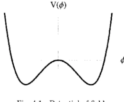
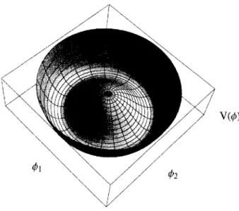
Since the derivatives can only be quadratic, the general form of covariant Lagrangian for a scalar field has the form

(2.109) f(¢) can be put into the metric g~v when we use the curved spacetime for-malism, which we will discuss in detail in the section on the curved space-time. U(¢) is generally divided into the mass term ~m2¢2 and interaction term V(¢).

(2.110) where m is called the mass and V(¢) is the self-interaction. Thus the general form of Lagrangian density in the Minkowski spacetime for a scalar field is given by

(2.111) We have chosen the proper unit of field function such that the first term in Eq. (2.111) has the form without any parameter. We can also put

n

2 in the first term and reformulate the first term as ~2 8~¢8~¢ to make the unit transformation easier, where

n

is called the Planck constant. All the terms in Eq. (2.111) are scalars in the spacetime. Thus the Lagrangian in Eq. ( 2.111) is Lorentz covariant. The corresponding function

9t (

1r, ¢) is given by

(2.112) which does not contain the time derivative terms. We can get the La-grangian density in Eq. (2.111) by inserting Eq. (2.112) into Eq. (2.107) and integrating over 7r using the Gaussian integral formula Eq. (C.21) in

the Appendix C. Thus the generator of time translation corresponding to the Lagrangian Eq. (2.111) is given by

G,

=

j

d3x

[~7T

2

+

~('V¢)

2

+

~m

2

¢

2

+

V(¢)]. (2.113)

2.3.2 Klein-Gordon equation

Now we consider the scalar field as the boson field that

¢

and it satisfy the commutation relations for bosons in Eqs. (2.60) and (2.61). We will

(40)

Quantum Fields 23

show later that we can not construct a consistent formulation for scalar fermions with anti-commutation relations. Calculating the commutator

[¢(x, t), Gt(fr, ¢)] of ¢(x, t) with Gt, we have

[¢(x, t), Gt(fr, ¢)] = ifr. (2.114) Comparing Eq. (2.114) with Eq. (2.81a), we can see that

ao¢

= 1r = -i[¢(x, t), Gt(ir, ¢)]. (2.115) Using commutation relations Eq. (2.81b), we have

fr

= -i[fr(x, t), Gt(fr, ¢)] = (\72- m2)¢(x, t)-V'(¢). (2.116)

In deriving Eq. (2.116), we have used the relation

[fr(x, t), \7' ¢(x', t)]

=

V''[fr(x, t), ¢(x', t)]

=

-i\7' 83(x- x') (2.117) and also an integration by parts. Neglecting the interaction term and com-bining Eqs. (2.115) and (2.116), we find that the field operator for free scalar bosons satisfies the following equation

(2.118) Eq. (2.118) is called the Klein-Gordon equation.

The derivation of the Klein-Gordon equation is based only on the causal-ity principle and the covariance principle. It should be noted that if we use the anti-commutation relations for ¢ and fr, we get [¢(x, t), Gt(fr, ¢)]

=

0.

Gt given by Eq. (2.113) can not be the generator of time translation in this case. Therefore, the Lagrangian Eq. (2.111) can only be used to describe the scalar bosons.1

2.3.3 Solutions of the Klein-Gordon equation

Eq. (2.118) is a wave equation. Thus we have the particle-wave duality for the scalar bosons. We can solve the operator equation (2.118) by expanding

¢(x, t) with respect to a basis. We usually use the set of plane waves up(x) = Npeip·x

for solving the wave equations. Then we have

<f,(x,

t) =

j

d3_{pNpe;p·xap(t),}

(2.119)

(2.120)

1 _{One can also use microcausality to prove that only the boson field can be used in the}

Lagrangian Eq. (2.111) (W. Pauli, Phys. Rev. 58, 716 (1940); M. Fierz, Helv. Phys. Acta 12, 3 (1939)). But here we consider that microcausality is just a result of causality principle. One can prove that the microcausality is satisfied by the scalar boson field with the Lagrangian Eq. (2.111).

(41)

where Np is the normalization constant. Inserting Eq. (2.120) into Eq. (2.118), we get the equation of motion for the operators ap(t):

a(t) = -(p2

+

m2)ap(t). (2.121) The solution of Eq. (2.121) is given by

a (t) = a(l) e-iwpt

+

a(2) eiwpt

p p p ' (2.122)

where a~l) and a~2) are the constant operators in time. Wp is given by the

dispersion relation

(2.123) According to Eq. (2.59a), the field operator¢ is hermitian, ¢t

=

¢. The constraint gives

(2.124) Then the basis expansion Eq. (2.120) becomes

¢(x, t)

=I

d3pNp[a~l)ei(p·X-wpt)

+

a~l)t

e-i(p·x-wpt)]. _(2.125)

Denoting a~1) simply by

aP,

we have

¢(x, t)

=I

d3pNp[apei(p·X-wpt)

+

abe-i(p·X-Wpt)]. _(2.126)

Because fr

=

¢, the basis expansion of the conjugate field is given by 7r(x, t) = -i

I

d 3pNpwp[apei(p·X-wpt)- abe-i(p·x-wpt)J, (2.127) which is consistent with Eq. (2.114).

2.3.4 The commutators for creation and annihilation operators in p-space

The operators

aP

and

at

can be shown to fulfill the commutators for the creation and annihilation operators, i.e.,

(2.128) and

(42)

Quantum Fields 25

The commutation relations Eqs. (2.128) and (2.129) for iip and

at

in the expansion of the field operators can be derived as follows. We introduce

p = ( wp, p) and define the normalized plane waves as

Up(x, t) = Npe-ip·x = 1 e-i(wp·t-p·x) (2.130)

y'2wp(27r)3 _'

where we have used the normalization factor

1

Np = y'2wp(27r)3 ·

Then Eqs. (2.126) and (2.127) become

(/J(x, t)

=

1

d3p[iipup(x, t)

+

abu~(x,

t)],

?T(x, t)

=

-i

1

d3pwp[iipup(x, t) -

abu~(x,

t)].

Projection of the field operator (/J(x, t) on Up and u~ gives

iip =i

I

d

3

xu~(x,t)86¢(x,t)

=(up,¢)

and (2.131) (2.132a) (2.132b) (2.133) (2.134) We have defined the scalar product of two Klein-Gordon wave functions

(h

and ¢2 as

(2.135) where

H

ABo B

=

A(ooB)- (ooA)B. (2.136)

We can easily verify that the plane waves form an orthonormal set with respect to the scalar product Eq. (2.135)

(up', up)

=

i

I

d

3

xu~,

(x, t)

86

up(x, t)

= 83_{(p- p')} _(2.137)

and

(2.138) Similarly,

(43)

Now we evaluate the commutator

[ap, ap,] = i2

1

d3x

1 d

3

x

1

[u~(x,

t)

~

¢(x, t),

u~,

(x1

, t)

~

¢(x 1

, t)]. (2.140)

The functions up ( x, t) are c numbers and commute with the field operators.

We have

[u~(x,

t)

~

¢(x, t),

u~,

(x1 , t)

~

¢(x1, t)] =

u~(x, t)u~,(x

1

,

t)[¢(x, t), ¢(x1 , t)] - u~(x, t)u~,(x1, t)[¢(x, t), ¢(x1 , t)] - u~(x, t)u~,(x1, t)[¢(x, t), ¢(x1 , t)]

+

u~(x, t)u~,(x1_{, t)[¢(x, t),}_¢(x1 , t)]. (2.141)

Using the commutation relations of ¢ and ir, we get

[ap, ap,] = -i

1 d

3

x[u~(x, t)u~,

(x, t) _

u~(x, t)u~,

(x, t)]

=

-i

I

d

3

x[u~(x,t)~u~,(x,t)

=

-(up,u~,)

=

0. (2.142) Similar calculations give

(2.143) Now we calculate the commutator [ap, ab,J· Using the projection formulas Eqs. (2.133) and (2.134), the commutator becomes

[iip,

a~,

I=

-i2

I

d3x

I

d

3

x'[u~(x,

t)

86

J,(x, t), Up' (x', t)

86

J,(x', t)]. (2.144)

According to Eq. (2.136), we have

* HA I HA I [up(x, t) 8o ¢(x, t), Up' (x, t) 8o ¢(x, t)j * I ;_ ;_ I

=

up(x,t)up'(x ,t)[¢(x,t),¢(x ,t)] - u~(x, t)up' (x1 , t)[¢(x, t), ¢(x1, t)] . * I A ;_ I - up(x, t)up'(x, t)[¢(x, t), ¢(x, t)]

+

u~(x, t)up'(x1 , t)[¢(x, t), ¢(x 1 , t)]. (2.145)

Using the commutation relations of¢ and fr, we obtain

[ap, ab,J

=

i

I

d

3

x[u~(x,

t)

~Up'

(x, t)

=

(Up, Up')

=

83(p-p1). (2.146)

Thus we get all the commutators for creation operator

at

and annihilation operator ap.

(44)

Quantum Fields

2.3.5 The homogeneity of spacetime

2.3.5.1 Noether current

27

Now we use the symmetry principle that demands the homogeneity of space-time. The action should possess the symmetry of spacetime translation. We transform the field via ¢(x) ---+ ¢(x- a), where av is a constant four-vector. For an infinitesimal translation 8av, ¢(x) ---+ ¢(x)-8av8v¢(x), we have 8¢(x) = -8av8v¢(x). If we make an infinitesimal change ¢(x) ---+

¢(x)

+

8¢(x) in the field function, we have .C(x) ---+ .C(x)

+

8£(x), where 8£(x) is given by the chain rule,

8£(x) 8£(x)

8(£(x))

=

8¢(x) 8¢(x) + 8(81t¢(x)) alt8¢(x). (2.147)

Taking 8/ 8¢(x) as a functional derivative, we have

8S

j

₄ 8£(y) 8£(x) 8£(x)

8¢(x)

=

d y 8¢(x)

=

8¢(x) - 8

~t

8(81t¢(x)). (2.148) We use the above equation to make the replacement

8£(x) 8£(x) 8S

8¢(x) ---+ 8

~t

8(81t¢(x))

+

8¢(x) (2.149)

in Eq. (2.147). Then we obtain

[

8£(x) _

l

8S

8£(x)

=

alt 8(81t¢(x)) o¢(x)

+ 8¢(x) 8¢(x).

(2.150)

When we transform the fields with an infinitesimal spacetime transla-tion 8av, we have .C(x)---+ .C(x-8a), and then 8(£(x))

=

-8av8v(.C(x))

=

-8v(8av .C(x)). Combining with the first term on the right side of Eq. (2.150), we find

o!fx) 01J(x) = -8M [

8(~~~~~))

( -Ja" 8v1J(x)) +JaM L(x)

l·

(2.151) We introduce the Noether current for the energy-momentum

j~(x)

==

8 (~~~~~))

(Ja" 8v1J(x)) -

Oa~

L(x) =

Oa"B~(x)

(2.152)

with

(2.153) 8~(x) is called the energy-momentum tensor. Then Eq. (2.151) becomes

(45)

2.3.5.2 Conservation of energy-momentum

The action should possess the symmetry of spacetime translation. Under an infinitesimal spacetime translation, the variation of the action should be zero. We have 6S = 0. Then from Eq. (2.154), we have the conservation

of energy-momentum

af.Le~(x)

=

o. (2.155)

Eq. (2.155) is the Noether's theorem for the case of the symmetry of space-time translation.

Now we look at the physical meaning of 8~. We define

(2.156) as the energy-momentum vector.

ez

is called the Poynting vector. Using Eq. (2.153), we have

J

3 [ .C(x) o

l

PJ.L = d x BBo¢(x) 8J.L¢(x)- TJwC(x) . (2.157)

Expressing Eq. (2.155) in terms of the time and space components, Eq. (2.155) becomes

aee(x) \7 ·8i

-at

+

~ 1 / -

o.

Using Gauss's theorem, we have

dPv

dt=O.

Thus Pv is the conserved four-vector. 2.3.5.3 Hamiltonian operator

(2.158)

(2.159)

For the scalar bosons, inserting the Lagrangian density in Eq. (2.111) into Eq. (2.157), we have

Po=

j

d3x

[~(iio¢)

2

+

~(V'¢)

2

+

~m

2

¢

2

+

V(¢)]. (2.160)

Po is defined as the energy of the field ¢ and is also called the Hamiltonian of the field. When we replace the field function ¢ with the field operator

¢,

we call the corresponding operator as Hamiltonian operator.

(46)

Quantum Fields

2.3.5.4 Heisenberg's equations of motion Replacing 80(/J in Eq. (2.161) with ir, we have

Gt

=

fi.

29

(2.162) Therefore the generator of time translation

Gt

is equal to the Hamiltonian operator fi. Replacing

Gt

with fi in Eq. (2.81), we have

iat¢

=

[¢,

fiJ, i8tir = [ir,

fi].

Eq. (2.163) is called Heisenberg's equations of motion. According to Eq. (2.159), we have

[Po, Gt]

=

o.

We can see that Eq. (2.162) is consistent with Eq. (2.159). 2.3.5.5 Hamiltonian operator of free scalar bosons

(2.163a) (2.163b)

(2.164)

We can express the Hamiltonian of free scalar bosons in terms of the cre-ation and annihilcre-ation operators

ab

and

aP.

Inserting the expansion formula for the field operators

¢

and ir, we have

fi

=~I

d3x [ir2

+

("v¢)2

+

m2¢2]

(2.165) The integration over x can be carried out, which gives the delta function.

I

d3

xu;,

(x, t)up(x, t) = -1-83(p- p'), (2.166a)

2wp

I

d3xup'(x, t)up(x, t)

=

2 ~P

e-2iwpt53(p

+

p1). (2.166b)

Using Eq. (2.166), we get

ii

=

~

[-ld3p

w~

(a

a

e-2iwpt-

at

a -a

at+ at at

e2iwpt)

2 2w -p P P P P P -p P

p

-I

d3pL(

-a a

e-2iwpt-

at

a -a

at -at at

e2iwpt)

2w -p P P P P P -p P

p

+

l d3_p_m2

_(a

a

_{e- 2iwpt}

_+at

a +a

_{at +at at}

_e2iwpt)J _(2.167)

2w -p P P P P P -p P ·