Heliosheath processes and the structure of the heliopause: modeling energetic particles, cosmic rays, and magnetic fields

HAL Id: insu-01421103

https://hal-insu.archives-ouvertes.fr/insu-01421103

HAL is a multi-disciplinary open access archive for the deposit and dissemination of sci-entific research documents, whether they are pub-lished or not. The documents may come from teaching and research institutions in France or abroad, or from public or private research centers.

L’archive ouverte pluridisciplinaire HAL, est destinée au dépôt et à la diffusion de documents scientifiques de niveau recherche, publiés ou non, émanant des établissements d’enseignement et de recherche français ou étrangers, des laboratoires publics ou privés.

Heliosheath processes and the structure of the

heliopause: modeling energetic particles, cosmic rays,

and magnetic fields

Nikolai V. Pogorelov, Horst Fichtner, Andrzej Czechowski, Alexandre

Lazarian, Bertrand Lembège, J. A. Le Roux, M. S. Potgieter, K. Scherer, E.

C. Stone, R. D. Strauss, et al.

To cite this version:

Nikolai V. Pogorelov, Horst Fichtner, Andrzej Czechowski, Alexandre Lazarian, Bertrand Lembège, et al.. Heliosheath processes and the structure of the heliopause: modeling energetic particles, cos-mic rays, and magnetic fields. Space Science Reviews, Springer Verlag, 2017, 212 (1-2), pp.193-248. �10.1007/s11214-017-0354-8�. �insu-01421103�

arXiv:1612.02339v1 [physics.space-ph] 7 Dec 2016

Heliosheath Processes and the Structure of the Heliopause: Modeling Energetic Particles, Cosmic Rays, and Magnetic Fields1

N. V. Pogorelov,1 H. Fichtner,2 A. Czechowski,3 A. Lazarian,4 B. Lembege,5 J. A. le Roux,1 M. S. Potgieter,6 K. Scherer,2 E. C. Stone,7R. D. Strauss,6 T. Wiengarten,2 P. Wurz,8 G. P. Zank,1 M. Zhang9

1 _{Department of Space Science, University of Alabama in Huntsville, AL 35805, USA} 2

Institut f¨ur Theoretische Physik IV, Ruhr-Universit¨at Bochum, 44780 Bochum, Germany

3

Space Research Centre, Warsaw, Poland

4_{University of Wisconsin, Madison, USA} 5

Laboratoire Atmosph`eres, Milieux, Observations Spatiales (LATMOS), Guyancourt, France

6

North-West University, Campus Potchefstroom, South Africa

7_{California Institute of Technology, Pasadena, USA} 8

Universit¨at Bern, Switzerland

9

Florida Institute of Technology, Melbourne, USA

Abstract

This paper summarizes the results obtained by the team “Heliosheath Processes and the Structure of the Heliopause: Modeling Energetic Particles, Cosmic Rays, and Magnetic Fields” supported by the International Space Science Institute (ISSI) in Bern, Switzerland. We fo-cus on the physical processes occurring in the outer heliosphere, especially at its boundary called the heliopause, and in the local interstellar medium. The importance of magnetic field, charge exchange between neutral atoms and ions, and solar cycle on the heliopause topology and observed heliocentric distances to different heliospheric discontinuities are discussed. It is shown that time-dependent, data-driven boundary conditions are necessary to describe the heliospheric asymmetries detected by the Voyager spacecraft. We also discuss the structure of the heliopause, especially due to its instability and magnetic reconnection. It is demon-strated that the Rayleigh–Taylor instability of the nose of the heliopause creates consecutive layers of the interstellar and heliospheric plasma which are magnetically connected to different sources. This may be a possible explanation of abrupt changes in the galactic and anomalous cosmic ray fluxes observed by Voyager 1 when it was crossing the heliopause structure for a period of about one month in the summer of 2012. This paper also discusses the plausibil-ity of fitting simulation results to a number of observational data sets obtained by in situ and remote measurements. The distribution of magnetic field in the vicinity of the heliopause is discussed in the context of Voyager measurements. It is argued that a classical heliospheric current sheet formed due to the Sun’s rotation is not observed by in situ measurements and should not be expected to exist in numerical simulations extending to the boundary of the he-liosphere. Furthermore, we discuss the transport of energetic particles in the inner and outer heliosheath, concentrating on the anisotropic spatial diffusion diffusion tensor and the pitch-angle dependence of perpendicular diffusion and demonstrate that the latter can explain the observed pitch-angle anisotropies of both the anomalous and galactic cosmic rays in the outer heliosheath.

1

Introduction

The Sun and the local interstellar medium (LISM) move with respect to each other creating an interaction pattern likely similar to many other stellar wind collisions with their local interstellar environments. One would expect differences in details though. E.g., jets and collimated outflows are ubiquitous in astrophysics, appearing in environments as different as young stellar objects, accreting and isolated neutron stars, stellar mass black holes, and in supermassive black holes at the centers of Active Galactic Nuclei. Despite the very different length scales, velocities and composition of these various types of jets, they share many basic physical principles. They are typically long-duration, supersonically ejected streams that propagate through and interact with the surrounding medium, exhibiting dynamical behavior on all scales, from the size of the source to the longest scales observed. Charged particle flows emitted by stars moving through the in-terstellar space form astrotails which can be very different in shape and length, depending on the astrophysical object under consideration. The Guitar Nebula is a spectacular example of an Hα

bow shock nebula observed by the Hubble Space Telescope (HST) and Chandra [1]. The physics of the interaction is very similar to that of the solar wind (SW)–LISM interaction, but there are substantial differences in the stellar wind confinement topology. Mira’s astrotail observed by the Galaxy Evolution Explorer [2] extends to 800,000 AU. Carbon Star IRC+10216, on the contrary, exhibits a very wide astropause and a short astrotail [3]. The heliotail cannot be observed from out-side, but its signatures have been identified in energetic neutral atom (ENA) measurements with the Interstellar Boundary Explorer (IBEX) [4]. The heliotail properties have been investigated theoretically [5] and numerically [6, 7, 8].

The goal of this paper is to demonstrate that a better knowledge of the SW and LISM properties makes it possible to explain, at least qualitatively, a number of observational data. Moreover, it is clearly understood now that proper interpretation of observations is impossible without taking into account genuine time dependence of the SW–LISM interaction. To reproduce in situ and remote observations of the distant SW, we need to take advantage of the full set of observational data in the inner heliosphere. On the other hand, in situ measurements by Voyager 1 (V1 and remote observations of ENA fluxes from IBEX, Lyα backscattered emission from the Solar Heliospheric

Observatories (SOHO) Solar Wind Anisotropy (SWAN) experiment, Lyα absorption profiles in

the directions toward nearby stars from the Hubble Space Telescope (HST), 1–10 TeV cosmic ray anisotropy from multiple air shower missions (a number references can be found in [9]), and starlight polarization from [10] provide us with invaluable information about the LISM properties. The availability of realistic, data driven boundary conditions, makes SW–LISM interaction models a powerful tool to investigate the properties of the heliospheric interface.

It is not the purpose of this paper to provide an extensive review of the community efforts to investigate the physical processes in the vicinity of the heliospheric interface, for those see, e.g., the reviews [11], [12], [13], or [14]. This is rather a report on the activity of an international team with a name coinciding with the paper title that was recently supported by the International Space Science Institute (ISSI) in Bern, Switzerland. For this reason, we mostly address scientific results obtained by the team itself and their relation to other recent studies. We also identify the challenges that emerged in the investigation of the structure of the heliopause (HP) and heliosheath processes, especially related to energetic particles, cosmic rays, and magnetic fields. In this paper we also address a number of issues discussed in the review article [15].

2

Constraints on the model boundary conditions from

obser-vations

From a purely magetohydrodynamic (MHD) perspective, the global structure of the SW–LISM interaction is clear. When two plasma streams collide, a tangential discontinuity (here the HP) should form that separates the SW and LISM plasmas. This discontinuity can be interpreted as a constituent component of the solution to an MHD Riemann problem [16]. Other MHD disconti-nuities (fast and slow shocks, contact and rotational (Alfv´en) discontidisconti-nuities, slow- and fast-mode rarefaction waves) may or may not form on the LISM and SW sides of the HP, but the presence of a tangential discontinuity is obligatory. The SW–LISM boundary cannot be a rotational disconti-nuity, as suggested in [17], because this means the absence of any separation boundary. Moreover, the SW and LISM velocities at any point on the HP would be in the same direction and have the magnitudes equal to the Alfv´en speed on both sides. Early studies of the SW–LISM interaction were mostly theoretical because no boundary conditions were available either in the SW or the LISM. The seminal paper [18] proposed a powerful tool to solve the SW–LISM interaction prob-lem through the application of the MHD equations. The possibility to use continuum equations to model the collisionless SW is supported by the dramatic decrease in the ion mean free path due to scattering on magnetic field fluctuations caused by numerous kinetic instabilities typical of the SW flow. Although it is known that only the global, macroscopic structure of the plasma flow can be described using a continuum description, the efficiency of the MHD/hydrodynamic approach cannot be overestimated.

The importance of charge exchange between the LISM hydrogen (H) atoms and SW ions has been known since late 60’s [19, 20, 21, 22, 23]. The resonant charge exchange between ions and neutral atoms which have non-zero relative velocity is a death/birth process in which a parent ion-atom pair disappears producing an ion with the parent neutral ion-atom properties and an ion-atom with the properties of the parent ion. Newly created (secondary) atoms continue to move unaffected by the electromagnetic field, whereas newly born (pickup) ions (PUIs) are acted upon the motional electric field until their velocity becomes equal to the velocity of the background plasma [18]. The PUI distribution function is originally a ring-beam, but they quickly scatter onto a shell distribu-tion. With increasing the heliocentric distance, some particles fill in the shell at lower energies, while other particles are accelerated to higher energies [24], so PUIs are not in equilibrium with the SW protons. Secondary neutral atoms can propagate far into the LISM where they may ex-perience charge exchange producing a new population of PUIs, which arguably produce so-called energetic neutral atoms (ENAs) measured by the Interstellar Boundary Explorer (IBEX) [25, 26]. A number of important consequences of such charge exchange had been identified long before the first numerical simulation was made. These are the SW deceleration and heating, and filtration of interstellar atoms at the HP, which prevents a substantial fraction of those atoms from entering the heliosphere and results in a so-called hydrogen wall in front of the HP, and many others. More-over, charge exchange decreases asymmetries of the three-dimensional (3D) heliosphere caused by the action of the interstellar magnetic field [27]. This raises questions about the coupling of the heliospheric magnetic field (HMF) and ISMF at the HP.

Voyager 1 (V1) crossed the HP in August 2012 [28, 29, 30, 31], whereas Voyager 2 (V2) is

still in the inner heliosheath – the SW region between the HP and the heliospheric termination shock (TS). The spacecraft crossings of the TS and HP, and measurements performed in their

vicinity were accompanied by a number of interesting physical phenomena, which will be ad-dressed in this paper in some detail: (1) the asymmetry of the heliosphere and the contribution of time-dependent factors; (2) the heliospheric current sheet (HCS) behavior; (3) anisotropy in the anomalous and galactic cosmic ray (ACR and GCR) fluxes; (4) a prolonged, almost two-year period of sunward flow at V1 before it crossed the HP; (5) puzzling variations in the ACR and GCR flux within a month while V1 was crossing a finely structured HP; (6) observations of the LISM turbulence spectrum and issues related to the production of an enhanced flux of energetic neutral atoms (ENAs) originating beyond the HP and propagating toward IBEX detectors from directions roughly perpendicular to magnetic field lines draped around the HP [25]; (7) the nature of the ISMF draping and the change of the ISMF direction as the LISM flow approaches the HP; (8) the HP instability and possible signatures of magnetic reconnection in its vicinity; (9) the ratio between the parallel and perpendicular diffusion coefficients that can be derived from V1 observa-tions, etc. We will also discuss our predictions regarding the inner heliosheath width in the V1 and

V2 directions. Finally, the flow in the heliotail will be discussed together with its possible effect

on the anisotropy of the multi-TeV GCR flux observed in a number of air shower experiments.

3

What is the proper definition of the heliopause and where is

it located?

When two plasma streams collide, a tangential discontinuity is formed at the collision interface provided that dissipative and finite conductivity effects are absent, i.e., when an ideal MHD ap-proximation is applicable. In the context of the SW–LISM interaction, this tangential discontinuity is called the HP [32]. The HP separates the LISM and SW flows. The boundary conditions in the HP frame are formulated as follows: (i) the sum of the thermal and magnetic pressures across the HP is continuous and (ii) the velocity and magnetic field vectors are tangent to the HP surface. All other quantities may experience arbitrary jumps. The structure crossed by V1 cannot be a rotational discontinuity because rotational discontinuities are permeable, which means that either the SW or LISM plasma is crossing the surface of this discontinuity at the Alfv´en velocity. Furthermore, and that there should be a real HP somewhere ahead. In ideal MHD, a tangential discontinuity cannot degenerate into a rotational discontinuity, except for a trivial case with equal densities on both sides of the HP, because they belong to different classes [33]. The possibility of mixing of the SW and LISM plasmas in the vicinity of the HP, i.e., its dissipative/resitive structure, has been summarized in [34], where it was shown that even anomalous resistivity would likely result in a structure of about 0.01 AU width. This is 30 times narrower than the structure that was crossed by V1 within a month.

The applicability of the ideal MHD equations to model the SW–LISM interaction is not obvi-ous. It is mostly based on the assumption that the ion distribution function is isotropic away from discontinuities. Of major concern is the presence of a nonthermal ion component, namely PUIs, both in the SW and LISM [35]. Most numerical simulations so far have been based on the one-ion-fluid approach where all ions are treated as a thermal mixture. PUIs are created wherever charge exchange occurs, but they are not distinguished from the original thermal population of ions. The momentum and energy of thermal ions and PUIs are summed up. This approach is different from multi-ion approaches, e.g. [36], where several populations of PUIs were introduced depending on

the region where they are created and the population of neutral hydrogen atoms that participates on each charge-exchange process. More precisely, they used 10 populations of neutral atoms and four types of ions. Regardless of the axisymmetric statement of the problem, the results of [36] are of fundamental importance for our understanding of physical processes in the heliosheath and near the HP because they demonstrate the kinetic behavior of PUIs throughout the heliosphere. Additionally, it was proved by direct numerical simulations in [36] that charge exchange between PUIs and hydrogen atoms in the inner heliosheath results in a considerable momentum and energy removal from plasma to ENAs. As a consequence, the TS moves farther from the Sun, while the heliocentric distance of the HP decreases. This makes the inner heliosheath thinner, in accordance with V1 observations (see also 3D, multi-fluid simulations in [37]). On the other hand, it is shown in [38] that the effect of PUIs may be overestimated if the charge exchange cross-section is as-sumed constant while calculating the collisional integral – an approach used in [39, 40] and similar to it. This is especially true if the plasma distribution function is not Maxwellian (e.g., Lorentzian (kappa) distribution). In particular, the charge exchange source term diverges for κ < 2 if the

cross-section dependence on energy is ignored. The IHS width can also be decreased by thermal conductivity [41]. It was shown [36] that the presence of PUIs does not affect the flow near the HP in a topologically dramatic fashion. Theoretical analysis preformed in [42] and [17] suggests that ACRs may be of dynamic importance, possibly creating additional separation surfaces inside the HP. No simulation results have been obtained so far to support or disprove that theory.

While the thickness of the inner heliosheath can be decreased by treating PUIs a separate entity, the heliopause can also exhibit inward excursions due to the HP instability. The latter does not necessarily result in the decrease of the heliosheath width. In fact, there are no observations that would tell us where the TS is now.

Following prior investigations [43, 44, 45, 40, 46, 47, 48], the problem of the HP stability was revisited by 3D simulations [49] based on a more realistic distribution of the ISMF draping around the HP (see also an analytical study [50], where it was shown that there are always perturbations that grow at the linear stage). In summary, the HP is not a classical MHD discontinuity, but is subject to both Rayleigh–Taylor-like and Kelvin–Helmholtz-like instabilities caused by charge exchange and shear flows near the HP. According to [46], the mechanism of the Rayleigh–Taylor instability in this case is due to the momentum and energy exchange between protons and neutral atoms. It has been shown in [49, 51] that such instability may form complicated structures where regions of the SW and LISM plasma follow each other (see Fig. 1). Similar structures may also be produced by magnetic flux transfer events described in [52]. According to [48], the time evolution of the HP instability has no single frequency provided that both primary and secondary neutral atoms are taken into account. In 3D simulations performed in the presence of both HMF and ISMF, deep LISM plasma protrusions related to the HP instability appear at least once per two solar cycles. Their evolution, however, is longer. As mentioned in [49], the Rayleigh–Taylor instability develops more efficiently when the HMF strength decreases. This situation is typical for the HP when the SW in its vicinity carries a sectored region of alternating HMF polarity, which are subject to magnetic reconnection and turbulence leading to the magnetic field dissipation. Once a protrusion occurred, it further develops being shaped by the HMF. As a result of instability, we observe plasma regions that are magnetically connected either to the LISM or the SW. If cosmic ray diffusion perpendicular to magnetic field lines is small compared with the parallel diffusion, consecutive decreases and increases in the GCR flux should be observed. The fluxes of termination shock ions (ACRs) will have maxima in the interface regions where GCRs have minima. More

Figure 1: Instability of the HP. Clockwise, the distributions ofBy,|B|, plasma number density, and

pressure f the magnetic field and its magnitude in the SW–LISM interaction with the solar cycle taken into account.

detailed simulations of GCR and ACR fluxes are necessary to support this idea.

4

What is the correlation between the IBEX, SOHO, and

Voy-ager observations?

Remote sensing observations using ENAs are complementary to in situ observations by the Voy-ager spacecraft. ENAs are created by charge exchange between neutral atoms and ions in the heliosheath, whereby the momentum exchange is minimal. Thus, the created ENAs keep the ve-locity and direction of the original ion, but are freed from the electromagnetic forces and therefore follow ballistic trajectories. Thus, ENAs can be used for remote sensing of plasma populations in

space [53]. These observations can be done from the Earth orbit and make it possible to investigate the entire sky. However, ENA observations are always line-of-sight observations and therefore have to be interpreted by theory and modeling for a full understanding.

The first ENA observation of the heliosheath were performed with the HSTOF sensor of the CELIAS instrument on the SOHO mission for hydrogen ENAs in the energy range from 55–80 keV [54]. In [55], the final analysis of these data is presented for hydrogen and helium ENAs originat-ing in the heliosheath. At lower energies, in the range from 400 eV to 5 keV, the first hydrogen observations were done by the ASPERA-3 and ASPERA-4 ENA instruments on the Mars Express and Venus Express spacecraft [56]. In [57], the final analysis of these data is presented, which is in agreement with the IBEX data. ENA energy spectra were compiled already from those first data sets. By considering the charge exchange cross-sections, the energy spectra of protons in the heliosheath were derived, extending the range covered by the instrumentation of the Voyager spacecraft. Before IBEX measurements, the covered energy range spanned from 400 eV to 80 keV [56, 58, 55, 59], including the HENA data from the IMAGE mission, with the most recent com-pilation of the ENA energy spectra given in [57]. From the fit of the proton spectra, which were derived from these ENA energy spectra, to the in situ proton spectra from Voyager at higher ener-gies, which is the only fit parameter, the thickness of the heliosheath in the upwind direction can be estimated to be between 35–70 AU.

The IBEX mission [60] is the first space mission dedicated solely to the investigation of the heliospheric interface with the interstellar medium. IBEX performs full-sky observation of ENAs with two ENA cameras, IBEX-Lo [61] and IBEX-Hi [62], combined covering the energy range from 10 eV to 6 keV. The ENA signal recorded by IBEX has its origin in the plasma populations beyond the heliospheric termination shock at distance of more than 100 AU from the Sun, which are explored by the Voyager spacecraft at the same time. IBEX full-sky ENA measurements to-gether with Voyager in situ plasma measurements allowed the space science community to make a major step forward in the scientific investigation of the heliospheric interface.

The first, and completely unexpected, discovery of IBEX was the ENA ribbon signal [25, 63], which is a narrow band in the ENA sky maps, about 20◦–40◦ wide, of enhanced ENA fluxes, initially observed over the energy range from 0.7 to 2.7 keV (see Fig. 2). The ribbon is best seen in the energy range between 0.5 keV and 4.7 keV [64]. The ENA ribbon is a stable signal that has been observed in every IBEX map recorded since 2009 in the IBEX-Hi images [64]. The fluxes in the ENA ribbon are up to about 2–3 times larger than the surrounding ENA fluxes, the globally distributed ENA fluxes, with the ribbon fluxes peaking around 0.7 keV, which corresponds to a flow velocity of 350 km/s (left panel of Fig. 2). At higher energies above 2 keV the ribbon starts to become more fragmented and the ribbon structure at energies of 4.7 keV and above is difficult to identify. By significantly improving the identification and removal of the background in the

IBEX-Lo ENA images this ribbon could be identified down to energies of 100 eV, also finding at

the lowest energies increasing spatial fragmentation [65].

The origin of the ribbon is still debated. From comparisons between the outer heliosheath and ribbon models, it was surmised already at the time of the ribbon discovery that ISMF in the outer heliosheath is roughly perpendicular to the directions toward the IBEX ribbon, that is where

~

B ·~r = 0, where ~r is the radial line-of-sight (LOS) direction and ~B is the interstellar magnetic field

[25, 64]. Unfortunately, both Voyager trajectories do not overlap with the ENA ribbon (see Fig. 2), so no in situ data are available for these parts of the sky to assist the interpretation of the ENA observations. The proposed location of origin of the ribbon ENAs ranges from the heliospheric

Figure 2: Left panel: ENA energy spectra for three different regions in sky as indicated by coor-dinates in the inset [57]. Blue symbols: boundary of the low ENA intensity region, red symbols: ribbon region in the ecliptic, black symbols: region in the southern hemisphere. The orange dashed line indicates the upper limit on heliospheric ENAs derived from Lyα observations. Crosses

in-dicate IBEX-Lo, circles inin-dicate IBEX-Hi observations. Right panel: Full sky map for ENAs at 1.1 keV from IBEX-Hi with the directions of the two Voyager spacecraft and the upwind direction (nose) indicated [64].

termination shock, the inner and outer heliosheath, all the way to the nearby edge of the local interstellar cloud [25, 26, 66, 67, 68, 69, 70, 71]. All models involve charge exchange between ions and neutral atoms. Alternatively, a density fluctuation in the neutral interstellar gas passing over the heliosphere has been proposed, which would cause a localized increase of the charge exchange, thus locally increasing the production of the globally distributed ENA flux [72].

The energy distribution of ions is one of the important quantities for every plasma population, because it affects the definition of boundaries between different plasma populations. Thus, de-riving the energy spectra in the heliosheath from the ENA observations is an important science objective. First analyses of IBEX ENA data covered the energy range down to 100 eV [73, 65], where the observed spectral shape are power laws with indices ofγ = −1.4 ± 0.1 for all sky

direc-tions. Because the observed energy spectra are power laws with negative exponents (see Fig. 2 for example), the lowest energies contribute the most to the pressure, and when the energies down to 100 eV are considered the pressure is already dominated by the lowest energy measured. In [64], full sky maps of the LOS-integrated-pressure from the measurements of the globally distributed ENA flux were derived, peaking in the nose direction at about 40 pdyn AU cm−2 for the energy range from 0.2 to 4.7 keV (where 1 pdyn AU cm−2= 0.015 N m−1).

In the latest IBEX analysis of the IBEX-Lo data, the identification and removal of background sources was significantly improved and the ENA energy range could be extended down to almost 10 eV for selected locations in the sky [74], as shown in Fig. 3. It was found that the power law shape of the ENA energy spectrum continues to the lowest energies accessible to IBEX-Lo, for some directions in the sky, with a with slope ofγ = −1.2 ± 0.1 for most of the sky directions.

However, there is a roll-over of the ENA energy spectrum at the downwind hemisphere. This has important consequences for the pressure balance in the heliosheath: for the downwind hemisphere the LOS-integrated-pressure is 304 pdyn AU cm−2 and for the V1 region it is 66 pdyn AU cm−2.

Figure 3: Energy spectra of heliospheric ENAs in the downwind hemisphere. Black symbols are data from [74], red triangles down from [65], and orange triangles up are from [73] for similar regions in the sky. The black line shows the power law with slope γ = −1.1, which describes

the energy spectra at energies above 0.1 keV well. For lower energies, the earlier energy spectrum [74] was consistent with a uniform power law continuing to the lowest energies (red dashed line); the newest study shows that the energy spectrum rolls over and the signal vanishes at low energies (black dashed-dotted line).

Moreover, from this measurement the “cooling thickness” of the heliosheath at the downwind side of 220±110 AU could be derived assuming pressure balance across the termination shock, while

the heliosheath thickness in the V1 direction is 50 AU. The term of “cooling length” was introduced in [64] to emphasize that ENAs of any particular energy should have a maximum line-of-sight integration length. ENAs born beyond this length cannot return to IBEX.

5

Plasma and magnetic field modeling in the context of

obser-vational data

5.1

Interplay between charge exchange,

ISMF draping,

and

time-dependence

Charge exchange of the LISM neutral atoms with both LISM ions decelerated by the HP and SW ions makes the heliosphere more symmetric (see Fig. 4). The reason of this is simple. Since the unperturbed ISMF vector, B∞, is directed to the southern hemisphere at an angle of 45◦ to the

LISM velocity vector, V∞, which is directed from the right to the left in the figure, the magnetic

pressure rotates the HP clockwise. This rotation exposes the northern side of the HP to the LISM plasma shifting the LISM stagnation point and the corresponding maximum of the plasma number density northward. As a result, more charge exchange occurs in that region creating more ions with the velocity of the parent neutral atoms, which should be decelerated by the HP and exert additional thermal pressure on the HP rotating it counterclockwise. In summary, while the ISMF tends to make the heliosphere asymmetric, charge exchange, on the contrary, symmetrizes it. For this reason, a squashed shape TS in the left panel of Fig. 4 disappears when charge exchange

Figure 4: Plasma temperature distributions in the meridional plane for the ISMF vector, ~B∞,

belonging to this plane with a tilt of 45◦ to the LISM velocity vector, ~B∞, andB∞ = 2.5 µG:

(a) the ideal MHD calculation without an IMF; (b) the plasma-neutral (two-fluid) model with

nH∞ = 0.15 cm−3. The straight lines in the northern and southern hemispheres correspond to the

V1 and V2 trajectories, respectively. The TS asymmetry is considerably smaller in case (b) due to the symmetrizing effect of charge exchange. [From [27] with permission of the AAS.]

is taken into account, as seen from the right panel of Fig. 4. Thus, the difference of 10 AU in heliocentric distances at which V1 and V2 crossed the TS can easily be explained by the action of the ISMF draped around the HP [75, 76, 77, 78, 79, 8] if charge exchange is ignored, but it becomes very small once charge exchange is taken into account [27].

If charge exchange symmetrizes the heliosphere in general and the TS, in particular, the ques-tion arises about the reason of the observed difference. The TS is responding to changes in the ratio between the SW and LISM ram pressures (ρV2

R/ρ∞V∞2). Ulysses measurements [80]

iden-tified the presence of slow wind at low latitudes and fast wind at high latitudes. The boundary between slow and fast winds is a function of solar cycle: the latitudinal extent of the slow wind is the smallest at solar minima and it can be as large as90◦_{(no direct measurements have ever been}

done at latitudes well above 80◦_{) at solar maxima. In [81], the SW ram pressure is assumed to}

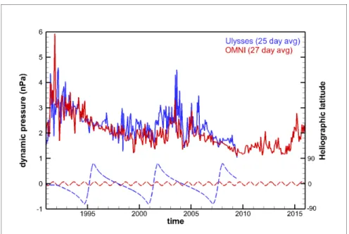
be same in the slow and fast SW. Indeed, a comparison of Ulysses and OMNI data made in [82] resulted in the conclusion that those are in quantitative agreement. We reproduce observational data from Ulysses and OMNI in Fig. 5 on linear scale as functions of time. In addition to the ram pressure, we also show the Ulysses and Earth latitudes. Clearly there are deviations between observational data at non-coinciding latitudes, some of them should likely be attributed to such transient phenomena as coronal mass ejections and corotating interaction regions. However, such deviations are important once we are interested in realistic boundary conditions for SW–LISM simulations. Another, possibly better, “latitudinal invariant” was considered in [83]. This is the SW energy fluxW . However, although the average W is very close at Ulysses and OMNI, there

Figure 5: Time evolution of the SW ram pressure at Ulysses and OMNI is shown together with the spacecraft latitudes as functions of time. [Data courtesy of the SPDF COHOWeb database.]

Ulysses data analysis in [84, 85], the ram pressure in the genuine slow wind (not only the veloc-ity magnitude but also the SW composition was taken into account to discriminate between the fast and slow winds) was ∼ 0.8 of that in the genuine fast wind during solar cycle 22 (SC22),

but became ∼ 1.1 during solar cycle 23 (SC23). Notice that the slow wind ram pressure became

larger than that in the fast wind during SC23. The ram pressure of the slow wind decreased by

∼ 12% between SC22 and SC23, while the decrease in the fast wind was ∼ 37%. As seen from

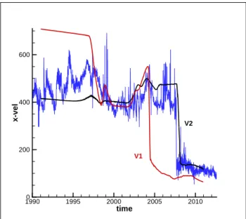
Fig. 6, the simulation that takes into account this effect reproduces both the time and distance at which Voyagers crossed the TS [85]. This shows that time-dependence effects are important for the explanation of the observed asymmetry of the heliosphere. On the other hand, the HP in that simulation, which was performed only for the period of time when the boundary conditions from

Ulysses measurements were available, decreased its heliocentric distance in the V1 direction only

by ∼ 2 AU and ultimately reached distance of ∼ 140 AU in 2010. The heliosphere was clearly

decreasing in size at the end of simulation and it is possible that it continued decreasing in response to the decrease in the SW ram pressure to the value of 122 AU, when the HP was crossed by V1. On the other hand, the simulations in [86], where V2 observations were extended in a spherically symmetric manner over a moving spherical boundary with the radius equal to the V2 heliocentric distance, show considerably larger excursions of the HP. A possible reason for this may be that the plasma quantities oscillate in unison over the inner boundary with the amplitude of spacecraft observations. The Ulysses-based solar cycle simulations in [85] show that the HP motion is mostly determined by the differences between solar cycles rather than by the changes on the latitudinal extent of the slow wind.

The HP motion closer toward the Sun also results in negative values of the SW radial velocity component,VR, near the HP. A question is about how large those components can be. The radial

velocities that were derived from V1 LECP data in the inner heliosheath [88, 89] are smaller than the value of approximately−40 km/s which may have resulted from a HP shift from 140 AU to

time x -v e l 19900 1995 2000 2005 2010 200 400 600 V2 V1

Figure 6: The distribution of the radial component of the plasma velocity vector along the V2 (black line) and V1 (red line) trajectories. Voyager 2 observations are shown with the blue lines. [From [85] with permission of the AAS.]

122 AU in 2 years. Another possibility has been proposed in [87]. As seen in Fig. 7, which shows the space-time plots of the plasma number density and magnetic field magnitude in a direction imitating the V1 trajectory, such behavior of the SW velocity is typical if the solar cycle is taken into account (see also, e.g., [90]). It is also possible that V1 may cross a LISM region with positive

vR. The latter regions extend into the LISM as far as 50 AU. In the inner heliosheath, the regions

of negativeVR are smaller (∼ 7 AU). The existence of both regions had been predicted in [91],

two years before they were measured by V1. Magnetic barriers are created due to the interaction of slow and fast streams in the SW (see, e.g., [92]). However, only in [91, 87] was it noticed that SW streamlines that start near the equatorial plane become occasionally concentrated between a magnetic barrier and the HP. Since such a barrier has finite latitudinal extent, those streamlines diverge towards the Sun when the barrier disappears. This is seen in Fig. 8.

An additional conclusion of [87] is that V2, because of solar cycle parameters, is unlikely to see backward SW flow if it was observed by V1. The reasons are as follows: (1) its velocity is less than V1 and (2) it crossed the TS later, within a solar cycle, than V1. As a result, the V2 trajectory should miss the region of substantial negative velocity. Another interesting consequence is that V1 may ultimately observe positive radial velocity components in the LISM approximately in 2020–2021.

5.2

Magnetic field in the inner heliosheath and beyond

The Voyager magnetic field instrument (MAG) provided us with invaluable distributions of the HMF at V1 and V2. The HMF exhibits turbulent fluctuations on both kinetic and small scales. It is seen from [93, 29] that the variability and especially the number of HMF vector reversals at sector boundaries was much greater before each of the spacecraft crossed the TS. This is puzzling if we assume that the sectors are due to the global heliospheric current sheet (HCS). In this case,

Figure 7: Space-time plots of (left) plasma number density and (right) magnetic field magnitude in a direction imitating the Voyager 1 trajectory. The black curve shows the line wherevR = 0. The

black straight line is a possible trajectory of a spacecraft moving at the V1 velocity. [From [87] with permission of the AAS.]

Figure 8: Magnetic barriers (left panel) and related negative values of the SW radial component (right panel). The streamlines start on a heliocentric circle of 15 AU radius and are shown neglect-ing the out-of-plane velocity component. The TS is shown with a thick black line. Distances are given in AU. They-axis is directed into the figure plane. [From [87] with permission of the AAS.]

the number of sector crossings should gradually increase to very large values while the velocity component normal to the HP tends to zero. We should recall here that the radial velocity com-ponent was zero to negative for about 8 AU before the HP crossing, which makes it doubtful that the existence of the HCS structure is determined entirely by the tilt between the Sun’s rotation and magnetic axes. This pattern can be seen qualitatively in Fig. 9 (the right panel), where the disruption of the HCS structure is due to the tearing mode instability caused by numerical resis-tivity. It is worth noticing that the figure shown in this panel is drastically different from similar figures in [94, 95], although the boundary conditions were chosen to be identical. In particular, in [95] (Figs. 2 and 3), one can see something resembling a radially-oriented discontinuity crossing the IHS. This discontinuity is not related to the boundary between the slow and fast SW, and its presence therefore has no explanation. In contrast to [91, 95], where the heliospheric magnetic field dissipates in the IHS completely, [85] rather observe a chaotic disruption of the HCS, which is a likely fate for it regardless of the actual mechanism, turbulence or magnetic reconnection, responsible for this phenomenon. On the other hand, sector crossings were observed by V1 and are being observed by V2 in the inner heliosheath, although the sector widths are not as small as one would expect. Additionally, numerous sector crossings seem to have been observed when the HMF strength was close to or below the MAG accuracy. Clearly, current sheets can be created not only due to the above-mentioned tilt. This can be due to stream interactions, which are ob-served throughout the heliosphere. Additionally, observations of the magnetic equator of the Sun from the Wilcox Solar Observatory show small-scale non-monotonicity. Any change in the sign of the tilt derivative at the latitudes of Voyager spacecraft creates a current sheet with a sector size considerably greater that those due to the Sun’s rotation. These issues are of importance because they tell us what to expect from the magnetic field distribution as the SW approaches the HP. Is the sector structure of the HMF destroyed by SW turbulence, as shown in [49], while other current sheets still exist and are detected by spacecraft? Answering this question is of importance not only to understand the heliosheath flow, but also the flow in the heliotail [6, 7].

The V1 crossing of the heliospheric boundary was accompanied by a change in the magnetic field [28]. Before the crossing, the magnetic field direction was consistent with the Parker spiral. After the crossing the direction of the field changed, but only by a small amount (∼ 20◦). Since there is no particular reason for the ISMF direction to remain close to that of the HMF, this obser-vation was for some time regarded as an indication that V1 might not yet be in the LISM. However, a similar set of the magnetic field elevation and azimuthal angles in the LISM was reported before the crossing in [91] (see also [49]). On the other hand, numerical simulations in [49] demonstrated (see Fig. 9, left panel) that the elevation angle was greater than the observed value when the LISM properties, especially the direction of the LISM velocity, were taken from [96, 97]. The updated properties of the LISM proposed on the basis of IBEX observations in [98] are in better agreement with V1 observations and, as in [91], make it possible to reproduce the ISMF draping around the heliopause [99].

A simple explanation of the V1 measurements of the draping angles was proposed in [100]. It relies on the fact that the V1 trajectory direction and the direction of the unperturbed ISMF, assuming that the ISMF is directed into the center of the IBEX ribbon [101] have almost the same heliographic latitude (∼ 34.5◦_{). The deviation of the ISMF direction from the ribbon center}

increases with decreasing the ISMF strength [99]. The draped magnetic field line must ultimately become parallel to its unperturbed direction at large distances from the HP. If a magnetic field line passing through V1 has a shape close to a great circle in the projection of the celestial sphere, it

Distance, AU λ δ 50 100 150 90 135 180 225 270 315 -20 0 20 40 λ δ

Figure 9: Left panel) Instantaneous distributions of the B elevation and azimuthal angles (δ and λ). (Right panel) Transition to chaotic behavior in the inner heliosheath. Magnetic field strength

distribution (inµG) is shown in the meridional plane. The angle between the Sun’s rotation and

magnetic axes is30◦_{. [From [49] and [85] with permission of the AAS.]}

may become nearly parallel to the Parker HMF.

Before reaching the heliopause V1 encountered two “precursors,” where the flux of heliospheric energetic particles dropped sharply, although by a smaller amount that at the heliopause, while the magnetic field strength sharply increased. Clearly, this is related to the HP structure discussed earlier in Section 3. To explain these observations, a model is presented in [102], which is based on 2.5D MHD, in-the-box simulations (the computational box was chosen to be 20 AU wide and 4 AU deep). The initial distribution includes two discontinuities (current sheets) corresponding to the polarity changes observed by V1. One of these singularities represented the heliopause, with the magnetic field strength and plasma density higher on the LISM side. Magnetic reconnection was initiated at the HP by introducing random noise. As a result, magnetic islands started forming, growing, and merging. These simulations showed that magnetic field compressions created in such reconnection model may be interpreted as the observed “precursors” accompanied by the penetration of the LISM plasma into the heliosheath.

As the HP is a tangential discontinuity separating the SW from the LISM, both the HMF and the ISMF must be parallel to the HP on its surface. The process of topological changes in the ISMF that result in its rotation from the direction of B∞ to some direction parallel to the surface

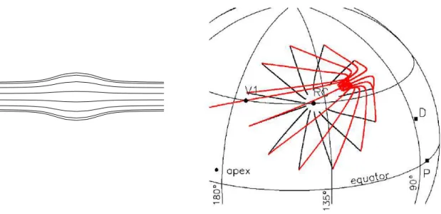
of the HP is called draping. A simple model of such draping may be developed by assuming that the HP is stationary and impenetrable both to the LISM and ISMF. Analytical solutions for such simple cases as a spherical or cylindrical obstacles were used to estimate the “draping factor,” i.e., the ratio of the maximum draped field strength to the strength of the unperturbed field (see [103]). One simplified solution to the SW–LISM interaction was proposed in [18] who considered the propagation of the spherically symmetric SW into a strongly magnetized, high plasmaβ

sur-rounding medium at rest. An astrosphere is formed in this case with the shape of the astropause determined by the equality of total pressures on its surface. The external magnetic field confines the

stellar wind creating a central cavity with two oppositely directed channels parallel and antiparallel to the magnetic field (see Fig. 10, left panel).

In [79], an analytical solution was proposed for a magnetic field frozen into the plasma flow, corresponding to another model of Parker: the incompressible axially-symmetric flow with the scalar velocity potential in the formΦ(r) = u0(z + q/r), where r and z are two cylindrical

coor-dinates, andu0 is constant and equal to the LISM velocity atr → ∞. To remain in the framework

of the analytical solution, the effect of the magnetic field on the plasma flow was neglected. For a slightly more general form of the flow potential [104], the solution for the magnetic field frozen into the flow was reduced to a single ordinary differential equation [105, 106]. However, these solutions are not fully consistent: at a distanced from the boundary of the model astrosphere the

field strength diverges as1/d1/2leading to infinite energy. This issue is caused by the presence of a stagnation point in the flow [107, 108].

Clearly, more realistic models for the description of the plasma flow and magnetic field in the vicinity of the heliospheric boundary are based on numerical solutions of MHD equations with proper source terms describing charge exchange between ions and neutral atoms. A number of references are given in this paper (see also [109] and references therein). It should be understood, however, that certain care is required to interpret numerical simulations of the magnetic field drap-ing if the HP is smeared by numerical viscosity and resistivity. This is especially true because of the necessity to correctly identify the neutral atom populations inside the HP structure. This is the case, of course, only for multi-fluid (non-kinetic) models that describe the neutral atom transport throughout the heliosphere (in [110], this is done by tracking the HP with a level-set method). The idea that the ISMF always becomes nearly equatorial at the heliopause in the V1 trajectory direction [111] is not supported by other numerical simulations [110, 112, 49]. From this view-point, exact solutions, however simplified, provide a useful supplement to numerical simulations. Parametric simulations are of importance to understand the evolution of numerical solutions. This approach was used recently in [100] to explain the puzzling observation of a very small change in the magnetic field elevation angle by V1 while crossing the heliospheric boundary [28]. The approach was chosen to track individual magnetic field lines and analyze them in projection on the celestial sphere. Consider a magnetic field line passing through a chosen point just outside the HP. As long as this line remains close to the HP it represents the draped magnetic field. Ultimately, the line departs from the vicinity of the heliopause and starts to approach the direction of the unper-turbed field. As a consequence, the projection of such line onto the celestial sphere approaches the points representing the inward and outward directions of the unperturbed field. For the strong-field Parker’s model of the astrosphere, the projections of magnetic field lines are great circles on the celestial sphere. If this model were applicable to the heliosphere, it would provide an immediate explanation to the small change in the magnetic field direction across the HP. As the V1 trajectory and the unperturbed magnetic field direction are very close in latitude and not widely separated in longitude, it is argued in [100] that the angle between the HMF and ISMF at the HP should be small.

The Sun is moving relative to the LISM. However, a hypothetical heliosphere obtained under the assumption of a very strong ISMF (20µG) will have draped magnetic field lines deviating only

slightly from great circles (see black lines in the right panel of Fig. 10. The angle between the projection of the draped field line and the heliographic parallel at V1 are still small. For an ISMF strength of 3–4µG, consistent with V1 observations, the draped magnetic field lines obtained from

Figure 10: Left panel) Magnetic field lines in the Parker model of the astrosphere confined by the magnetic field. When projected on the celestial sphere, the field lines become great circles connect-ing the unperturbed field and anti-field directions. (Right panel) Projections of the magnetic field lines in heliographic coordinates for two models of the heliosphere, corresponding to the ISMF strength of 20µG (thick black lines) and 4 µG (red lines) [100]. Also shown are the directions of

the V1 trajectory, the IBEX ribbon center (RC), the magnetic field measured by V1 before (P) and after (D) it crossed the heliopause, and the interstellar helium inflow (apex).

lines). However, this deviation remains small in the nose of the HP, as well as in the V1 trajectory

direction. The projection of the draped magnetic field line passing through V1 is at a small angle with respect to the heliographic parallel at this point, and this angle is close to the one observed by V1. It is argued in [100] that this is because the shape of the heliopause at its nose is roughly similar to a spherical shell resembling the stellar wind cavity in the Parker model. This is clearly not true in the heliotail.

Another region where the draped ISMF lines should be expected to have similar structure regardless of the ISMF magnitude, |B∞, is the vicinity of the so-called BV -plane [113, 114],

which is determined by the velocity and magnetic field vectors in the unperturbed LISM. The direction of V∞ is determined from the neutral He observations [115, 116, 98]. If B∞is directed

into the IBEX ribbon center (according to [99], the accuracy of this statement increases withB∞),

the BV -plane is approximately coincides with the interstellar hydrogen deflection plane (HDP,

see [117, 118]), which is formed by the H-atom flow directions in the unperturbed LISM and in the inner heliosphere. In the projection onto the celestial sphere, the BV -plane is a great circle

linking the unperturbed magnetic field and anti-field directions and passing through the helium inflow direction. If the ISMF-HMF coupling across the HP is ignored, the symmetry would require that magnetic field lines that start close to theBV -plane create a symmetric pattern only weakly

5.3

The possibility of a data-driven model of the outer heliosphere

The possibility of developing a data-driven model of the outer heliosphere was not even consid-ered 10–15 years ago. Now, because of the observations performed by the Voyagers, SOHO, and

IBEX, this has become a possible, albeit very challenging, task for theorists. Paper [99] is an

example of a systematic approach to fit multiple data sets. Earlier efforts have focused mostly on one or two challenging questions raised by observational data, e.g., negative radial velocity component at V1 in the inner heliosheath before the HP crossing [91, 87], fitting the IBEX ribbon [69, 26, 119, 120, 121], using the HDP to constrain the orientation of theBV -plane and the

distri-bution of radio emission sources observed by the plasma wave instrument (PLS) onboard Voyagers [122, 123, 124], using the ISMF draping results from V1 measurements to adjust the angle between

B_{∞ and V∞as well as|B∞| in simulations [125, 126, 113, 127, 128], or trying to adjust the SW}

and LISM properties in order to fit time-dependent observations along the spacecraft trajectories. In [99], the boundary conditions in the SW and LISM were chosen to (1) get the best fit to the IBEX ribbon; (2) reproduce the magnetic field angles observed by V1 in the HP draping region; (3) ob-tain the HP at the heliocentric distance consistent with V1 observations; (4) reproduce the density of the neutral hydrogen atoms at the heliospheric termination shock, which can be derived from

Ulysses observations of PUIs [129]; (5) ensure that theBV -plane is in agreement with SOHO

ob-servations (uncertainties in the HDP determination are discussed in [27]). The model used in [99] is based on the kinetic treatment of hydrogen atom transport throughout the heliosphere, which is very important to have a more realistic filtration ratio of the LISM hydrogen atoms near the HP. In [130], a detailed comparison of the 5-fluid and kinetic models of the SW–LISM interaction was made. It showed that the results are qualitatively agreeable, with only a slight shift in the quantity distributions along different lines of sight. On the other hand, kinetic modeling of a realistic solar cycle is more time-consuming. To improve statistics and reduce numerical noise typical of the Monte Carlo simulations, one needs either assume the presence of a longer cycle (in multiples of the usual solar cycle) and perform averaging based on the repeated simulation of such cycle [131] or perform averaging over multiple implementation of the same period inside the solar cycle period [120]. We note in this connection that a solar cycle model [85] based on Ulysses observations was successful in reproducing both the heliocentric distance and the time at which V1 and V2 crossed the TS. This means that taking into account solar cycle effects is of major importance. Addition-ally, the model of [99] used the solution of the SW–LISM interaction problem based on a single plasma fluid model where PUIs born in the process of charge exchange with neutral atoms were added to the mixture of ions preserving the conservation of mass, momentum, and energy. The separation of PUIs and thermal SW ions was made at a post-processing stage which involved a sophisticated procedure to fit IBEX observations in different energy bands covered by the space-craft. This procedure is very important for understanding the energy separation between ions (see, e.g., [35, 132, 133]), but ignores the dynamical effect of PUIs on the heliospheric interface. While the necessary improvements to the fitting procedure are well understood, their implementation will be rather laborious. It is known that treating PUIs as a separate ion population results in a nar-row heliosheath: the TS heliocentric distance increases, while the HP moves closer to the Sum [36, 37]. In [99], the HP stand-off distance in the V1 trajectory direction was adjusted by choosing the SW/LISM stagnation pressure ratio and the HMF and ISMF strengths and direction. In the future, V1 and V2 measurements should be used to improve the quality of the MHD-kinetic fitting of data from multiple sources.

5.4

The heliotail

An additional constraint on the LISM properties is provided by multiple air shower observations of the 1–30 TeV GCR anisotropy [134, 135, 136, 137, 138]. According to [9, 139], this anisotropy is affected by the presence of the heliosphere, especially due to the ISMF modifications in the heliotail and bow-wave regions. It is clear that the heliotail should be very long to produce an observable anisotropy of 10 TeV cosmic rays whose gyro radii, assuming protons, may be as large as 500 AU.

Paper [7] considered the flow in the heliotail and compared simulation results with theoretical predictions [5, 140] and numerical modeling [6, 141]. The main conclusion is that the heliotail is very long, likely about2 × 104

AU. If the LISM is superfast magnetosonic (the flow velocity is greater than tghe fast magnetosonic speed), which happens if B∞ is not too strong (less that

∼ 3 µG), the SW flow becomes superfast at distances of about 4 × 103 _{AU along the tail. It was}

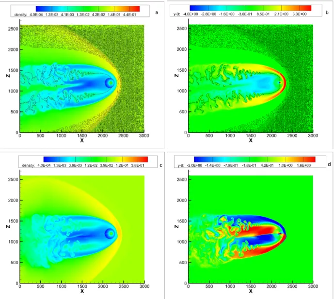
found that a kinetic treatment on neutral hydrogen atoms becomes critical. This is not surprising since multi-fluid approaches (see, e.g., [40, 142, 130]) are more likely to produce artifacts at larger distances. In multi-fluid models, the flow of neutral hydrogen atoms is described by multiple sets of the Euler gas dynamics equations, each for every population of neutrals born in thermodynamically different regions. In particular, it was found in [7] that there is a region in the heliotail where the SW flow remains subfast magnetosonic in contrast to the kinetic-neutrals solution. The reason can be understood if we look at the distribution of plasma number density in multi-fluid simulations from [7] shown in Figs. 11a,b. These figures show the density and the out-of-plane component,

By, of the magnetic field vector. In both panels, there appear to exist two lobes of enhanced SW

plasma number density, which are separated at x ≈ 1, 500 AU by a region with substantially

different parameters attributed to the LISM in [6]. It was shown long ago in [5] that these lobes are due to the concentration of the SW plasma inside the Parker spiral field line diverted to the tail when the SW interacts with the HP. The central spiral originates where thez-axis crosses the

inner boundary. Both Bx and By are zero along this line, shown in Figs. 11a,b, until it exits the

supersonic SW outside the TS. This critical magnetic field line deflects tailward with other spiral field lines. According to [143, 5], the plasma inside the spiral field is subject to a kink instability. As a result, the lineBy = 0 exhibits rather chaotic behavior. As shown in [7], the above line carries

an electric current, which increases considerably when the plasma distribution becomes unstable. Once the Parker field is destroyed by the kink instability, the necessity of plasma concentration inside the lobes disappears. However, as seen in Figs. 11a,b, they still exist at x = 0, although

their width increases. This behavior is in a drastic contrast with the solution where the transport of neutral hydrogen is treated kinetically, by solving the kinetic Boltzmann equation with a Monte Carlo method [7, 141] (see Fig.12). When neutral atoms are treated using a multi-fluid approach, there is little charge exchange in the region separating the lobes. This is because the LISM neutral atoms, whose flow is governed by the pressure gradient, do not cross this region. On the other hand, kinetic neutrals always cross the separation region because of their thermal velocity. Notice that although the simulations in [7] demonstrate some separation between the lobes, it is much smaller than in [6], and the heliotail is considerably longer.

It is interesting to notice in this connection that short heliotails, such as observed in solutions [6], are not favorable for creating flux anisotropies in 1, and especially 10, TeV GCRs. A heliotail of less than 1,000 AU long would have little effect on those GCRs because of their large gyroradius. The assumption of the unipolar heliospheric magnetic field made in [6] requires special discussion.

Figure 11: (Top row.) The distributions of the (a) plasma number density and (b) out-of-plane component,By, of the magnetic field vector in the meridional plane in the multi-fluid simulations

without interstellar magnetic field, unipolar heliospheric magnetic field, and all other parameters from [6]. (Bottom row.) The same as in the top row, but assuming the helisphereic current sheet is flat, i.e., there is no angle between the Sun’s rotation and magnetic axes. Densities are in particles per cm3

Figure 12: MHD-plasma/kinetic-neutrals simulation of the SW–LISM interaction from [7]. (Top panel) The shape of the heliopause for two different ISMF strengths is shown (yellow and blue forB∞= 3µG and 4 µG, respectively). (Bottom panel) HMF line behavior initially exhibits

a Parker spiral, but further tailward becomes unstable. Also shown are ISMF lines draping around the heliopause. The distribution of the plasma density is shown in the semi-transparent equatorial plane. [From [7] with permission of AAS].

While it is clear that the region of the SW swept by the HCS is impossible to resolve when the sector width becomes small, which is inevitable when the SW is decelerated by the HP to very small velocities, it is not quite clear why the solution with the removed HCS is better. In Ulysses-based, time-dependent simulations of [7], the HMF along the Voyager trajectories is reproduced on the average, even though the HCS dissipates, which would not be possible if the magnetic field was assumed unipolar. It is worth noticing that V1 was in a region of very small, even sunward, radial velocity component for two years before it crossed the HP. As previously mentioned, when the numerical resolution is sufficiently high, the HCS does not simply dissipate due to numerical effects. The plasma and magnetic field behavior in the region swept by the HCS becomes chaotic likely due to the tearing mode instability, which is inevitably numerical in MHD simulations. As a consequence, the magnetic field strength becomes rather weak and the sector structure disappear. This is in agreement with V1 observations which otherwise would show sector crossings much more frequently. In our opinion, it is possible that the sectors observed by V1 are more likely due to stream interaction and solar cycle effects. Such sectors are much less frequent than those related to the Sun’s rotation. It is possible that the spacecraft are crossing such sectors even in regions where the classical HCS does not exist. When the heliospheric field is assumed to be unipolar, its strength may be greater than in V1 observations. Further, assuming a unipolar field necessarily assigns an incorrect sign to the HMF below or above the magnetic equator. Additionally, solar cycle effects disappear, despite being an important ingredient of the SW flow.

The HCS is nearly flat close to solar minima. As seen from [144], it bends into one of the hemispheres depending of the direction and strength of the ISMF. The flat-HCS case easily can be treated numerically and is therefore a good test for unipolar simulations. Figures 11c,d show the solution similar to that shown in the top row of this figure, except that the HCS is flat in the supersonic SW. It is seen that although the lobes do reveal themselves at small distances from the Sun, there is no separation between them farther along the tail. This happens because the HCS in the tail is affected by the unstable SW flow.

Another test for the unipolar HMF assumption would be to allow the SW variations related to the solar cycle. The solution obtained under these assumptions is shown in Fig. 13. We see here a drastic change in the entire structure of the heliotail flow. The lobes disappear completely. On the contrary, the SW plasma is more dense near the equatorial plane. This is not surprising because

Figure 13: Clockwise, the distributions of plasma number density (in cm−3) and temperature (in K), they-component of the magnetic field and its magnitude in the SW–LISM simulation in our

solar-cycle simulation assuming unipolar heliospheric magnetic field. The top left panel also out-lines the HP.

Figure 14: The heliotail in the multi-fluid simulation which takes into account solar cycle effects. The distributions ofBy are shown in the meridional (left panel) and ecliptic (right panel) planes.

The HP looks rather thin beyond 2,000 AU. In reality it is rather wide latitudinally in the BV

-plane, but very thin in the direction perpendicular to that plane. The LISM boundary conditions for this problem are taken from [99].

the slow SW is denser than the fast wind near the poles. This solution makes questionable the idea of a short, “croissant”-like heliotail shown in [6]. In other words, the heliotail structure becomes completely different from that described in the analytical studies of [5, 145]. The latter also did not take into account charge exchange, while it is known that even the original Parker solution [18], which described the SW propagation into the magnetized vacuum, is only partially valid in the presence of interstellar neutrals (see [109]). This is because charge exchange does not allow the SW to propagate upstream indefinitely. One can see from Fig. 13 that the solar cycle smears out more subtle effects related to the SW plasma collimation within the Parker magnetic field swept by the flow into the tail. As shown in [144, 7], the HP usually rotates to become nearly aligned with theBV -plane. Black lines in the tail show that the instability of the HP flanks may produce local

protrusion that cross the meridional plane.

As shown in [7], the effects of the solar cycle are not only due to the changes in the latitudinal extent of the slow wind. Of importance are also changes in the angle between the Sun’s rotation and magnetic axes, as well as the change of the magnetic polarity of the Sun every solar cycle at maxima. In Figure 14, we show the distribution of the y-component of the magnetic field vector

in the meridional and ecliptic planes for a simulation using parameters from [99] forB∞ = 3 µG.

Note the similarity of the shape of the heliotail to that estimated earlier by [140].

Solar cycle simulations of the heliotail presented in Figs. 11 and 13–14 are obtained with a multi-fluid model. No characteristic wave reflections have been observed from the exit boundary. Time-dependence creates conditions where no fluid dynamics artifacts in the neutral H flow are observed.

The numerical analysis of [146] demonstrates that solar cycle effects, especially the presence of slow and fast wind regions, are seen in the ENA fluxes observed by IBEX from the tail direction.

This requires no collimation of the SW plasma that is observed in simplified models of the helio-sphere. Additionally, as mentioned above, the short heliotail obtained in numerical simulations [6] is incompatible with the idea that the multi-TeV cosmic ray anisotropy is affected by a large perturbation of the ISMF due to the presence of the heliotail.

By fitting the anisotropy of multi-TeV cosmic rays observed in air shower observations by the Tibet, Milagro, Super-Kamiokande, IceCube/EAS-Top, and ARGO-YGB teams (see references in [9]), we can derive restrictions on the LISM properties as found in [147, 139, 9]. Additionally, it is suggested in [148] that ion acceleration due to reconnection in the heliotail may affect observed anisotropies.

The main result of our heliotail study is three-fold:

• Even our multi-fluid model, when run with the unipolar heliospheric magnetic filed

assump-tion, shows results different from [6]. This is shown in Figure 10. One can only guess about the reasons for that. A possibility is the implementation of the subsonic exit boundary conditions.

• In [7], we have found that in agreement with [149] and [141], the SW flow becomes superfast

magnetosonic again at distances of about 4,000 AU. In such cases, no boundary conditions are necessary at the exit boundary. In the absence of solar cycle effect, this happens only if neutral atoms are treated kinetically, but never if they are treated with a multi-fluid approach. This is our explanation of the qualitative difference between MHD-kinetic and multi-fluid results.

• All of the above conclusions become irrelevant when solar cycle effects are taken into

ac-count. As shown in Fig. 13, the collimation of the SW within two polar lobes disappears even if the heliospheric magnetic field is assumed unipolar, which is the necessary condition for obtaining a “croissant”-shaped heliosphere with the LISM between the lobes. We obtain one single heliosphere. Instead of concentrating inside the lobes, the SW has higher density near the equatorial plane, where the slow SW is. From this standpoint, the above two con-clusions have only theoretical importance because they do not take into account one of the basic features of the SW flow: the solar cycle.

• As the SW propagates tailward, both thermal and nonthermal ions continue to experience

charge exchange which substitutes them with the cool LISM ions until the plasma temper-ature in the tail becomes uniform and the heliopause disappears. As seen from [7], the he-liopause should become very narrow, while being aligned with theBV -plane. Newly created

neutral atoms, because of their large mean free path will be leaking through the HP surface into the LISM and ultimately reach thermodynamic equilibrium with the pristine LISM. The assumption of a unipolar field in the tail is damaging for determination of GCR fluxes coming from the heliotail. There is no imperative to running the code with the variable tilt between the Sun’s magnetic and rotation axis. This inevitably results in the HMF dissipation in initially sectored regions of the SW. Clearly, only models that involve SW turbulence can correctly address this issue. Local kinetic simulations may be useful to establish the dissipation rate and in this way supplement global models. On the other hand, as shown in [85], the HMF at Voyagers can be reproduced on the average even if some sector structure is lost.