Designing molecules possessing desired physical property values

(1)

Designing IVlolecules Possessing Desired Physical

Property Values Volume 1

by

Kevin

G.

Joback

B.E. Stevens Institute of Technology 1982 S.NI. Ivlassachusetts Institute of Technology 1984

Submitted to the Department of Chemical Engineering in Partial Fulfillment of the

Reqtlirements of

Doctor of Philosophy at tIle ~lassachusettsInstitute of Technology

©

rvIassachusetts Institute of Technology 1989

©

I{e\·in G. Joback 1989

~jgnatttre of Author---7,....<..,..7€:...~W_:,,::·...."""""'-/---.<Z...1~~._~:>,..?"'""""---.>oIIIIjoI~~e-t....< ...'.,.;;",<..."'<'"-,--_ _

Department of Chemica! Engineering June 27, 1989 Ccrtifir3 by ,~,.<o-..·-,,--~~V-_+,I->+.~.If--·-~--v--+rrl---_ _~

Professor Geort~eStephanopoulos Thesis Supervisor :\ccept.ed

by

_

VnL.!-1\1ASSACHUSmsIr~Sl1tUT.E OF1ECHNOtiJGY

OCT 3

1989

~

\Villianl

wI. Deen

Cllairperson, Departm(~ntalGradtlate Committee

(2)

Abstract

TIle search for new compounds possessing unique and improved properties is an im-portallt aspect of chemical engineering. Much of this search is COllducted at the exper-imental level. Chemists synthesize and test thousands of compounds searching for a ne,v pllarmaceutical and tens of thousands searching for a new insecticide. Computer imI)}ement.ation of techniques which determine physical and chemical properties now a.llo\v much of this search to be performed at a computational rather than experimental le\·cl.

Numerous techniques exist for estimating a compound's physical property values given its molecular structure. !vIy thesis research has focused on using these estimation tech-niques in the inverse manner: specifying desired physical property values and designing the molecular structure of compounds which possess these values. I present a method-ology which performs such a moleclliar design.

TIle methodology consists of six steps:

1.

Problem Formulation:

problem formulation involves deterlnining constraints on important physical properties.

2. Target Transformation:

equation oriented physical propertyestimation tech-niques are used to propagate these constraints to constraints on properties esti-mated by group contribution techniques.

3. Group Selection:

the heart of the methodology consists of two procedures: one interactive and one al1tomatic. Both are based upon group contribution estimation techniqlles. The interactive procedure uses interactive graphics.

Vi-sually representing the problem allows a moleclliar designer to use his or her own knowledge to guide thesearcll. The automatic procedure uses a hierarchical gen-erate alld test paradigm to exhaustively and efficiently search a large number of molecules.

4. Molecule Enumeration:

the design procedures produce collections

of

groups. These groups can be connected in several ways to produce complete molecules. All possible \vays of connecting these groups are enumerated giving all possible molecular structures.

5. Molecule Screening:

the design procedures utilize knowledge at the group level of detail. After enumeration we have complete molecules and thus can use m.olecule level knowledge. This knowledge is in the form of rules specifying molecular substructures which are not allo\ved in the designed molecules.

(3)

6. Final

Evalu~tion: it is sometimes necessary to use simplified physical property estinlation models to design molecules. The final step of the metllodology is to further prune the designed molecules using very accurate estimation tecllniques.

~Jy' tllesis presents these six methodological steps. Case studies in refrigerant design, polj·mer design, sol~'entdesign, and drug design demonstrate the methodology.

(4)

...

3

1.2

Incentive . . 3 1.3 Overview . . . 4 1.4 Scope

...

6

2 Previous Work 8

2.1 Estimating Physical Properties 8

2.1.1

Pattern Recognition

..

9

2.1.2 Topological Techniques . 15

2.1.3 Group Contribution Techniques

16

2.1.4 Eql1ation Oriented Techniques . 19

2.1.5

Moleclliar Modeling Techniques 20

2.2

Selecting Chemical Products . 23

2.2.1

Godfrey

24

2.2.2

Francis.

25

2.2.3

Berg

..

25

2.3

Designing Chemical Products

....

27

2.3.1 Solvent Design

28

2.3.2

Polymer Design 30

2.3.3

Polymer Coatings Design. . . 33

2.3.4

Drug Design . . 36

(5)

2.5 DENDRAL

. .

.

· ....

43

2.6

Illterval Arithmetic

49

3 fvlodeling Molecular Design 51

3.1 Constraint Elucidation 51

3.2

Property Estimation

52

3.3

Molecule Gerleration

52

...

71

4.4.3

Physical Property Constraints . 72

4.4.4 State . .

72

4.5

Summary

...

72 5

Target Transformation

73 5.1 Estimation Procedures 73

5.2

Selection Criteria

75

5.3

Restriction . 0 • • •

75 .5.4

Group Consistency

. . . . .

76 6 Automatic Design

79

6.1 Generate and Test

80

(6)

6.2.1 ~lo1ecules

82

6.3

The Tester . . c • • 83 6.3.1 Property Constraints 83

6.3.2

Structural Constraints

84

6.3.3 Chemical Constraints . . 91

6.4

Algorithm . . .

· ...

92

6.5

A Combinatorial Explosion.

94

6.6

i\fcta-G roups 95 6.7 ~/leta-Ivlolecules

95

6.8

Meta- Contributions 97 6.8.1 Intervals . . 97

6.9

~1eta-Properties . .

98

6.9.1 Excess Width

....

100

6.9.2

Causes of Excess Width

101

6.10 Metal-Algorithm . . . 103 6.10.1 Division Strategies 108

6.11

Algorithm Evaluation .

· ...

113

7 Interactive

Design

130 7.1 Procedure Basis • • • • • e 131 7.2 Const.raint Visualization 145

7.3

Interactive Pruning . . . .

...

148

7.4

Cognitive Model of Interactive Design. 151

7.4.1 Representation

..

151

7.4.2

Focus of Attention

· ...

154

7.4.3

Pattern Recognition 154

7.4.4

Zooming . . . 155

7.4.5

Design Facilities . . 155

7.4.6

Cognitive Sample .

....

156

(7)

10 Molecule Evaluation 8.4 Implementation Difficulties. 8

Enumeration

8.1 The Problem 9 Molecule Screening 9.1 The Problem . .

166 ...

167 168 170 176

178

179

180 183

....

184

185

186 189 190 192 192 194 195 198 198 198

200

201

203

203 205 Combinatorics . Enumeration Procedure Group Formation . 9.2 Disallowed Stlbstructures . 9.3 Substructtlre Representation

9.4 Substructure Identification Procedure .

9.4.1 Stage 1: Matching Atom and Bond Types 9.4.2 Stage 2: Matching Atoms and Bonds . . . . 9.4.3 Stage 3: Match Indiviual Atom-Bond Connections 9.4.4 Stage 4: Match

All

Atom-Bond Connections . . 9.5

11.5 Freon 12 .

11.6 Problem Formulation 11.7 Target Transformation

11.7.1 Tra.nsformation for Interactive Design.

11.7.2 Resulting

Properties

and

Groups . . . 11.7.3 Transforma,tion for Automatic Design. 11.7.4 Resulting Properties and Groups . . .

8.2

8.3

11 Refrigerant Design 11.1 Refrigeration . . 11.2 Current R.efrigerants

11.3 Problems with Chlorofluorocarbons

(8)

11.8 Interactive Design . . . . . 11.8.1 Interactive Results 11.8.2 Replacing Chlorine 11.9 Automatic Design . . . . . 11.9.1 Automatic Results 12 Polymer Design 12.1 Ie Packaging . . . . . 12.2 Current Encapstllants . 12.3 Problem Formulation . 12.4 Target Transformation

12.4.1 Transformation for Automatic Design. 12.4.2 Consistent Groups 12.5 Automatic Results 13 Solvent Design 13.1 The Problem 13.2 Current Solvents 13.3 Problem Formulation . 13.4 Target Transformation 13.4.1 Group Contributions 13.5 Interactive Design . . . . . 13.5.1 Homologous Series

13.5.2

Solvent 1fixtures .

13.6 Automatic Design using UNIFAC 14 Drug Design

14.1 Steps in Drug Design . 14.1.1 Target Biological Properties

14.1.2 Identification of "Lead" COlnpounds . . . . 14.1.3 Analog Synthesis and ~lodel Development

206 207 ~13

213

216

221

222

223

224

225

227 229

235

237

239

240

246

247 250 250 254 256

257

257 258 258

(9)

14.1.4 Optimization of Drug Potency. 14.2 The Problem . . . . . 14.3 Problem Formulation . 14.4 Target Transformation 14.5 Interactive Design . 15 Conclusions 16 Recommendations 16.1 Structural Constraints 16.2 Meta-Group Strategies

16.3 Design Methodology Cooperation 16.4 Specific Estimation Techniques 16.5 ~1olecular Display . . . . A Estimation Techniques

A.l Normal Boiling Point .

A.I.I Group Contribution Technique A.l.2 Equation Oriented Technique

A.2

Reduced Boiling Point .

A.2.1 Group Contribution T~chnique

A.3 Critical Temperature .

A.3.1 Equation Oriented Technique

A.4

Critical Pressure .

A.4.1 Group Contribution Technique A.4.2 Equation Oriented Technique

A.,)

Vapnr Pressure .

A.6

Acentric Factor .

A.6.1 Equation Oriented Technique A.7 Enthalpy of Vaporization at

Tb. . . . .

261 262 263 266 267 270 272 273 273

273

274

289 289 291 291 293 294 294 296

296

297 297 299

300

301 301 302

(10)

A.7.1 Gl'onp Contribution Technique A.7.2 Equation Oriented Technique A.8 Enthalpy of Vaporization . . . .

A.S.I Equation Oriented Technique

A.9 Factors .

A.9.l

F

1 Group Contribution Technique.

A.9.2

F2

Group Contribution Technique . .

A.9.3

F

2 ASSllmption .

A.9.4 F3 Group Contribution Technique.

A.IO Ideal Gas Heat Capacity . ..~.lO.l Group Contribution Technique A.I0.2 Equation Oriented Technique A.l1 Liquid Heat Capacity. . .

A.11.1 Equation Oriented Technique A.12 Glass Transition Temperature . . . . .

A.12.1 Group Contribtltion Tecllnique

A.13

Gas

Permeability .

A.13.1 Group Contribution Technique

A.14 Volume Resistivity .

A.I5 ~101ar Polarization .

A.15.1 Group Contriblltion Technique

A.16 Molar Volume .

A.16.1 Group Contribution Technique A.17 Molecular Weight .. A.IS Polymer Thermal Conductivity

A.IS.! Equatioll Oriented Technique A.19 Solid Molar Heat Capacity .

A.19.1 Group Contribtltion Technique

A..20

Rao

Function .

302 305 305 305

306

308

310 310 312

312

313 315

316

316 317

321

321 324

325

326

329

335

338 339

340

343

(11)

A.20.1 Group Contribution Technique A.21 Solubility Parameters .

A.21.1 bp Group Contriblltion Technique

A.21.2

6h

Group Contriblltion Technique . A.~;2 Drug Design . .

A.22.1 O'At

A.22.2 1r • •

B Estimation Procedures

B.I Pvp Estimation Procedures

B.1.1 Interactive Estimation Procedure B.l.2 Automatic Estimation Procedure B~2 Hv Estimation Procedures . . . .

B,.2.1 Interactive Estimation Procedure B.2.2 Automatic Estimation Procedure B.3

C

_PL Estimation Procedures .

B.3.1 Interactive Design Procedure . . B.3.2 Automatic Design Procedure . . . .

C Physic~p.l Property Ranges

e.1

Critical Temperature

C.2

Critical Pressure

...

C.3 Reduced Boiling Point

C.4

Normal Boiling Point . D

Mono"tonicity Identification

D.I Acentric Factor D.2 Vapor Pr:~ssure D.2.1 PtJp Monotonicity D.2.2 h ~1onotonicity D.2.3

G

~fonotonicity .

343

346 347 348

350

352 352

355

35.5 . . . . .

356

....

359

....

359 359

. . . .

361 361 363 367 367 369 369 369 373

...

374

377 378 380 380

(12)

D.2.4

k

~Ionotonicity E

Factor

Analysis

E.l Principal Component Analysis . E.2 Factor Analysis

· ...

E.3 Factor Analytic Studies. . E.3.l Cramer

_·

_.

E.3.2

Klinewicz

E.3.3 Joback .

_{· .}

E.4 Dinlensional Reduction E..S Group Contributions

381 382 383

384

384 385 387 389 391 392

(13)

List of Figures

2.1 General Structure of 9-Anilinoacridine . 2.2 Critical Solution Temperatures of Three Liquid ~[ixtures 2.3 Solubility Parameter Scale used in Coatings Design 2.4 Initial Penicillin for rvlodification by Drug Design 2.5 Irlput Data for Hel1ristic DENDRAL .

2.6 General Design ofHeuristic DENDRAL's Five Nfajor Sections 4.1 Selectivity ofS for the Separation of B from A.

4.2 Basic Refrigeration System . . . . . 4.3 Hypotlletical Refrigeration Cycle

6.1 Molecules DemOIlstrating Structural Constraint 3 6.2 Example Chemical Constraint . . . . .

6.3 Automatic Design Algorithm Structure 6.4 Automatic Design ~1eta-Algorithm ..

12 26 35 39

44

45 59 63

64

87 91 93 109 7.1 Graphical Representation of Constraints in a Physical Property Space. 135 7.2 Graphical Representation ofTb and Tm Contributions . 136

7.3 An Interactively Designed ~Iolecule: Chloropropane . 137 7.4 Simultaneous Design in Multiple Physical Property Spaces 140

7.5 Pc-T*

_b: Design Space for Acentric Factor Constraint 143

i.6 Two Dimensional Space Showing Four Constraints. 147 7.7 Effect of ~.fodifying6.Hv Constraint on the Feasbile Region. . 149

·1.8

Expanded Feasible Region Formed by Relaxing Constraints by 20% 150

(14)

7.9 Interactive Design Implementation Display 158

7.10 Temporary Group Vector . . . . 159

7.11 Restriction of Displa)red Groups 160

7.12 Choosing the 1\lethyl Group Vector 162

7.13 Angle Restriction on Group Vectors . . 163

7.l~t Choosing a Second lerminator . 164

11.1 Basic Refrigeration System . . . . 193

11.2 Hypothetical Refrigeration Cycle 194

11.3 Refrigerallt Design: Interactive Design Space .

....

208

11.4 Refrigerant Design: Freon 12 . . . 209

11) Refrigerant Design: Example rvlolecule 210

11.6 Chlorine Group Vector

...

214

11.7 Candidate Groups for Chlorine Replacement 215

13.1 Schematic of Solvent Extraction . . . .

240

13.2 Example fJp Vs. OR Parameter Space . .

...

244

13.3 Example Dp vs. 6H Parameter Space. .

245

13.4 fJp vs.

6

11 Design Space . . .

246

13.5 Solubility Parameter Design Space

....

248

13.6 Example Solvent 249

13.7 Solvent ~Iixtures 251

13.8 Interactive Design of Solvent rvlixtures

...

253

14.1 Existing Antiallergic Sodium Cllrornoglycate . 262

14.2 "Lead" Compound for Drug Design

263

14.3 (fAt

'-5.

1r Drug Design Space . . . . 268

14.4 Two High Activity l\feta-Substituents .

269

(15)

List of Tables

1.. 1 Pllysical Property Dependence of Chemical Products 2.1 Some Estimatable Physical Properties ...

2.2

Specific Substructure Descriptors . . ..

2 ..3 18 Descriptors for Antitumor Activity Classification ...

2.4

X

and

Tb

Data for Alkanes

2..5 Alkane Grollp Occurrpl1cer

2.6 ~Gf,'298 Group Contribution

Estimation

Errors.

2.7 T

c Equation Orient~dEstimation Technique Errors 2..8 Properties Available from the Potential Energy Function

2.9

God.frey's Standard Solvents arld

rAiscibility

Number ..

2.10

Ordering of DeviatioIls from R.aoult's

Law

..

2.11 Groups Used in Solvent Design

2.12

Groups used in PGJymer Design

2.13 Group COiltributions used in Polymer Design. 2.14 12 Satisfa~tory Candidate Polymers .. 2.15

r.,filitary

Specificationd for Air Craft Coatings 2.16 Erosive Aircraft FJuid's

Solubility

Parameters 2.17 Input Data for QSAR A.nalysis . 2.18 QSAR Relationships R.egressed from Input Data . . 2.19 Estimated

Activity

for

QSAR Analysis ..

2.20 Heuristic DENDRAL's Identification Rules 4.1 Important Physical Properties in Solvent Design

2 10 13 14

17

18 19 21

23

24

28

29

30 31 32 34

35

39

40

41

47

58

(16)

.5.1 An Example Estimation Procedure 5.2 Group Sets for GCT-l and GCT-2 6.1 Initial Set of Groups . 6.2 Example Candidate !vlolecules 6.3 Combinatorics of Group Selection 6.4 Example Meta-GrOtlpS .

6.5

Tb

Group Contributions for ~Ieta-Group 2

6.6 Meta-Contributions ..

6.7 T

bValues for Four Meta-~101ecules

6.8 Tb Values

for

13 ~feta-Molecules

..

6.9 Hypothetical ~1eta-Groupsfrom Partitioning 4 Groups into 2 Clusters . 6.10 Partitioning 19 Groups into N Clusters

6.11 Maximum Number of rvleta-rvlolecules . 6.12 i\1aximum Number of Meta-fvlolecules .

6.13 Meta-Molecules Formed from 3 Meta-Groups . .

6.14 Maximum Number of Meta-Molecules Needing Testing 6.15 ~laximumNumber of Meta-Molecules Needing Testing 6.16 Pruning R.eslllts for k=44, n=3 Automatic Design . . . . . 6.17 Pruning Results for k=44, n=5 Automatic Design .

6.18 Example Pruning Percentage: 3 Occurrence 6.19 Example Pruning Percentage: 5 Occurrence

6.20 Average Number of Children Meta-Molecules Needing Testing 6.21 Automatic Design with 10% Average Pruning

6.22 Automatic Design with 10% Average Pruning 6.23 Advantage of Abstraction: MG2 Contains 1 GrOtlp

7.1 Example of Linear Group Contribution Estimation Techniqlles

7.2 L\Hvb Group Contribution Estimation Technique · · 7.3 Equations Relating Physical Properties to Factors . 8.1 Four Enumerated Molecules .

77

81 83 94

96

97

99

105

107

110 111 115 116 116 118 119

121

122

123 124 125 126 127 129

131

138 145 167

(17)

9.5 Atom and Bon.d Counts

8.2 Combinatorics of Bond Association

11.8 Refrigerant Design - Automatic Results

11.7 Literature Values for some Designed Refrigerants

169 176 179 182 182 183 185 196 199

203

206

211

Design -

Automatic Results . . . 11.1 Current Refrigerants . .

11.2 Physical Properties of Freon-12

11.3 COIlsistent Groups for Refrigerant Design .

11.4 Consistent Groups for Automatic Refrigerant Design

8.3

13.1 Acetic Acid Distribution Coefficients in Various Solvents 13.2 ](D fOf Several Homologous Series . . . .

13.3 Acetic Acid and Water Solubility Parameters . . 13.4 Liquid-Liqtlid Extraction Solvents .

13.5 Solvent Mixtures 13.6 UNIFAC Groups

13.7

Some

UNIFAC

Interaction Parameters

14.1 Dat~. for Initial 19 Analogs .

14.2 Comparison of Experimental and Model Activities.

238 239 250

251

252

254

....

254

264

265

(18)

14.3 Consistent Grollps for Drug Design

A.I

Estimated Physical Properties A.2 Tb Group Contributions

J\.3 Tbr Group Contributions

....

A.4 Pc

Group Contributions

A.5 ~Hvb Group Contributions .

A.6

F1 Group Contributions

....

A.7 F

2 Group Contributions A.8 F3 Group Contriblltions

A.9 C;v

Group Contributions. A.IO }~ Group Contriblltions .

A.II A and S Parameters for Pcrmachor Estimation

A.121r Group Contributions . . . A.13 Gas Permeability Estimates A.14

P

LL Group Contributions . .

A.15 ~Iolar Volume Group Contributions . .

A.16 Molar Volumes of Rubbery Amorphous Pol)'mers at 25°C. A.17 Molar Volumes of Glassy Amorphous Polymers at 25°C A.IS Molar Volume Group Contributions

A.19 AIw

Group Contributions . . . . _

A.20 Thermal Conductivities

of

Amorphous Polymers . . A.21 Cps Group Contributions .

A.22

U

Group Contributions . ~

A.236p Group Contributions . . A.24 Example 6p Estimation Errors

A.25 6h Group Contributions. . . . .

A.26 Example

6

h Estimation Errors .

A.270'AI

Group Contributions

A.281r Group Contributions . .

267 290 292 295 298 303

307

309 311 314 319 322

323

324 327 330 332 332 334 337 339 341 344 348 349

350

351 353 354

(19)

0.1 Pvp Estirnation Procedllre Errors - Interactive 357

B.2 Pvp

Estimation Procedllre Errors - Automatic 358

B.3 Hv

Estimation Procedure Errors - Interactive

....

360

B.-1 Hv Estimation Procedure Errors - Automatic 362

B.,5

C

_PL Estimation Procedure Errors - Interactive . 364

B.6 C

_PL Estimation Procedure Errors - Automatic .

366 C.l

Tc High and Low Sa~mple Values . . 368

C.2 Pc

High and Low

Sample Values . . 370

C~3 T_br High and Low Sample Values

....

371

C.4 Tb

High and Low Sample Values . . 372

D.l Acent.ric Factor . 375

E.l Pllysical Properties as Functions of BC(DEF) Factors . . . 386

E.2

Statistics for

BC(DEF)

Factors - Physical Property Relationships

388

E.3 Physical Properties in I{Iincewicz's Factor Analytic Study

E.4 Percentage Variance Explained by Klincewicz's Factors

E.5

Klincewicz's Factor Analysis

Data

Summary Statistics E.6 Loadings

for

I{ljncewicz's Three Factor Model .

E.1

Physical Properties in Joback's

Factor

Analytic Study.

E.8 Total

Variance Explained

in

Joback's Factor Models . .

E.g

Physical Property - Factor Relationships . . .

E.I0 Percentage Variance Expla.ined by 2 Factors

388

389

390

391

391 392 393

(20)

Notation

Physical Properties

C;,a , C;,b'

C;,c,

C;,d· · · ..

Coefficients of a cubic fit of ideal gas heat capacity.

C

_PL ••••••••• • •••••••••••••••••• Liquid Heat Capacity.

c; ...

Solid heat capacity.

c;v

Ideal Gas Heat Capacity at 298K.

CR(k,

n)

a • • • • • • • • • • • • • • • • • • • • • • the number ofways

n

objects can be chosen from aset of

k

objects ignoring the order of choice and allowing repetitions.

F

1 • • • • • • . • • • • • . . • • . • . • . . . • . . • •• Factor 1.

F

3 • • • • • • • • • • • • • • • • • • • • • • • • • • • •• Factor 3.

~G/t298

· · · •· · · ..

Standard Gibbs Energy of Formation at 298K.

~Hf,298

..•...•....

Standard Enthalpy of Formation at 298K.

6.H,n . . . ..

Enthalpy of Fusion.

~lIv. ...•... Enthalpy ofVaporization.

6.1I

vb •••••••••••••••••••••••••• Enthalpy of Vaporization at the normal boiling point.

[(D. · · · .. · .. · · · · . · · .. Equilibrium distribution coefficient.

!vI . . . ..

~101ecularweight.

mB •.•••.•••.•.•.•..•...•.. Distribution coefficient of solute B.

Al R . . . ..

Molar Refractiort.

(21)

Pc

Critical Pressure.

plso log ofthe concentration producing a 50% inhibition.

PLL · · · .. ~lolar polarizability.

P(02) . . . .. . . .. .. Permeability ofoxygen through polymer.

Pup · .. · · · · .. Vapor Pressure.

R ~ _.. Volume resistivity.

T

b • _ •••• _ • _ •••••••••••••••••• _. Normal Boiling Point.

Tbr - - ••••••••••••••••• • • • • • • • •• R.educed Boiling Point:

Tb/T

c • Tc - •••••••• - •••••••••••••••• • •• Critical Temperature.

T_{g •••••••• _ ••• _ •• _ •••••••• _ • • ••} Glass transition temperature. Tn ,- • • • • • • • • • • • • • • • • • • • • • • • • • • • • Normal Melting Point.

u

_.. _.

R.ao

parameter.

v

_ _

_

Solid molar volume.

~ _. _ Critical Volume.

~ .. _ _ van Kre\'elen's glass transition temperature function.

Zc

-.. -. -. -

Critical compressibility.

Foreign Symbols

fJm •••.•••••••••.• _ . • . . • • • • • • . .• Dipole Moment.

b

p • • • • • • • • • • • • • • • • • • • • • • • • • • • •• Polar solubility parameter.

6/1- •..•.••••.•••••.•••.••.••••• Hydrogen bonding solubility parameter.

~itPP• • • •• • • • • • • • • • • • • • • • • • • • •• The contribution of group

i

toward physical property

P P

in a group contribution estimation technique.

(22)

1r • • • • • • • • • • • • • • • • • • • • • • • • • • • • •• Hansch's hydrophobicity parameter.

1r • ••••••••••••••••••••••••••••• Salame's permachor.

A . . . .. Solid thermal conductivity.

(J' Hammett's constant.

O'At •••••••• • •••••••• · • • ••• • • • •• Hammett'8 constant for meta-substituents.

O'p •• . . . . Hammett's constant for para-substituents.

x .. · ·· ·· · ·· ·· · · ·· · ·· · ··· · · ·..

Topological index.

w . . .. . . .. Acentric Factor.

Intervals

X

=

[~

xl...

An

interval is denoted in two ways throughout the thesis. When referred to as a variable it is denoted by a capital letter. When referred to as a value it is denoted as a pair of symbols or numbers between brackets. The left symbol or number is the lower bound of the interval and the right symbol or number is the upper bound of the interval.

Abbreviations

EOT Equation Oriented estimation Technique.

GeT. . . .. Group Contribution estimation Technique.

Ie

Integrated Circuit.

(23)

Preface

tor01)' PhD thesis I developed two search techniques for designing molecules possessing

desired physical property values. These techniques were incorporated into a molecular design methodology. Concepts from chemical engineering, computer science, and ar-tificial intelligence were integrated into this systematic approach to molecular design. I implemented my methodology into a computer-based molecular design system. The implementation was done in LISP on a Symbolics 3650 LISP Machine.

~fy dissertation is divided into two volumes. Volume 1 describes th.e research area and research findings. I present my methodology along with fOllr case studies showing

its capabilities. Volume 2 details the implementation. A section l)y section description sho\\·s the system's operation and describes particular ilTit)lementation issues.

(24)

Cllapter 1

Introduction

Physical properties have major impact on the economics of many processes and the viallility of many products. The refrigerant in a refrigeration cycle, the working fluid in a power cycle, and the solvent used in an azeotropic distillation all determine the physical and economic feasibility of the process. Chemical products such as artificial

s\vccteners~ lubricants, and textiles all must exhibit specific physical properties for acceptance as a viable product. Table 1.1 lists a number of chemical products for which physical properties are important for good performance.

For my thesis research I developed and implemented a methodology capable of designing molecules possessing a set of desired physical properties. These techniques not only screen existing compounds but are able to generate new compounds. In this chapter I describe the incentive, objective, scope, and overview of my thesis work and this dissertation.

(25)

T'able 1.1: Physical Property Dependence of Chemical Products

Chemical Product Important Physical Properties References Polymer Membranes permeability, separation factor

[68] ,[85], (11 0]

for Gas Separation

Barrier Polymers for permeability, glass transition temperature,

[1], [36] ,[70],

Food Packaging toxicity, clarity~high modulus

[110] ,[117]

Artificial S\veeteners sweetness, toxicity, solubility, color,

[30],[90]

crystallini ty

Refrigerants vapor pressure, liquid heat capacity,

[28] ,[94] ,[113]

vapor volume, enthalpy of vaporization

Power Cycle Working vapor pressure, critical temperature

[73]

Fluids

Azeotropic selectivity, azeotrope formation,

[8],[94]

Distillation Solvents recoverabi lity

Liqllid Extraction selectivity, capacity,

[126] ,[77]

Solvents distribution coefficient

Pol)pmeric Coatings solubility, mechanical

flexibility,

[91 ],[124],[125]

fluid resistance

Dyes color, substantivity, solubility, dyebath

[18]

stability, pH stability, buildup, foaming, light fastness, wash fastness

Optical

Disk

light transmission, birefringence, impact

[64]

Substrates strength, water absorption, water permeation, thermal distortion

Reinforcing Fibers tensile modulus, tensile strength,

[83]

elungation to break, specific gravity,

(26)

1.1 Objective

The objective ofmy' thesis work was to develop and implement a methodology for the systematic design of molecules satisfying a set of phy'sicai property constraints. Consid-cra.l)leknowledge exists about determining physical propert~rvalues from a compound's molecular structure[79,lOI,127]. Chemical knowledge[76] specifies molecular substruc-tures which lead to unstable compollnds. Structural knowledge[5] restricts the ways atoms are combined into molecules.

My

research was to examine how these sources of kno\vledge could be used in a synthetic manner - to design new molecules.

1.2 Illcelltive

Until recently identifying compounds possessing desired physical property vallles re-quired searching through a vast number of molecules. l\Jluch of this search was con-ductec) at the experimental level. Chemists hypothesizing a chemical, synthesizing the material, and testing for desired properties. Many of tIle current drugs and pesticides are the results of this experimental generate and test. Estimates are that 3000 to 5000 compounds needed to be tested to find one useful pharmaceutical and 5000 to 8000 to find one useful pesticide[129]

Estimating physical properties eliminates many tedious and wasteful syntheses[93]. IJo\vever,a systematic procedure to lise these estimation techniques

ill

n.synthetic man-ner is still ne~ded. Advances in the fields of computer science and artificial intelligence now enable computers to represent and manipulate information in the domain of chem-istry and chemical engineering. Applying techniques from these fields to the problem

(27)

of molecular design has the potential for vastly reducing the expense of identifying ne\v chemical products.

1.3 Overview

I <!e1leloped two search procedures IJased on the generate and test search paradigm[133].

TIle first

procedure

is

interactive with the search being guided

by

the designer. The

second procedure is automatic with the computer efficiently generating and testing a large number of candidate molecules.

1"hese two search procedures were incorporated into a methodology for molecular design. The methodology consists of six parts:

Step 1:

Problem Formulation

The

first s'~p in any design. is to identify the target[118]. In molecular design our targeJJ ~:()11Sists of a set of constraints on important physical properties. Molecular design targets are often stated in abstract terms such

as: find a stronger polymer than kevlar; develop a freon replacement; find a solvent to facilitate the separation of acetic acid from water. Taking an abstract target and developingconstraints on well char~c..crized physical properties stIch as tensile strength, va.por pressure, and selectivity is this first step.

Step

2:

Target Transformation

For the computer to evaluate the performance of a candidate molecule

it

must be able to estimate physical properties. The target transformation step develops estimation procedures which enab~e the evaluation of the target physical property constraints. Estimation procedures are collections of

(28)

esti-rnation techniques which can estimate a compound's physical property given only its molecillar structure.

Step 3: Generate and Test The two search procedures are incorporated into the design methodology at this step.

TIle

search procedures generate, either interactively or automatically, candidate molecules which are then tested against the target constraints using the developed estimation proc(:dures. Satisfactory candidates are retained while unsatisfactory candidates are pruned.

Step 4: Molecule Enumeration The result of the generate arid test design proce-dures is a list of molecularsubstructures called groups. These groups can be connected in a number of ways resulting in different molecules. This step of the methodology enllmerates all possible molecl1les \\'hich can be formed from the generated collections of groups.

Step 5: Molecule Screening Once the satisfactory candidate molecules have been enumerated we have complete molecular structures. At this step I :lPI)ly a. set of chemical rules which identify unstable substructures within molecules. Any of the designed molecules which contain these substructures are pruned a\vay.

Step 6:

Final Evaluation

It is sometimes necessary to modify estimation tech-niques for use in the generate and test procedures. Often this modification is done to remove steps in t.he estimation techniqlles Y/hich require kno\vledge ofglobal molecular structure. Using groups as my design basis I only know local structure during the

(29)

d.esign. However, once the candidate molecules are enumerated and screened, global molecular structure is known and more accurate estimation techniques can be used to further prune the candidates.

I

describe each step of my methodology in this dissertation. I present four case stud-ies \\·hich show that my methodology is capable of designing new molecules satisfying a set of physical property constraints. Chapter 2 presents much of the previous work and many of the concepts I considered when developing my methodology. Chapter 3 proposes a model of the molecular design process \vhich serves as the basis for much of tIle met.hodology. Chapters 4 through 10 describes the steps of the methodology.

Finally,

Chapters 11 through 14 present four detailed case studies demonstratin₀ the methodology.

1.4 Scope

To e\-aluate candidate molecllles it is necessary to estimate their physical properties.

I used

existing estimation

techniques.

Although

I modified

these techniques,

it

was

not part of my thesis research to develop new estimation tecllniques. fIo\vever, for certain phJ'sical properties development of group contribution estimation techniqlles \vas needed.

The final results generated

by

my procedure are

molecular

structures.

Although

these structures h.ave undergone some screening to check for chemical stability, identi-fying

if and ho'v

these structures can be s)'''nthesized was not part of my research.

(30)

prop-I

erties of enzymes, superconductors, and other compounds in which the 3-dimensional structure is extremely important. The physical properties I concerned myself \\'ith in tIle thesis did not involve these.

(31)

Chapter

2 Previous Work

~1)' molecular design methodology codified many tecllniques and concepts previously used in:

1. Estimating physical properties. 2. Selecting chemical prodllctS. 3. Designing chemical products.

4. AI's generate and test search paradigm.

5.

Interval arithmetic.

Tllis cllapter discusses previous work done in these areas.

2.1 Estimating Physical Properties

When designing chemical equipmellt, analyzing experimental results, or identifying cllcmical products, physical property values are needed. Too frequently experimental

v'allies are unknown[lOl]. Physical property estimation tecllniques were developed to satisfy

this need.

(32)

II

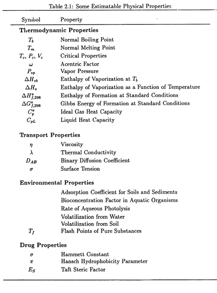
Estimation techniques are available for thermodynamic properties[lOl], enVIron-ment.al propcrties[79], and polymer properties[127]. Estimating biological activity is the major thrust of (lrug design[39,53,84]. Table 2.1 presents a brief list of physical properties whose vall1es can be estimated.

l\·rany approaches are taken to relate molecular structure to physical properties. I classify physical property estimation techniques iIlto five categories:

1. pattern recognition

2.

topological

3.

group contribution

4.

equation oriented 5. molecular modeling

I l>riefly describe each of these categories in the following sections. Each section contains a short discussion of the con.cepts Ilsed followed by an example.

2.1.1 Pattern Recognition

Pattern recognition techniques are often employed when causal relationships are not \vell uneJerstood. Discriminant analysis and classification are two statistical techniques used in pattern recognition. Both aremultivariatetechniques concerned with separatin,g

distinct sets of objects intoclasses and with allocating newobjects to previously defined classes. Discriminant analysis develops a discriminant function which classifies new compounds based on their molecular features. In many applications the number of classes equals t\vo: carcinogenic or noncarcinogenic; toxic or nontoxic; etc.

Discriminant analysis begins with a set of observations and a desire to separate them into two or more classes. Each observation has a set of "features" used in the

(33)

I

Synlbol

Table 2.1: Some Estimatable Physical Properties Property

Tllermodynamic Properties

Tb

T

m

T

c ,

Pc, Vc

w PVP ~Hvb ~Hv ~HJ,298 LlGj,298

Co

P CpL

Normal Boiling Point Normal rvlelting Point Critical Properties Acentric Factor Vapor Pressure

Enthalpy of Vaporization at Tb

Enthalpy of Vaporization as a Function of Temperature Enthalpy of Formation at Standard Conditions

Gibbs Energy of Formation at Standard Conditions Ideal Gas Heat Capacity

Liquid Heat Capacity

Transport Properties

17 Viscosity

A

Thermal Conductivity DAB Binary Diffusion Coefficient

(j Surface Tension

Environmental Properties

Adsorption Coefficient for Soils and Sediments Bioconcentration Factor in Aquatic Organisms Rate of Aqueous Photolysis

'volatilization from Water Volatilization from Soil

T

_J Flash Points of Pure Substances

Drug Properties

u Hammett Constant

1r Hansch Hydrophobicity Parameter

(34)

Table 2.1 Continued: Some Estimatable Physical Properties

S)rmbol

Property

Pol~,merProperties

Tg

Glass Transition Temperature

T

m Crystalline Melting Temperature

(} Thermal Expansion Coefficient f Dielectric Constant

X Magnetic Susceptibility

B

Specific Bulk Morlulus

classification. The objective of the analysis is to develop a discriminant function which given the features of an observation correctly classifies the compound. A subset of compoun<ls, called the "training set", is tlsed to develop the discriminant function. Once the discriminant function is formed it is used for classifying new observations.

De,'eloping a discriminant function begins by separating our training observations into separate classes. For two classes, 1rl and 1r2, we obtain two collections of

p-dimensional feature vectors: ~Y'1 and

X

2 •

A

discriminant function is then developed

whicll

optimally

classifies

..,l[l into 1rl and J1[2 into 1r2. We assume this function is linear

of the form:

n

y=L,ljxj

i=1

(2.1)

\Vllere

Ij

is tIle

loading

of

each feature and y is a flew variable called a

discriminant

val-jable. The analysis thus transforms a multiva,riate observation on X into a univariate observation on y.

(35)

7 6 5 I'

6/~2'

5'

0

3' 4' HN 9 4 2 3

Figure 2.1: General Structure of 9-Anilinoacridine

we form the allocation rule:

If

Then

Else

Y·J -

>m

Allocate observation j having feature vector Xj to class 1l"t. Allocate observation j having feature vector Xj to class

1r2-An important part ofdetermining theclassification function istoidentify which fea-tures are important for classification. Additionally determining the minimtlffi number of features facilitates theoretical interpretation of the results.

Henry, et.al.[55] performed a pattern recognition study of the antitumor activity of a set of 9-anilinoacridines. The general structure of the set of molecules is shown in Figure 2.1. Four classes ofdescriptors were used to separate the compounds into active and inactive classes. The four classes were:

l~ Fragment descriptors - various atom, bond, and ring counts and molecular weight. 2. Topological descriptors: various X indices.

3. Substructure environment desc~iptors: the presence or absence of specific molec-ular substructures. Table 2.2 lists thesesubstructures.

(36)

Table 2.2: Specific Substructure Descriptors 1) X-NH2

9)

2>-

NH-@-NH-S0

2-X

X

2)

X-CH₂-CH₃ 3)

X-(ClI

_2)3-

X

10)

Y

2>-

NH

2

4)

NH

X

0

II 5) X-C-NHi

0 II

HN-@-

X 6)

X-C-NH-X

11)

X-NH-@-NH-X

7)

8)

x - @ - NH-S0

2

-X

*

denotes an unspecified substituent.

4. Physicochemical property descriptors: Bondi'5 molecular volume[11], molar

re-fractivity, the del-Re (J' electronic charges at various positions on the aniline anacridine rings[25], and logP.

A set of 18 descriptors were obtained which could correctly classify 94% of the com-pOUDcls in the training set of 213. 97% of the active compounds and 85% of the inactive compounds \vere correctly classified. These descriptors appear in Table 2.3.

TIle

weight vector that was obtained from the training set was applied to a pre-diction set of 119 compounds that were not included in the original analysis. The prediction set results had an accuracy greater than 73% indicating the usefulness of

(37)

Table 2.3: 18 Descriptors for Antitumor Activity Classification

Descriptor Coefficient Variance

1)

#

of

S

atoms

0.169

0.012 2)

#

of rings

-0.172

0.002

3)

Average

#

of 0.326 0.004

paths per atom

4)

Molar Refractivity -0.213

0.010

5) Substructure 1 -0.141 0.011

6)

Substructure 2 0.033 0.044

7)

Substructure 3 0.090 0.029

8)

Substructure 4

0.457

0.003

9)

Substructure 5 0.083 0.027 10) Substructure 6 -0.129 0.017

11)

Substructure 7

0.224

0.003 12) Substructure 8 0~086

0.061

13) Substructure 9 -0.323 0.002 14) Substructure 10

-0.241

0.017 15) Substructure 11

-0.128

0.004

16) Charge Position 2

-0.142

0.016 17) Charge Position 3 0.153 0.001 18) Charge Position 2' -0.333 0.018 Constant

0.361

0.003

(38)

pattern recognition in screening active compounds.

2.1.2 Topological Techniques

Topological tecllniques ignore the actual three-dimensional shape of a molecule, the nature and lengths of the chemical bonds connecting its atoms, the angles between tIle bonds, and sometimes even atom types[107].

Only

the number of atoms and their interconnections are considered. This information is reduced to an index. Some of the proposed indices are the \Viener Path Number[132], Alternburg Polynomial Index[2], Gordon and Scantlebury Index[46] , Hosoya's Z Index[59], and Randic's Branching Index[96]. Randic's in:lex has been formalized and extended by Kier and Hall[65]. I use the extension of

Randic's

index

by

Kier

and

Hall to demonstrate this class of estimation techniques.

Calculation of the index begins by drawing a hydrogen suppressed molecular graph. The graph for 2,2-dimethylbutane is:

1

4

1 1

2

1 The numbers

correspond

to a

valence,

6,

assigned

to each

carbon atom equal to the number of C-C bonds in which the atom participates. Using the Randicalgorithm the contribution of each bortd toward the index is:

(2.2)

(39)

x.

For 2,2-dimethylbtltane:

1 1 1 1 1

X=

+

-f.

+

=

2.5607

yT:4

J4:2

J2:T

!(ier and

Hall

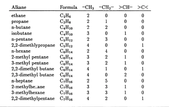
extended the algorithm to include heteroatoms[65].

Table

2.4

showsXana Tbvalues for 39 alkanes. Linearregressionoft.he data resulted

in the equation

Tb

=

67.5X - 130.0

llaving an r2 value of 0.977.

2.1.3 Group Contribution Techniques

(2.3)

Group contribution techniques make the assumption that each fragment of a molecule contributes a certain amount to the value of its physical property. The further

assurnp-tioD

is made that this contribution is dependent only upon the local conditions, the atom itself, its neighbors, and sometimes its neighbors neighbors.

Developing group contribution techniques begins by collecting a set of molecules having known values for the property to be estimated. A set of grvups is chosen wllich can represent the molecules. The occurrenceof these groups in each molecule is recorded.

Taking data for the Gibbs energy of formation for the alkanes we obtain the following four groups:

>CH-

>c<

(40)

Alkane

Table 2.4: X and TbData for Alkanes

x

Ethane Propane n-Butane 2-~Ietllylpropane n-Pentane 2-Methylbutane 2,2-Dimethylpropane n-Hexane 2- Methylpentane 3- Methylpentane 2,2-Dimethylbutane 2,3-Dimethylbutane n-Heptane 2-Methylhexane

3-

Methylhexane 3-Ethylpentane 2,2-Dimethylpentane 2,3-Dimethylpentane 2,4-Dirnethylpentane 3,3-Dimethylpentane 2,2,3-Trimethylbutane n-Octane 2-Methylheptane

3-

Methylheptane 4-Methylheptane 3-Ethylhexane 2,2-Dimethylhexane 2,3-Dirnethylhexane 2,4- Dimethylhexane

2,5-

Dimethylhexane 3,3-Dimethylhexane

3,4-

Dimethylhexane

2-Methyl-3-Ethylpentane

3-Methyl-3-Ethylpentane 2,2,3-Trimethylpentane 2,2,4-Trirnethylpentane 2,3,3-Trimethylpentane

2,3,4-

Trirnethylpentane 2,2,3,3-Tetramethylbutane 1.00000 1.41421 1.91421 1.73205 2.41421 2.27005 2.00000 2.91421 2.77005 2.80806 2.56066 2.64273 3.41421 3.27005 3.30806 3.34606 3.06066 3.18073 3.12589 3.12132 2.94337 3.91421 3.77005 3.80806 3.80806 3.84606 3.56066 3.68073 3.66390 3.62589 3.62132 3.71784

3.71784

3.68198 3.48138

3.41650

3.50403 3.55341 3.25000

-88.630

4H1O

3

0

1 0 n-pentane CSH12 2 3 0 0 2,2-dimethlypropane

C

SH12 4

0

0 1 n-hexane

C6

Ht4

2 4 0 0 2-methyl pentane

C6

n-heptane

C

7

H

16

2

5

0

2-methylhe:~ane C1H16 3 3 1 0 3- methylhexane C7H16 3 3 1 0 2,2-dimethylpentane C7H16 4 2

0

1

For n compounds our data consists of an

(n

xl)

vector of physical properties, P, al1d an (n x

4)

matrix of group occurrences, G. Assuming a linear relationship between tIle occurrences of the groups and the physical property we formulate the problem as

finding the vector of4 group contributions,

a,

such that

Ga=P

(2.4)

Eqllation 2.4 is overdetermined and is solved using a regression technique. The most

commonly used regression is least squares giving

(2.5)

Data from 54 alkanes were regressed onto our four groups. The resulting m.odel of the regression is

(42)

Table 2.6: LlG/₁₂₉₈ Group Contribution Estimation Errors

Compound Formula Literature Error

6H14 -0.06

H

34 20.00 0.16

Error

=

Estimat.e - Literature. Units are kJ/mol. Literature values were from [101].

TIle7.2 value was 0.975. Table 2.6 shows theerrors ofthe estimation for 20 compounds.

Group contribution estimation techniques

can

become very complex

including

non-linear effects and interactions among groups. UNIFAC[41] is an example of a complex group contribution estimation technique.

2.1.4 Equation Oriented Techniques

Equation oriented estimation techniques are the most widely used type of estimation tecllnique. One physical property is related to one or more other pllysical properties by

(43)

tllcoretical or empirical models~ The goal is to relate the estimated physical properties to properties more available or more easily measured.

Eqtlation oriented estimation techniques are typically a combination of theory and empiriczl observation. Theoretical concepts often suggest interrelations among physical properties or between properties and state variables_ These premises instigate empirical inquiry into reifying such relationships.

Klincewicz[67] developed an equation oriented estimation technique for the critical temperature.

Tc

is related to

T

b and l~fw by

Tc

=

50.2 - O.16Mw

+

1.41Tb

(2.7)

Table 2.7 shows the errors associated with estimating 20 compounds. Errors of between 1 to 2 percent were reported[102]. Using Equation 2.7 I estimated

Tc

for 406 organic compounds obtaining an average absolute error of 18.7 K giving an average absolute percent error of 3.1

%.

2,,1.5

Molecular Modeling

Techniques

The ultimate objecti\t"e of a molecular approach to physical properties is to calculate tIle macroscopic properties of matter from first principles. The term "first principles" refers to quantum theory and to statistical mechanics. The mathematical solution

of the formulas of quantum mechanics provides us with the microscopic or molecular energy values, anyone of which a systemmay assume at a given instant of time. With the microscopic energy levels available, the methods of statistical mechanics can be applied to give the observable or blilk properties of the molecular system.

(44)

Table 2.7:

T

c Equation Oriented Estimation Technique Errors

Compound Formliia Tc Error

%

C

2

H

3

N

545.5

-1.6 -0.3 Acetic Acid C2H402 592.7

-0.7

-0.1 Ethane

C

2

H

s 305.4

0.3

0.1 Glycerol

C

3Hs

0

3 726.0 103.3 14.2

rvlethyl Ethyl Sulfide

C

3Hs

S

533.0

-15.9

Bulk

properties ofsystem

The objective of statistical mechanics is to show how the properties of matter in bulk (Inacroscopic properties) can be calculated from the properties of individual molecules (positions, molecular geometry, interatomic and intermolecular forces, etc.). Quantum mechanics alone cannot sllpply these macroscopic properties because it deals with the detailed dynamics of the particles.

The whole field of molecular mechanics, conformational energy calculations, and molecular dynamics simulations rests on the fact that the potential energy of a mole-cule or assembly of mole~ulescan be written as an analytically simple sum of terms, involving internal coordinates of the molecule (i.e., bond lengths, bond angles, torsion angles, and interatomic distances )[48]. This potential energy function is a fundamental physical quantity, implicitly containing essentially all conformational properties of the molecular system

CJf

interest (with theexceptionof quantumproperties). Some of these properties are presented in Table 2.8.

Molecular dYllamics can be used to compute the dynamics of the molecular system. The first step is specifying the potential energy expression. Initial coordinates and velocities are specified for each of the atoms in the system. Once tIle initial conditions are specified, the equations of motion:

_ av _

F _

m. £Prj

(46)

Table 2.8: Properties Available from the Potential Energy }iunction

v

aV/8x

=

0 -8V/8x

=

F

=

rna

Energy

Monte Carlo solvent effects Minimum-energy conformation Vibrational spectra

Normal modes

Entropy and free energy Dynamic trajectory

Conformational fluctuations

are written for each atom. The equations are then integrated forward in time to com-pllte the trajectories of each atom.

2.2 Selecting Chemical Products

Selecting existing compounds for use as chemical products is a two step procedure. TIle first step involves identifying those physical properties which are important to the performance of the chemical product and their values which give optimal behavior. The second step is searching a data base for existing compounds possessing these physical property values.

Identifying important physical properties is not a triv~ial task. Thermodynamic, transport, environmental, and economic factors must be accounted for in making deci-sions. The procedures used for solvent selection exemplify the multiple ways in which the problem can be formulated. Three solvent selection procedures are discussed.

(47)

Table 2.9: Godfrey's Standard Solvents and Miscibility Number 1 Glycerol 2 Ethylene Glycol

3

1,4-Butanediol

4 2,2'-

Thiodiethanol 5 Diethylene Glycol 6 Triethylene Glycol 7 Tetraethylene Glycol

8

Methoxyacetic Acid 9 Dimethyl Sulfoxide

10

N-Formylrnorpholine 11 Furfuryl Alcohol 12 2-(2-Methoxyethyoxy) Ethanol 13 2-Methoxyethanol 14 2-Ethoxyethanol

15

2-(2-Butoxyethoxy) Ethanol 16 2-Butoxyethanol

- 2.2.1

Godfrey

17 p-Dioxane 18 3-Pentanone 19 1,1,2,2-Tetrachloroethane 20 1,2-Dichloroethane 21 Chlorobenzene 22 1,2-Dibromobutane 23 I-Bromobutane 24 I-Bromo-3-methylbutane 25 sec-Amylbenzene

26 4-

Vinylcyclohexane 27 I-Methylcyclohexene 28 Cyclohexane 29 Heptane 30 Tetradecane 31 Petrolatum

Godfrey[44] addressed the problem of identifying whether 01' not two liquids were

mis-cible. He selected 31 typical solvents which spanned the range from strongly lipophilic to strongly lipophobic:. To each of these solvents he assigned a

Miscibility

Number.

Table 2.9 shows the 31 solvents with their assigned miscibility numbers.

Godfrey developed

th.e following

three rules to determine miscibility of two liquids:

1. All pairs of standard solvents whose miscibility numbers differ by 15 or less are miscible in all proportions at 25°C.

2. Each pair whose miscibility number difference is 16 has a critical solution tem-perature between 25° and 75°C.

(48)

temperature above 75°C.

To classify a new liquid in the miscibility number system, the chemist determines a cut-off in miscibilityor immiscibility vlith the standard solvents. 15 is then added or subtracted to the miscibility number of the standard to give the new solvent'8 number.

In this manner Godfrey determined the miscibility number for over400organic liquids.

2.2.2 Francis

Francis[38] developed a solvent selection procedure emphasizing selectivity for hydro-carbons. He investigated the applicability of critical solution theory as a measure of affinity. The temperature at which a liquid mixture separates into its components is its critical solution temperature.

Figure 2.2 shows the solubility behavior of three hydrocarbons in aniline. The three hydrocarbons boil almost at the same temperature, so they can not be readily separated by fractional distillation. In solvent' extraction the hydrocarbons form approximately ideal mixtures, so that the amounts extracted

by

a solvent are nearly proportional to the separate solubilities. Since the three curves have almost exactly the same shape except for vertical displacement, the solubilities are related simply to the critical solution temperature.

2.2.3 Berg

Berg[8]

developed

a

classification scheme for hydrogen bonding in azeotropic distillation solvents. Five classes of solvents were formed ranging from highly hydrogen bonding

(49)

80 - X X X 0 0 0 0 0 0 60 - x₀ ~ 0 X 0 0 ... XO I-40 -

_·0

D X 0

Xo

c 20 -

_'b

c D Methylcyclohexane )I) c ₀ n-Heptane Xo D X iso-Octane

.

_D 0 I I I I 0 10 20 30 40 50 okHydrocarbonbyWeight

Figure 2.2: Critical Solution Temperatures of Three Liquid Mixtures

substances to non-hydrogen bonding substances. The classes are listed here:

• Class I: Liquids capable of forming three dimensional networks of strong hydro-gen bonds - e.g.; water, glycol, glycerol, amino alcohols, hydroxylamine, hydroxy-acids, polyphenols, amides, etc.

• Class II: Other liquids composed of molecules containing both active hydrogen atoms and donor atoms (oxygen, nitrogen, and fluorine) - e.g.; alcohols, acids, phenols, primary and secondary amines, nitro compounds with alpha-hydrogen atoms, nitriles with alpha-hydrogen atoms, anlffionia, hydrazine, hydrogen fluo-ride, hydrogen cyanide, etc.

• Class III: Liquids composed of molecules containing donor atoms but no active hydrogen atoms - e.g.; ethers, ketones, aldehydes, esters, tertiary amines, nitro

(50)

compounds, etc.

• Class IV: Liquids composed of molecules containing active hydrogen atoms but no donor atoms. These are molecules having two or three chlorine atoms on the same carbon atoms as a hydrogen atom, or one chlorine on the same carbon atom and one or more chlorine atonlS on adjacent carbon atoms - e.g.; CHCI3 , CH2C12 ,

• Class V: All other liquids - i.e., liquids having no hydrogen bond forming capa·· bilities - e.g.; hydrocarbons, CS2 , sulfides, mercaptans, halohydrocarbons, etc.

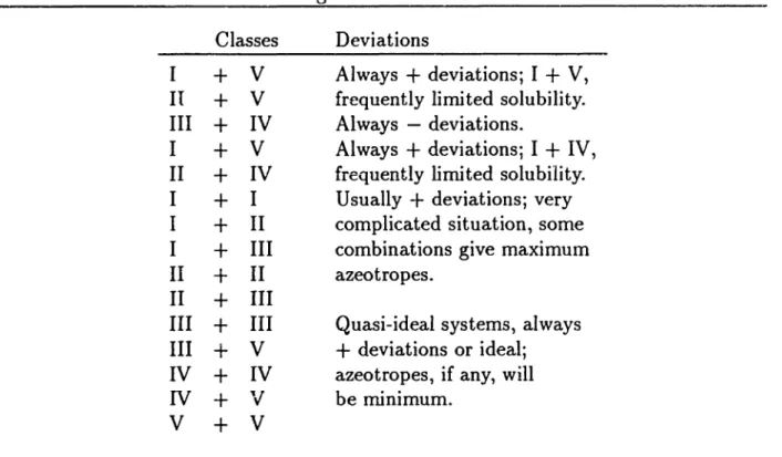
Table 2.10 shows the ordering of deviations from Raoult's law. Berg proposed this ranking to assist identifying solvents for use in azeotropic distillation. To form an azeot.rope with a compound from Class I Table 2.10 suggests examining compounds in Class

v.

2.3 Designing Chemical Products

Designing new chemical products is a two step approach similar to that used in selecting chemicalproducts. The first step is identical:

identify

the importantphysical properties and tlleir values. The second step is to search for compounds which possess acceptable values for these important physical properties. However, unlike selecting from existing compounds, we do not ha""e a data base of existing compounds to search. The molecular structures of new compounds must be h)'pothesized.

(51)

Table 2.10: Ordering of Deviations from Raoult's Law Classes

I

+

V

II

+

V

III

+

IV

I

+

V

II

+

IV I

+

I

+

IV

+

IV IV

+

'v

V

+

V Deviations Always

+

deviations; I

+

V, frequently limited solubility. Always - deviations.

Always

+

deviations; I

+

IV, frequently limited solubility. Usually -t- deviations; very complicated situation, some combinations give maximum azeotropes.

Quasi-ideal systems, always

+

deviations or ideal; azeotropes, if any, will be minimum.

never been synthesized, physical propertyestimation techniques play an important role in chemical product design. The three techniques discussed here form candidate mol-ecules and estimate their properties using estimation techniques. Grollp contriblltion estimation techniques are used in all three cases.

2.3.1 Solvent Desigll

Gani and Brignole

[13,42]

used the UNIFAC[41] group contribution method to synthe-size molecularstructures with specific solvent properties for the separation of aromatic and paraffinic hydrocarbons by liquid-liquid extraction. Their synthesis procedure is di\rided into 3 steps:

1. Select the group3 considered suitable building blocks for the molecular structures. 2. Combine the groups into candidate molecules according to specified combination

(52)

Table 2.11: Groups Used in Solvent Design

-CH

₃

-(C

S

H

4

N)

-OCH3 -CH 2--CH₂ CO-CH3

COO--COCH

₃ >CHN02 -CH2

COO--CH2CN

-(C

S

H

3

N)--CH₂

0-3. Screen the candidate molecules using UNIFAC to evaluate their usefulness for a particular solvent extraction task.

Chlorinated, olefinic, carboxylic, aldehyde, and aromatic groups were excluded from the design because of potential chemical instability or corrosion problems. Table 2.11

SllO\VS tile resulting fourteen groups used in the design.

To reduce the number of group combinations to a tractable number several addi-tional constraints were placed on the candidate solvents. The solvents should have a rather high boiling point to obtain a simple separation from the aromatic fraction and to avoid the formation of azeotropes. This constraint on the boiling point was propagated to a constraint Ofl the minimum vallIe for molecular weight being 100. A

nlaxirnum valuewas chosen to be 140. Another constraint was that a candidate solvent should have at

least

one nonhydrogen group.

In one analysis 85 compounds were obtained after screening according to chosen grOtlpS, structural constraints, and molecular weight range. These were tested using UNIFAC

for

their use as a solvent for the separation of n-heptane and toluene. Fourteen compounds were found to have satisfactory solvent properties.

(53)

Table 2.12: Groups used in Polymer Design

2.3.2 PolYll1er

Design

-co- -CONH-

-CHCI-

-coo-

-CHOH-Derringer and Markham[26] proposed a generate and test methodology for designing polymers possessing desired physical properties. They based their methodology upon J<revelen's[127] group contribution estimation techniques. A computer program was \vritten to find viable polymer structures for meeting constraints on three physical properties:

1. density, D

2. water absorption, W

3. glass transitioIl temperature,

Tg •

Tile groups comprising the repeat unit were limited to the seven shown in Table 2.12. Van Krevelen described estimation models for the three physical properties:

Tg -

(L

~i

/L

M; ) - 273°C

;.\/; is the contribution of the ith group to the gram molecular weight, ~i the con-tribution to the molar volume,

Hi

the contribution to the molar \vater content, and

~i the contribution to the molar glass transition temperatl1re function. The group contributions are given in Table 2.13.

(54)

Table 2.13: Group Contributions used in Polymer Design Group

M

j ~i

Hi

~i -CH2- 2,700 15.85 3.3xlO-s 14.0

-CO-

the computer program generated 300 candidate polymers randomly selecting both the number of groups per structural repeat unit and the groups themselves. Only 12 of tllese candidates satisfied the target specifications. These are shown in Table 2.14.

Recognizing that the number of candidates which are identified may be large, Der-ringer and Markham devised a ranking procedure. This procedure:onsists of the following two steps:

Designing molecules possessing desired physical property values

Designing IVlolecules Possessing Desired Physical

G.

©

©

by

_

OCT 3

1989

wI. Deen

Abstract

Problem Formulation:

2. Target Transformation:

3. Group Selection:

4. Molecule Enumeration:

of

5. Molecule Screening:

6. Final

Contents

...

1.2

...

6

2.1.1

..

16

2.1.5

2.2

2.2.1

24

2.2.2

25

2.2.3

..

25

2.3

....

27

28

2.3.2

2.3.3

2.3.4

2.5

DENDRAL

. .

.

· ....

2.6

49

3.2

52

3.3

52

3.4

....

...

· ....

· .

4.2

4.2.1

· ....

66

4.3

4.4

.

.

....

70

....

4.4.2

·

...

...

71

4.4.3

72

4.5

...

Target Transformation

5.2

_{· .}

_{· ....}