Development of a model to predict flow oscillations in low-flow sodium boiling

Alan E. Levin Peter Griffith

Energy Laboratory Report No. MIT-EL-80-006 April 1980

MITLibraries

Document Services Email: docs@mit.edu_{http://Iibraries.mit.edu/docs}

DISCLAIMER OF QUALITY

Due to the condition of the original material, there are unavoidable

flaws in this reproduction. We have made every effort possible to

provide you with the best copy available. If you are dissatisfied with

this product and find it unusable, please contact Document Services as

soon as possible.

Thank you.

Some pages in the original document contain pictures,

graphics, or text that is illegible.

A. Topical Reports (For availability check Energy Laboratory Headquarters, Room E19-439, MIT, Cambridge, Massachusetts, 02139)

A.1 General Applications

A.2 PWR Applications A.3 BWR Applications A.4 LMFBR Applications

A.1 M. Massoud, "A Condensed Review of Nuclear Reactor

Thermal-Hydraulic Computer Codes for Two-Phase Flow Analysis," MIT Energy Laboratory Report MIT-EL-79-018, February 1979.

J.E. Kelly and M.S. Kazimi, "Development and Testing of the Three Dimensional, Two-Fluid Code THERMIT for LWR Core and Subchannel Applications," MIT Energy Laboratory Report MIT-EL-79-046, December 1979.

A.2 P. Moreno, C. Chiu, R. Bowring, E. Khan, J. Liu, N. Todreas, "Methods for Steady-State Thermal/Hydraulic Analysis of PWR Cores," MIT Energy Laboratory Report MIT-EL-76-006, Rev. 1, July 1977 (Orig. 3/77).

J.E. Kelly, J. Loomis, L. Wolf, "LWR Core Thermal-Hydraulic Analysis--Assessment and Comparison of the Range of Applica-bility of the Codes COBRA-IIIC/MIT and COBRA IV-l," MIT

Energy Laboratory Report MIT-EL-78-026, September 1978. J. Liu, N. Todreas, "Transient Thermal Analysis of PWR's by a Single Pass Procedure Using a Simplified Model Layout," MIT Energy Laboratory Report MIT-EL-77-008, Final, February 1979,

(Draft, June 1977).

J. Liu, N. Todreas, "The Comparison of Available Data on PWR Assembly Thermal Behavior with Analytic Predictions," MIT

Energy Laboratory Report MIT-EL-77-009, Final, February 1979, (Draft, June 1977).

A.3 L. Guillebaud, A. Levin, W. Boyd, A. Faya, L. Wolf, "WOSUB-A Subchannel Code for Steady-State and Transient

Thermal-Hydraulic Analysis of Boiling Water Reactor Fuel Bundles," Vol. II, Users Manual, MIT-EL-78-024. July 1977.

L. Wolf, A Faya, A. Levin, W. Boyd, L. Guillebaud, "WOSUB-A Subchannel Code for Steady-State and Transient

Thermal-Hydraulic Analysis of Boiling Water Reactor Fuel Pin Bundles," Vol. III, Assessment and Comparison, MIT-EL-78-025, October 1977-.

L. Wolf, A. Faya, A. Levin, L. Guillebaud, "WOSUB-A Subchannel Code for Steady-State Reactor Fuel Pin Bundles," Vol. I, Model Description, MIT-EL-78-023, September 1978.

A. Faya, L. Wolf and N. Todreas, "Development of a Method for BWR Subchannel Analysis," MIT-EL-79-027, November 1979.

A. Faya, L. Wolf and N. Todreas, "CANAL User's Manual," MIT-EL-79-028, November 1979.

A.4 W.D. Hinkle, "Water Tests for Determining Post-Voiding Behavior in the LMFBR," MIT Energy Laboratory Report MIT-EL-76-005,

June 1976.

W.D. Hinkle, Ed., "LMFBR Safety and Sodium Boiling - A State of the Art Reprot," Draft DOE Report, June 1978.

M.R. Granziera, P. Griffith, W.D. Hinkle, M.S. Kazimi, A. Levin, M. Manahan, A. Schor, N. Todreas, G. Wilson, "Development of Computer Code for Multi-dimensional Analysis of Sodium Voiding in the LMFBR," Preliminary Draft Report, July 1979.

M. Granziera, P. Griffith, W. Hinkle (ed.), M. Kazimi, A. Levin, M. Manahan, A. Schor, N. Todreas, R. Vilim, G. Wilson, "Develop-ment of Computer Code Models for Analysis of Subassembly Voiding in the LMFBR," Interim Report of the MIT Sodium Boiling Project Covering Work Through September 30, 1979, MIT-EL-80-005.

A. Levin and P. Griffith, "Development of a Model to Predict Flow Oscillations in Low-Flow Sodium Boiling," MIT-EL-80-006, April 1980.

M.R. Granziera and M. Kazimi, "A Two Dimensional, Two Fluid Model for Sodium Boiling in LMFBR Assemblies," MIT-EL-80-011, May 1980.

G. Wilson and M. Kazimi, "Development of Models for the Sodium Version of the Two-Phase Three Dimensional Thermal Hydraulics Code THERMIT," MIT-EL-80-010, May 1980.

B.1 General Applications B.2 PWR Applications B.3 BWR Applications B.4 LMFBR Applications

B.1 J.E. Kelly and M.S. Kazimi, "Development of the Two-Fluid Multi-Dimensional Code THERMIT for LWR Analysis," accepted

for presentation 19th National Heat Transfer Conference, Orlando, Florida, August 1980.

J.E. Kelly and M.S. Kazimi, "THERMIT, A Three-Dimensional, Two-Fluid Code for LWR Transient Analysis," accepted for presentation at Summer Annual American Nuclear Society Meeting, Las Vegas, Nevada, June 1980.

B.2 P. Moreno, J. Kiu, E. Khan, N. Todreas, "Steady State Thermal Analysis of PWR's by a Single Pass Procddure Using a

Simpli-fied Method," American Nuclear Society Transactions, Vol. 26 P. Moreno, J. Liu, E. Khan, N. Todreas, "Steady-State Thermal Analysis of PWR's by a Single Pass Procedure Using a Simplified Nodal Layout," Nuclear Engineering and Design, Vol. 47, 1978, pp. 35-48.

C. Chiu, P. Moreno, R. Bowring, N. Todreas, "Enthalpy Transfer Between PWR Fuel Assemblies in Analysis by the Lumped Sub-channel Model," Nuclear Engineering and Design, Vol. 53, 1979,

165-186.

B.3 L. Wolf and A. Faya, "A BWR Subchannel Code with Drift Flux and Vapor Diffusion Transport," American Nuclear Society Transactions, Vol. 28, 1978, p. 553.

B.4 W.D. Hinkle, (MIT), P.M Tschamper (GE), M.H. Fontana, (ORNL), R.E. Henry (ANL), and A. Padilla, (HEDL), for U.S. Department of Energy, "LMFBR Safety & Sodium Boiling," paper presented at the ENS/ANS International Topical Meeting on Nuclear Reactor Safety, October 16-19, 1978, Brussels, Belgium.

M.I. Autruffe, G.J. Wilson, B. Stewart and M. Kazimi, "A Pro-posed Momentum Exchange Coefficient for Two-Phase Modeling of Sodium Boiling," Proc. Int. Meeting Fast Reactor Safety Tech-nology, Vol. 4, 2512-2521, Seattle, Washington, August 1979. M.R. Granziera and M.S. Kazimi, "NATOF-2D: A Two Dimensional

Two-Fluid Model for Sodium Flow Transient Analysis," Trans. ANS, 33, 515, November 1979.

This report was prepared as an account of work sponsored by the United States Government and two of its subcontractors. Neither the United States nor the United States Department of Energy, nor any of their employees, nor any of their con-tractors, subconcon-tractors, or their employees,

makes any warranty, express or implied, or assumes any legal liability or responsibility for the

accuracy, completeness or usefulness of any information, apparatus, product or process dis-closed, or represents that its use would not infringe privately owned rights.

by

Alan E. Levin Peter Griffith

Energy Laboratory,

Department of Nuclear Engineering and Department of Mechanical Engineering Massachusetts Institute of Technology

Cambridge, Massachusetts 02139

Topical Report of the MIT Sodium Boiling Project

sponsored by

U. S. Department of Energy, General Electric Co. and

Hanford Engineering Development Laboratory

Energy Laboratory Report No. MIT-EL-80-006

ABSTRACT

An experimental and analytical program has been carried out in order to better understand the cause and effect of flow

oscillations in boiling sodium systems. These oscillations

have been noted in previous experiments with liquid sodium, and play an important part in providing cooling during Loss-of-Piping Integrity (LOPI) accidents that have been postulated

for the Liquid Metal-Cooled Fast Breeder Reactor.

The experimental program involved tests performed in a

small scale water loop. These experiments showed that voiding

oscillations, similar to those observed in sodium, were present

in water, as well. An analytical model, appropriate for either

sodium or water, was developed and used to describe the water flow behavior.

The results of the experimental program indicate that water can be successfully employed as a sodium simulant, and further, that the condensation heat transfer coefficient varies signifi-cantly during the growth andcollapse of vapor slugs during

oscil-lations. It is this variation, combined with the temperature

profile of the unheated zone above the heat source, which deter-mines the oscillatory behavior of the system.

The analytical program has produced a model which quali-tatively does a good job in predicting the flow behavior in the

wake experiment. Quantitatively, there are some discrepancies

between the predicted and observed amplitudes of the oscillations. These discrepancies are attributable both to uncertainties in the experimental measurements and inadequacies in modelling the

several parameters, including the heat transfer coefficient, unheated zone temperature profile, and amount of mixing

be-tween hot and cold fluids during oscillations, are set by the user, and have a deterministic effect on the behavior of the model.

Additionally, criteria for the comparison of water and sodium experiments have been developed. These criteria have not been fully tested.

Several recommendations for future study are proposed, in order to advance the capability of modelling the phenomena observed.

ACKNOWLEDGEMENT

Funding for this project was provided by the United States Department of Energy, the General Electric Co., and the Hanford Engineering Development Laboratory. This support was deeply appreciated.

The authors also thank Dr. William Hinkle and Prof. Neil Todreas for their helpful suggestions, Messrs. Joseph Caloggero and Fred Johnson for their help in acquiring materials for and constructing the Water Test Loop, and Messrs. Chris Mulcahy and Lee Shermelhorn for their help with the data acquisition

system.

The work described in this report was performed primarily by the principal author, Alan E. Levin, who has submitted the

same report in partial fulfillment for the ScD degree in Nuclear Engineering at MIT.

TABLE OF CONTENTS PAGE Title Page . . . . 3 Abstract . . . . . . . . . . ... 4 Acknowledgements . . . . 6 Table of Contents . . . . 7 List of Figures . . . ... * . 12 List of Tables . . . . 15 Nomenclature . . . . . . . . . . .. . *... . 16 CHAPTER 1: INTRODUCTION . . . . 20 1.1 Background . . . . 20

1.2 Scope of the Work . . . . 22

CHAPTER 2: THE ANALYTICAL MODEL . . . . . . . . . 27

2.1 Overall Concept . . . . 27

2.2 The Hydrodynamic Model . . . . . . . . . . 28

2.3 The Thermal Model . . . . 33

2.4 Solution of the Equations . . . . 36

2.5 Limitations of the Model . . . . . . . . . 41

CHAPTER 3: CRITERIA FOR THE COMPARISON OF BOILING SODIUM TO WATER . . . . . 43

3.1 Background . . . . 43

3.2 Momentum Equations . . . . 45

3.3 The Compressibility Equation . . . . . . . 47

TABLE OF CONTENTS (Cont.)

3.5 Comparison of Sodium Data to Water Data . . .

PAGE

52

CHAPTER 4: EXPERIMENTAL APPARATUS AND

PROCEDURES . . . . . . . . . . . . .

4.1 Background and Experimental Apparatus .

4.2 Experimental Set-up and Procedure ...

4.2.1 Pretest Set-up and Calibration . . .

4.2.2 Experimental Procedure . . . . . . .

4.2.2.1 Stagnant Flow Tests . . . . . .

4.2.2.2 Forced Convection Testing . . .

4.3 Safety Precautions . . . . . . . . . . .

CHAPTER 5: EXPERIMENTAL AND ANALYTICAL RESULTS.

. . 53 . . 53 . 62 . 62 . 64 . 64 . 67 . . 68 . . 70 5.1 Experimental Results . . . . . . . . . . . . 70

5.1.1 Stagnant Flow Tests . . . . . . . . . . 70

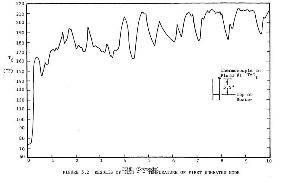
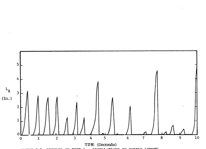
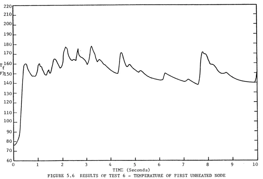
5.1.1.1 Data Analysis . . . . 70 5.1.1.2 Test 4 . . . . 73 5.1.1.3 Test 5 . . . . 77 5.1.1.4 Test 6 . . . . 81 5.1.1.5 Test 7 . . . . 85 5.1.1.6 Tests 8 and 9 . . . . 85

5.1.2 Forced Convection Testing . . . . . . . 92

5.1.3 Sources of Error and Uncertainties

TABLE OF CONTENTS (Cont.)

PAGE

5.1.3.1 Stagnant Flow Tests . . . . . . . 95

5.1.3.2 Forced Convection Testing . . . . 96

5.1.3.3 Other Sources of Error ... 97

5.1.4 Calculation of Condensation Heat Transfer Coefficient . . . . . . . .. 98

5.1.5 Comparison of Water Data to Sodium Data . . . . . . . . . . . . . 101

5.2 Analytical Results . . . . . . . . . . . . 103

5.2.1 Features of Analytical Simulations . . 104

5.2.2 Comparison of Analytical and Experi- 114 mental Test Results . . . . . . . . . CHAPTER 6: CONCLUSIONS AND RECOMMENDATIONS FOR FUTURE STUDY . . . . . . . . . . . . . 131

6.1 Conclusions . ... ... 131

6.2 Recommendations for Future Work . . . . . . 132

REFERENCES . . . . 135

APPENDIX A: The Computer Code FLOSS ... . 138

A.1 General Description . . . . . . . . . ... 138

A.2 Solution of the Hydrodynamic and Thermal Models . . . . . . . . . . . . . . 138

A.2.1 The Hydrodynamic Model . . . . . . . 139

A.2.2 The Thermal Model . . . . . . . . . . 141

TABLE OF CONTENTS (Cont.)

PAGE

A.3.1 FLOSS-MAIN Program. . . . . . ... 141

A.3.2 Subroutine HYDRO . . . . . 143

A.3.3 Subroutine HEAT . . . . . 143

A.3.4 Subroutine AREA. . . . ... 145

A.3.5 Subroutine HTCOEF . . .... 145

A.3.6 Subroutine PGUESS . . . . . . . . 146

A.3.7 Subroutine RESIN. ... ... 148

A.3.8 Subroutine FFACTP. . . . . . . . . 148

A.3.9 Subroutine PROP . . . . ... 150

A.3.10 Subroutine PLOTTER . .. ... 150

A.4 Restrictions on Code Use. . . . . . . 150

APPENDIX B: Description and Use of the Computer Controlled Data Acquisition System. . . 152

B.1 Background. ... ... 152

B.2 Hardware. ... ... 152

B.3 Software. ... ... 155

B.4 Operation of the CCDAS . . . . . 158

APPENDIX C: Example of Experimental Results. . .... 161

C.1 Data Conversion and Presentation . . . . . . 161

APPENDIX D: Calculation of Condensation Heat Transfer Coefficients . . . ... . 171

TABLE OF CONTENTS (Cont.)

APPENDIX E: Computer Input and Output . . . . . .

E.1 Contents of the Appendix . . . . . . . . .

E.2 The FLOSS Code . . . . . . . . . . . . . .

E.3 Sample Input to FLOSS . . . . . . . . . . .

E.4 FLOSS Output . . . . . . . . . . . . . . .

APPENDIX F: A Comparison of FLOSS to the SAS

Computer Code . . . . . . . . . . . .

F.1 The SAS Code. . . . . . . . . . . . . . . .

F.2 Comparing FLOSS to SAS. . . . . . . . . . .

PAGE 175 175 176 197 199 244 244 245

LIST OF FIGURES

Potential Sequence of Events for a Loss-of-Piping-Integrity Accident

Potential Sequence of Events for a Loss-of-Flow Accident

Model of Loop Used for Calculation

Flow Chart of FLOSS Code Solution Scheme Schematic of the M.I.T.-Water Test Loop

4.2 Pump Performance 5.1 Results of Test Bubble Length 5.2 Results of Test Unheated Node 5.3 Results of Test Length 5.4 Results of Test Unheated Node 5.5 Results of Test Length 5.6 Results of Test Unheated Node 5.7 Results of Test Length 5.8 Results of Test Unheated Node 5.9 Results of Test Length 5.10 Results of Test Unheated Node Characteristics 4 - Oscillations in 4 - Temperature of First 5 - Oscillations in Bubble 5 - Temperature of First 6 - Oscillations in Bubble 6 - Temperature of First 7 - Oscillations in Bubble 7 - Temperature of First 8 - Oscillations in Bubble 8 - Temperature of First FIGURE 1.1 1.2 2.1 2.2 4.1 PAGE

LIST OF FIGURES (Cont.)

FIGURE PAGE

5.11 Results of Test 9 - Oscillations in Bubble

Length 90

5.12 Results of Test 9 - Temperature of First

Unheated Node 91

5.13 Results of Forced Convection Test

-Temperature of First Unheated Node 93 5.14 Example of THORS Results - Volumetric

Flow Oscillations 102

5.15 Computer Generated Plot - Simulation of Test 9: Volumetric Flow Rates in Legs

1 and 2 105

5.16 Computer Generated Plot - Simulation of

Test 9: Bubble Pressure 106

5.17 Computer Generated Plot - Simulation of

Test 9: Total Bubble Length 107 5.18 Computer Generated Plot - Simulation of

Test 9: Bubble Lengths in Legs 1 and 2 108 5.19 Comparison of Analytical Results for

Different Heat Transfer Coefficients

-Test 4 Conditions 109

5.20 Comparison of Analytical Results for Different Heat Transfer Coefficients

-Test 6 Conditions 110

5.21 Comparison of Analytical Results for Different Heat Transfer Coefficients

-Test 9 Conditions 111

5.22 Analytical vs. Experimental Results

-Test 4: Bubble Length 115

5.23 Analytical vs. Experimental Results

LIST OF FIGURES (Cont.)

FIGURE PAGE

5.24 Analytical vs. Experimental Results - 117

Test 6: Bubble Length

5.25 Analytical vs. Experimental Results - 118

Test 7: Bubble Length

5.26 _{Analytical vs. Experimental Results - 119}

Test 8: Bubble Length

5.27 Analytical vs. Experimental Results - 120

Test 9: Bubble Length

5.28 Analytical vs. Experimental Results

-Test 9: _{Bubble Lengths, No Delay Time 122}

Adjustment

5.29 _{Analytical vs. Experimental Results - 125}

Test 4: Unheated Zone Temperature

5.30 _{Analytical vs. Experimental Results - 126}

Test 5: Unheated Zone Temperature

5.31 Analytical vs. Experimental Results - 127

Test 6: Unheated Zone Temperature

5.32 Analytical vs. Experimental Results - 128

Test 7: Unheated Zone Temperature

5.33 _{Analytical vs. Experimental Results - 129}

Test 8: Unheated Zone Temperature

5.34 Analytical vs. Experimental Results - 130

Test 9: Unheated Zone Temperature

A.1 Method for Guessing Pressures in FLOSS 147

A.2 Numbering System for Components in FLOSS 149

B.1 Schematic of Data Acquisition System 156

LIST OF TABLES

TABLE PAGE

3.1 Comparison of Water and Sodium Properties 44

4.1 List of Loop Components 56

4.2 Experimental Conditions 65

5.1 Example of Condensation Heat Transfer

Coefficients 99

C.1 Example of Results from Test 4 164 C.2 Example of Results from Test 5 165 C.3 Example of Results from Test 6 166 C.4 Example of Results from Test 7 167 C.5 Example of Results from Test 8 168 C.6 Example of Results from Test 9 169 C.7 Example of Results from Test 10

(Forced Convection) 170

NOMENCLATURE Symbol A C o C D F f f g H h h I Ja k L m P P Q q R Explanation Area

Turbulent drift flux parameter Specific heat

Diameter Body force

Volumetric body force (Eq. 2.1) Friction factor

Acceleration of gravity

Entha ipy

Specific enthalpy

Heat transfer coefficient Inertance Jakob number Thermal conductivity Length Mass Pressure Power (App. D)

Volumetric flow rate Heat Resistance Units . 2 in BTU/lbmOF in lbf lbf/ft 3 ft/sec 2 BTU BTU/Ibm BTU/hr-ft2 oF 2 5 lb f-sec /ft BTU/hr-ftoF in ibm lb /in2 kw,BTU/hr ft3/sec BTU lb -sec/ft5 f

Symbol R' Re St T t U V v w x NOMENCLATURE (Cont.) Explanation Resistance Reynolds number Stanton number Temperature Time Internal Energy Volume Velocity Work Length scale Void fraction Error Viscosity Density Surface tension Shear stress Units lbf-sec2/ft5 o_F sec BTU ft3 ft/sec BTU in lbm/hr-ft lbm/ft3 lbf/ft lbf/in2

NOMENCLATURE (Cont.) Subscripts acc b com con evap fg fric g grayv H i 1 net S sat sys T tot o0 1 Acceleration Bubble Compressible volume Condensation Evaporation

Difference between saturated vapor and liquid Frictional Vapor Gravitational (hydrostatic) Hydrodynamic Index Liquid Net Source Saturation System Thermal Total Reference Bypass leg

NOMENCLATURE (Cont.)

Subscripts (Cont.)

Unheated zone

Compressible volume

Superscripts

Indicates dimensionless quantity Time step

CHAPTER I INTRODUCTION

1.1 Background

The liquid metal-cooled fast breeder reactor (LMFBR) is currently under consideration as the prototype for the next generation of nuclear power plants to be built in the United States, Europe, and Japan. A thoroughly diff-erent concept than present day water cooled reactors (LWR's), the LMFBR employs liquid sodium as a coolant. This permits operation of the reactor at high temperature and low

pres-sure, thus increasing power cycle efficiency. It also

allows the use of a compact core with a high power density, which is then surrounded with a blanket of depleted uranium. This configuration permits breeding - the production of more

fuel than is consumed - to occur.

Along with the above advantages inherent in the LMFBR, there are several disadvantages. The fact that sod-ium is opaque means that the reactor cannot be easily in-spected by direct visual means. The coolant may also be-come highly radioactive. Perhaps the most significant draw-back is the possible effects of sodium boiling. When a

coolant to boil, the reactor tends to shut itself off due to the decrease in the density of the moderator. In the LMFBR, however, the boiling of the coolant would shift the neutron spectrum in the reactor so as to increase the power, thus creating a possible "autocatalytic" reaction that would cause the reactor power to increase rapidly.

There are also circumstances wherein the boiling of the coolant, while not causing large power excursions, could still have serious detrimental effects on the reactor core. In particular, the loss-of-piping-integrity (LOPI) accident must be considered. In such an accident, a coolant inlet pipe breaks, similar to the loss-of-coolant accident in the LWR. In the case of the LMFBR, this pipe rupture causes a rapid decrease in flow rate. It is assumed in the analysis of this accident that the reactor has been shut down by control rods (scrammed). However, the residual heat remaining in the fuel due to decay of fission products and stored energy, may be sufficient to cause coolant boiling. There is significant uncertainty about the behavior of

sodium during boiling. One school of thought asserts that, under conditions such as might occur during a LOPI, voiding process would propagate rapidly due to the high thermal con-ductivity of sodium, causing a rapid dryout of parts of the core, followed possibly by wide scale core melting and

sub-sequent loss of coolable core geometry.

It is also possible, though, that mitigating fac-tors might come into play to prevent such a rapid dryout. Under this scenario, the stored heat would be rapidly removed without deleterious effects, and subsequent natural circu-lation and/or forced flow would be sufficient to remove the continuing decay power.

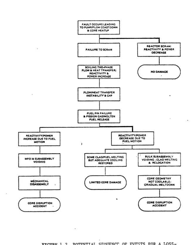
Figures 1.1 and 1.2 are taken from the Department of Energy's report on sodium boiling (1), and illustrate the complex sequences of events which have been developed for sodium boiling accidents. The heavy lines indicate the most likely sequences.

1.2 Scope of the Work

This project was conceived as an attempt both to model and simulate sodium boiling behavior, as part of the total D.O.E. effort in this area. Results from the Thermal-Hydraulic Out-of-Reactor Safety Facility (THORS) tests at

Oak Ridge National Laboratory have indicated that stable sodium boiling may be expected under low-power, low flow

conditions, such as might occur during a LOPI (2); current models do not accurately predict this type of behavior. In addition, significant flow oscillations occurred during some of these experiments. Upon analysis of the THORS results, it appeared that these oscillations might aid in postponing

FIGURB 1.1 POTENTIAL SEQUENCE OF EVENTS FOR A LOSS-OF-PIPING-INTEGRITY ACCIDENT

FIGURE 1.2 POTENTIAL SEQUENCE OF EVENTS FOR A LOSS-OF-FLOW ACCIDENT

the dryout of the core.

Since sodium experimentation is both costly and rather hazardous, due to sodium's tendency to ignite spon-taneously in oxygen, a simpler approach was developed, using water as a simulant. The objectives of this project were:

1. Development of a simple, one-dimensional model for

flow oscillations under low-power, low-flow con-ditions. This model should be easily understood and incorporate the necessary physical basis for the flow behavior to be modelled.

2. Performance of a series of experiments - with water-to ascertain whether the model would predict ob-served behavior, as well as to demonstrate the suitability of water as a simulant for liquid sodium.

3. Establishment of a set of criteria through which water and sodium experiments might be compared. 4. Comparison of data from the experiment to sodium

data using the criteria developed under 3.

The fourth objective was to be met through com-parison of the results obtained from the water experiments to those from the Sodium Boiling Test Facility (SBTF) at ORNL.

the model, choice of the simulant, criteria for the compari-son of water and sodium experimental results, the design of the M.I.T. Water Test Loop, and the results and analysis of experiments performed on the WTL. A brief description of the SBTF will also be included. Finally, the conclusions from this work are presented, along with recommendations for future work in this area.

CHAPTER 2

THE ANALYTICAL MODEL 2.1 Overall Concept

The modelling of two-phase flow is an extremely complex task, due to the interactions of the phases with each other, as well as with their surroundings. Because of this fact, the model developed for this work was derived so as to keep the vapor phase essentially separated from the liquid. In addition, the flow oscillations to be modelled involve the expansion and contraction of a vapor space surrounded by two nearly incompressible liquid columns. The growth and collapse of such a bubble can be the result of either of two effects: a hydrodynamic effect, whereby the vapor space grows or collapses due to the differential pressure between the bubble and the liquid, or a thermal effect, through which the amount of vapor increases or de-creases through the evaporation or condensation of the vapor. This second mechanism requires the transfer of heat, either latent or sensible, whereas the first does not. The two effects do not occur independently, however; the collapse of a steam bubble due to hydrodynamic effects would tend

to increase the bubble pressure. This would then raise the saturation temperature of the bubble and cause condensation

to occur, possibly causing further collapse and starting the cycle again.

Due to the two possible methods of bubble growth and collapse, the model has been developed so as to incor-porate both of these factors. This approach was proposed by Ford (3) in his freon experiments and modelling. While Ford's original reasoning was followed, the details of the models differ, as well as the methods of solution.

In developing this model, the objective was to produce what would eventually be a module in a large system-scale code. There was no attempt made, therefore, to model the single phase flow configuration prior to the inception of boiling and flow oscillations, nor were there any means provided to carry the calculation past the point at which

the limitations of model occur. The model limitations are discussed in Section 2.5, and recommendations for further calculational tools are presented in Chapter 6.

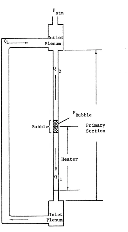
2.2 The Hydrodynamic Model

The system under consideration for the develop-ment of this model is illustrated in Fig. 2.1. The vapor

space is assumed to be at constant pressure throughout, and the top of the upper plenum is assumed to be at atmospheric pressure. The liquid is considered to be incompressible, and acts essentially as a piston. The vapor space is not

Patm t e Plenum PBubble Primary Section

A-I

assumed to be incompressible; in fact, its compressibility is one of the driving forces in the oscillations.

The system is assumed to be in a fixed configur-ation, with the vapor slug totally separated from the liquid. This "fixed-regime" type of model allows a simple mathemati-cal description of the system.

The momentum equation for one-dimensional, incom-pressible, single phase flow in a pipe is

dv 1 dp 1 dT

::- = f (2 1)

dt p dx p y x

Integrating over the volume: dv

p _z AL _dt = AAP - A T - F (2.2)

shear x A

K

This equation can be rearranged to show the contribution

of each term:

APtot = AP tt acc+ acc APfric fric + APgrav grav (2 3) The first term represents the acceleration of the fluid; the second is the pressure drop due to friction, and the third term represents the pressure drop due to body forces, in this case, gravity.

dv

If the area is assumed constant, the term pALdv

ddQ can be expressed as pL -, where Q is the volumetric flow rate, vA.

Dividing Eq. (2.3) by the area, and combing the gravitational and total pressure drops

P9L dQ

AP' =A dt+ Ashear ( 2.4)

A

where AP' = AP - AP .

tot grav

The frictional term is now expressed, as is custom-arily done, using a friction factor, f:

2

L Pv t _ A

AP 4f AT shear (2.5)

fric D 2 KA

Casting the equation in terms of the volumetric flow rate,

Q,

A

Equation (2.4) now becomes

AP'

=

(p-L

dQ +

A

A dt D A2

The term pL is the inertance of the fluid column A

indicated by I. The term 2fLpQ/DA2 is the effective resist-ance due to friction on the fluid, and is indicated by R. Thus

AP' = dQ + RQ (2.8)

This form of the equation is commonly used in system dynamics, and allows the creation of an electrical analog, with pres-sure drop paralleling voltage and volumetric flow rate analog-ous to current. The coefficients I and R would correspond to circuit inductances and resistances, respectively.

In Eq. (2.8), the pressure drop AP' represents the non-gravitational pressure difference between the vapor space and the constant upper plenum pressure, and is common to the two liquid legs.

The equation for the vapor space is also derived from system dynamics. For a compressible volume, the con-servation of mass equation states

dm d (PV ) p Q (2.9) dt dt gg gg thus V d dV Q = - d + - (2.10) g p dt dt

If the motion of the boundaries of the compressible volume is examined, it is seen that the motion of the liquid legs, hereafter referred to as Q1 and Q2, sum to the volume change, dV --. Therefore, dt V dp Q = ---9 (2.11) com p dt 3 g

Using Eq. 2.8, the equations for the two liquid legs shown in Fig. 2.1 can be expressed as

dQ1 AP' = I _{1 dt} d + R _{1 1}Q1 dQ2 AP' = I2 !- _{2 dt} + R_{22 2}Q2 since Q1 + _Q2 dv dt (2.12) (2.13) (2.14)

As stated above, Eqs. (2.14) and (2.11) can be combined to define a source volumetric flow rate, Qs, such that

Q0 + Q2 + Q3 = Q (2.15)

The four equations, 2.8 (one for each liquid leg), 2.11, and 2.12 comprise the hydrodynamic model.

2.3 The

directly system.

Thermal Model

The thermal model for bubble growth is derived from the first law of thermodynamics for a closed That law states:

6q - 6W = 6U

The definition of enthalpy

H = U + PV

(2.16)

is substituted into Eq. (2.16). Realizing that the term 6W represents pressure-volume work done by the system, so that

6W = P6V (2.18)

and making this substitution, as well, Eq. (2.16) becomes

6q - P6V = 6H - P6V - V6P (2.19)

or

6q + V6P = 6H (2.20)

Equation (2.20) is now divided by 6t, and the

limit is taken as 6t approaches zero. This gives the diff-erential form of the equation

+ dP

dt dt

dH

dt (2.21)

The enthalpy term for a two-phase system can be separated into its components. Thus

H = m h + m h (2.22)

dH

_-:

g dt dt g dt and

The system of bubble and surrounding liquid is chosen to be large enough so that the mass fluxes across the system bound-aries are zero. This choice of a closed system sets a model

limitation. This assumption is valid only when the vapor through-flow in the bubble is very small, a condition which exists for small bubble lengths only, as in the early stages of a transient. From the definition of a closed system, therefore dm_{dm =} 0 (2.24) dt and dm dm - 9= - (2.25) dt dt

Substituting into Eq. (2.20):

IT

dm

dh

dh

d (h - h d- m +m (2.26)

S= g L dt m dt gdt

The last two terms represent the change in sens-ible heat of the system. For small changes in temperature and pressure, these contributions are negligible when com-pared to the latent heat of vaporization, (h - h£) or hfg. Thus,

dm

dH h dm (2.27)

Substituting back into Eq. (2.18) yields dm dq + V dP =h dm _{(2 .28)} dt dt fg dt Since mg = p V g g g dm V dp dV = g - + P (2.29) dt dt dt and dv V dp + V dP + = ( V gP/@h (2.30) dt p dt dt g h fg g gf

It should be noted that the left hand side of Eq. (2.30) corresponds exactly to the source flow Qs [Eq.

(2.15)] derived in Section 2.2. Equation (2.30) comprises

the thermal model for the system.

2.4 Solution of the Equations

The thermal and hydrodynamic equations for the system are solved simultaneously and iteratively to find the net source flow and the bubble behavior. The solution is accomplished by means of a digital computer, using a program developed as part of this project.

dQl AP' = I1 + R' Q (2.31) 1 dt 1 1 dQ2 2 AP' = 12 _{2 dt 2} + R'2_{2 2}Q 2 (2.32) V dp Q = d (2.11) 3 p dt g s (net + _{V )/ph = Q1} + Q _{3 (2.30)}

In rewriting these equations, the subscripts 1 and 2 refer to the two legs noted on Fig. 2.1; subscript 3 refers to the bubble itself. The total net heat flow to the bubble is symbolized by net. Since the resistance term, R, depends on Q [Eq. (2.7], a new coefficient, R', has been introduced in Eqs. (2.31) and (2.32), such that

' = 2f -- 1 (2.33)

D 2

A

There is still a dependence of R' on Q, since the friction factor, f, is a function of the Reynolds number and

Re = pQD (2.34)

Ap

However, since this dependence is normally to a small frac-tion power in turbulent flow, the form in Eq. (2.33) has

been retained.

The number of bypass legs that are part of Leg 1 in Fig. 2.1 is immaterial since, by the analogy of parallel resistances and inductances, these can be combined into an effective single bypass leg. Additional resistances, such as elbows, tees, and other flow obstructions can be accomo-dated using an equivalent resistance concept, as well.

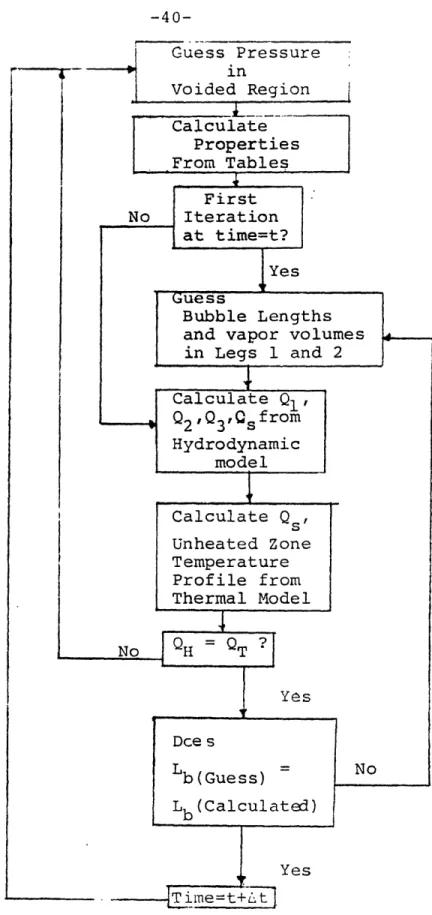
The solution scheme employed in the computer pro-gram sets the equations up in finite-difference form and solves them iteratively. Equations (2.31) and (2.32) are approximated by first order, explicit finite difference equations, while Eqs. (2.11) and (2.30) are solved by im-plicit first order difference equations. Details of the solution scheme may be found in Appendix A. The iterative technique itself consists of the following steps:

1. The pressure in the bubble is guessed, as well as

the bubble lengths and vapor volumes, above and within the heater. The split must be made due to the fact that in the heated zone, evaporation occurs, while in the unheated section above the heater, evaporation occurs. Thus, in order to de-rive the net heat input to the vapor space, which is the difference between evaporation and conden-sation, the bubble must be split into two parts. The common vapor space pressure ties the two parts

together.

2. The pressure guess allows the determination of the properties in the bubble, since the assumption is made that all vapor (as well as the liquid film on

the walls of the heater) is at saturation. The liquid density is assumed to be constant, and

equal to that at saturation. This allows direct solution of Eqs. (2.11) and (2.27), since net heat input is a function of temperature and power to the heater. Other iterative loops determine the amount of power that goes into heating up or cooling the

heater wall as pressure changes and the temperature profile of the liquid in the unheated section, as heat is introduced into this liquid by condensation. 3. Equations (2.31) and (2.32) are solved as described

above.

4. The source flow (Q₁+Q +Q ) calculated from the thermal model is compareA to that calculated from

the hydrodynamic model. If these two flows are different by more than a specified convergence

error limit, a new pressure is guessed and the cal-culation starts again from step 1.

5. If the two source flows are within the specified error, new bubble lengths and vapor volumes are calculated and compared to those that were guessed

in step 1. If these are within a specified toler-ance, time is incremented and the transient calcu-lation proceeds. If they are not within the error limit, a new guess is made of bubble lengths and volumes, and the calculation returns to step 1 for another iteration.

A flow chart is shown in Fig. 2.2 illustrating this technique.

As noted in step 2 above, a temperature-time his-ory of the upper unheated zone is calculated. This is done in order to allow calculation of the condensation of vapor which occurs in that part of the test section. The model

used for this calculation is a nodal-averaged temperature scheme, whereby the upper section is split into a number of nodes, each with a single temperature, and new

temper-in

Voided Region

atures are calculated based on the flow of liquid into and out of each node, as well as any condensation which might occur. The changing temperature in the unheated section determines the thermal contribution to bubble growth and collapse, and changes in the amplitude and period of oscil-lations may be related to this factor. Further discussion of this fact is found in Chapter 5. Details of the temper-ature calculational scheme can be found in Appendix A.

The method of solution outlined in this section has proven to yield satisfactory and physically realistic results. These results, along with comparison to experi-mental results can also be found in Chapter 5.

2.5 Limitations of the Model

A "fixed-regime" model is valid only insofar as the regime that is fixed actually exists physically. Once conditions proceed to a point where the assumptions incorpo-rated into the model are no longer justifiable, the model is no longer useful in describing the system.

In the case of the model presented here, the model is valid for small bubble lengths and vapor volumes.

Due to the assumptions made in both the hydrodynamic and thermal portions of the model, any deviation from a slug-flow regime would cause the model to fail. In addition, liquid and vapor through-flows are neglected in the

formu-lation of the thermal model. When the bubble becomes large enough to encourage substantial natural circulation flow, this assumption becomes invalid. For these reasons, once net evaporation exceeds net condensation, causing the bubble

to grow without collapse, the transient calculation is stopped, and the assumption is made that another calculational tool

CHAPTER 3

CRITERIA FOR THE COMPARISON OF BOILING LIQUID SODIUM TO WATER

3.1 Background

The application of data from water experimentation to the question of what occurs during the boiling of liquid sodium requires that a group of criteria be developed with which to compare water data to sodium data. Several such

criteria will be proposed in this chapter.

Clearly, the physical characteristics and proper-ties of the two fluids are quite different, especially those properties dealing with heat transport. Therefore, heat

conduction is not included in the comparison criteria. It is assumed that different temperature profiles may exist under the same flow conditions in water and sodium, and

differences arising from this fact must be considered.

However, from inspection of the equations of the model pre-sented in Chapter 2, it can be seen that the properties

that affect the equations are largely hydrodynamic in nature,

and there is substantially less disparity between water and

liquid sodium in this area. Table 3.1 lists both thermal and hydrodynamic properties of each fluid for comparison.

Table 3.1

Comparison of Water and Sodium Properties

Fluid Property Tsat P pz/P hfg Cp Water at 14.7 psia 2120F 59.8 lbm/ft' 0.0373 lbm/ft 1603 970.3 BTU/lbm 1.0 BTU/lbmoF 0.687 lbm/hr-ft 0.004 lbf/ft 0.394 BTU/hr-ftoF Sodium at 25 psia (Reactor Conditions) 16700_F 46.4 lbm/ft3 3 0.025 lbm/ft 1650 1650 BTU/lbm 0.31 BTU/lbmoF 0.363 lbm/hr-ft %0.012 lb /ft 31.5 BTU/hr-ftoF

The criteria developed in this chapter, then, are mainly hydrodynamic in nature, and may be used under these

special circumstances to compare boiling water to boiling liquid sodium.

3.2 Momentum Equations

The approach that is taken throughout this chapter involves the non-dimensionalization of the basic equations.

The momentum equation, as presented in Chapter 2 for Unidimensional, single phase flow in a oipe is:

2

dv _ 1 d d2 v - f (2.1)

dt p dx P 2 x

The body force--fx- is, in this case, due to gravity; thus

2

dv 1 dp d v_{2 g (3.1)}

dt p dx P dy2

Non-dimensionalization is accomplished by choos-ing new variables that are dimensionless. For the momentum equation, these variables are:

v = o/poop

v* = v/v 0 (3.2)

y* = y/D

p*= p/p₂,

P* = P/P

x* = x/D

P1* = P/Pz

The quantity P is a reference pressure, and D is the diameter, and serves as a reference length scale.

Substituting these quantities into Eq. (3.1) yields

2

Vo dv* o 1 dP* P Vo * d2v *

D dt* pPD p* dx* p D2 p* dy*2 g

(3.3) Simplifying, and applying the definition of v [Eq. (3.2)] to the first term on the right hand side:

dv* _ 1 dp* P 9£ _* d2v* Dg (3.4)

-1- (3.4)

dt* p* dx* pz voD p* dy* d*2 v 2

The coefficient of the second term on the right hand side of the equation is the inverse of the Reynolds number. This is the first of the comparison criteria. The Froude number also appears, as the last term in Eq. (3.4). Although this sets another criterion, it reduces essentially

to a density ratio for systems of similar geometry and pressure. Applying the definition of v₀ to the expression

Dg yields the result 2 v 0 Dg

_{E = 94}

_g(3.5)

Since the liquid densities of sodium and water are similar, this criterion is satisfied. The choice of another geometry, however, would necessitate consideration of this parameter.

The appearance of the Reynolds number is not al-together unexpected. As stated above, the driving factors in the oscillatory flow behavior tend to be chiefly hydro-dynamic in nature; thus, the prime basis for hydrohydro-dynamic scaling should appear.

3.3 The Compressibility Equation

The term expressing the compressibility effects is

V dp

Q = -2 ' (2.11)

g p dt

The volumetric flow rate is defined in Chapter 2 as Q = Av g Thus V dp Av = -1 - (3.6) p dt

or

V dp

A x -2 " 9

dt pg dt

Once again, dimensionless variables are chosen:

x* = x/D A* = A/D 2 V * g = V /D 3 g t* = t/T p*= Pg/p

Equation (3.7) now becomes

3A• D A* T D3V *P dx* D a k dp* dt* pT dt* Simplifying: A* dx* = P d p * dtA* g dt* g (3.7) (3.8) (3.9) (3.10)

The second dimensionless group, then is the liquid-to-vapor density ratio, PZ/p . This term behaves as a kind

of variable spring constant, since it changes with pressure, and along with the length of the bubble and heat transfer, helps to determine the oscillatory behavior of the system. From the table of properties, it is clear that the density ratios for sodium and water at pressures near atmospheric are similar.

3.4 The Energy Equation

The energy equation, as derived in Chapter 2, is

dV V dp VdP

9 + 9 __1 = (4 + 9 )ph (2.27)

dt p _g dt at g fg27)

The left hand side of the equation is equivalent to a volumetric vapor generation rate, Qs. The term VdP/dt is very small compared with the net heat flow, 4, and is neglected.

Thus

Qs net / ghfg (3.11)

The source flow, Qs , can be expressed, as in the previous section, in terms of an equivalent velocity and area:

Avs = net/ ghfg (3.12) The velocity, v , is now non-dimensionalized:

s v *= V s/v (3.13) Then Avo s* = net/pghfg (3.14) and finally vs = net/pgVo A hfg (3.15)

The net heat input includes both power input to the lower part of the bubble, as well as condensation which occurs when vapor enters the unheated section above the heat source. The vapor generation occurs via evaporation at the liquid-vapor interface, at saturation, and the

con-densation is due to the interaction of saturated vapor with subcooled liquid. If this heat input is expressed in terms of an equivalent heat transfer coefficient and temperature

difference, Eq. (3.15) becomes h (T-T ) v* = eq sat (3.16) s Pgv hfg where (3.17) 4_net = heq A (T-Tsat )

The quantity on the right hand side of Eq. (3.16) is the Jakob number, Ja, multiplied by the Stanton number, St, since C p Cpt (_sat) Ja = (3.18) pghfg_{pg hfg} and h St = h (3.19)

More importantly, this combination serves as a kind of power-to-flow ratio, normalized by the latent heat of vaporization. It is this term which should be used as a comparison criterion. The factor of differing saturation temperatures is also taken into account. One factor which appears indirectly in Eq. (3.16) is the condensation in the unheated zone, since it is combined with the heat input term. The condensation potential in the unheated section appears to be the primary driving force in the flow oscill-ations under study, a fact that will be discussed more

fully in Chapter 5. The heat input to the system is effec-tively a constant over the duration of the experiments, and it is this condensation term which provides the variation in

4net

3.5 Comparison of Sodium Data to Water Data

The Sodium Boiling Test Facility (SBTF) at Oak Ridge National Laboratory is almost an exact analog of the original MIT Water Test Loop, as described in Chapter 4. The SBTF also has a pump to provide for forced-flow experi-mentation; however, it does not include a bypass loop at

this time.

The SBTF is a sodium loop, heated indirectly over its three-foot heated length by a quadelliptical radiant furnace. At the inception of this program, it was expected that some data would be available from SBTF in order to provide a direct comparison to water data. While several of the natural circulation tests performed on the original WTL have been reproduced, budgetary and experimental prob-lems have forced a delay in the performance of forced-flow

and flow oscillation testing. It is anticipated that these

types of experiments will be performed in the near future, providing a direct test of the comparison criteria herein proposed.

CHAPTER 4

EXPERIMENTAL APPARATUS AND PROCEDURES 4.1 Background and Experimental Apparatus

The expense and hazard involved in the use of liquid metals as an experimental medium led to the concept of the first M.I.T. Water Test Loop, constructed by Dr. W. D. Hinkle in 1976. The WTL was intended to be a simple,

easy-to-operate alternative to complex sodium boiling facili-ties such as THORS. The first experiments performed and re-ported by Hinkle (4), involved natural circulation tests only, to determine critical heat fluxes under low-power

conditions. These results, along with comparison criteria developed by Hinkle, were compared to sodium data obtained under similar conditions from the SBTL loop at Oak Ridge (5). Water was chosen as the simulant in the initial series of tests because of the similar liquid-to-vapor density ratios

for the two liquids. Other similarity criteria were not considered.

Flow oscillations such as those observed in the THORS tests could not be modelled using Hinkle's approach, and so a more involved and sophisticated test program was developed. The performance of these experiments required that the Water Test Loop be modified somewhat from its

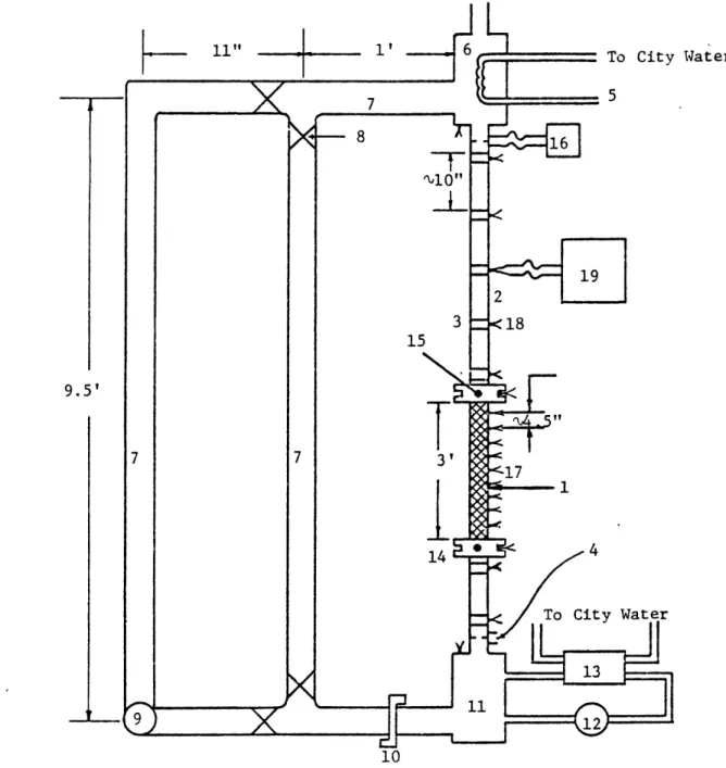
original design. Figure 4.1 shows the loop in its current configuration; Table 4.1 lists the dimensions and properties of the loop. The modifications consisted of the addition of a pump and a bypass leg, which would allow operation in

either forced or natural circulation. Four ball valves were installed at the bypass to provide the means to change flow configurations. In addition, an orifice flange was added upstream of the inlet plenum to provide the capacity to vary the inlet flow resistance. Whereas the entire

"primary" section - that part between the two plena

con-sisting of the heater and unheated inlet and outlet sections-had been steel, the new loop was built with Pyrex glass

tubing making up as much of the unheated sections as practi-cal. This allowed visual observation of bubble growth and collapse patterns during a transient.

The instrumentation was also altered considerably for the new tests. Thermocouples had previously been fast-ened to the outside of the entire metal primary section, and strain-gauge type pressure transducers were installed in the inlet plenum, heater inlet and heater outlet. There was no flow measuring instrument included. Data acquisition was by means of a chart recorder. The modified version of the loop retained the thermocouples on the outside of the heater rod; however, the Pyrex sections were split into

11" -1' _{To City Water} -]-J 7 - 8 _-16 19 2 3 <18 15 9.5' 7 7 3' 144 To City I

jL

'

13

Note: Numbers refer to Table 4.1 on following page

Table 4.1. List of Loop Components

Component Number Function

Heater Tube - 0.25" OD

Pyrex Tubing - 6mm OD

Swagelok Tee for Thermocouple Insertion

Orifice for AP Transducer

Cooling/Heating Coil for Plenum

Upper Plenum - 8"I.D. x 8" ht.

Stainless Steel Bypass Pipe -1" I.D.

Ball Valve for Flow Control Pump

Orifice Flange

Lower Plenum 8" I.D. x 8" ht.

Heat Exchange Loop Pump Heat Exchanger

Connection to 7kw DC Generator Insulator and Tyco Pressure

Transducer

Validyne AP Cell across Orifice Thermocouple on Outside of

Heater Tube

Thermocouple Inserted into Swagelok Tee

smaller zones, with each end inserted into a Swagelok tee. The third port of the tee was used for insertion of a thermo-couple directly into the fluid stream. The thermothermo-couples were sealed into the ports using RTV Silicone Rubber Sealant. All thermocouples were copper-constantan.

Pressure transducers of the same type that Hinkle used were retained for the heater inlet and outlet. The inlet plenum transducer was not used. These gauges were Tyco type AB, with a range of 0-6 psig. When excited by a 6-volt dry cell battery, the response was linear, at a rate of 20 mv/psi.

For the new set of experiments, it was desired to have measurement of inlet and outlet flow rates. To accomp-lish this, flow orifices were installed just downstream of the inlet plenum and upstream of the outlet plenum. The orifices were about 80% of the test section diameter. They were made this way so as to cause as little interference with the flow as possible, while still generating enough of a pressure drop to measure flow rate. Pressure drop measurements were made using Validyne DPl5 differential pressure transducers. These instruments can be adjusted as to the range of their output, from about ± 0-1 to ± 0-10 volts full scale. The transducers themselves are vari-able reluctance devices with interchangevari-able diaphragms,

permitting operation from ± 0-0.1 psid upward. In order to provide response as accurate as possible and to avoid pinning

the data acquisition system at its maximum output, a range of ± 0-1 volt was chosen, with the lower transducer set for

+ 0-1.0 psid, and the upper transducer for ± 0-0.5 psid.

The Validyne transducers were supplied with their own carrier demodulators, which served as both a power source and voltage output device. Calibration of these transducers was done

in place, using both upflow and downflow.

The loop was run in visual observation tests immediately after construction. On the basis of these ob-servations and sodium test results, the decision was made to purchase a fast-scan data acquisition system, in order to collect data at a rapid enough rate to be able to trace the oscillatory motion. The system chosen was a Perkin-Elmer Low-Level Real Time Analog System (RTAS). The RTAS has the capability of scanning individual data points at rates up to 8000 points per second. The low level system permits inputs of ± 0-1.0 volts. To collect and store the data, a Perkin-Elmer Model 1610 minicomputer was acquired. This machine is a 16-bit computer with 64000 bytes of

memory, with dual floppy disk drives to provide input-out-put capability. A Perkin-Elmer 550 CRT terminal was used as the system console, and a Perkin-Elmer 650 Thermal Printer

was connected to the rear of the CRT to provide hard copy output, if desired. Operating system software, including FORTRAN support,was supplied by Perkin-Elmer. Using the

1610 computer and driver programs developed by Perkin-Elmer for the RTAS, data acquisition was done at the rate of 600 points per second. The RTAS input supports twenty-four

individual instruments, and scans were performed twenty-five times per second. The instrumentation consisted of: The

two Validyne differential pressure transducers, the two Tyco gauge pressure transducers, and nineteen thermocouples, one each in the inlet and outlet plena, eight tied onto the

out-side of the heater at approximately 4.5 inch intervals, and nine in the unheated zones. The twenty-fourth point was

connected to an RTD temperature reference on the RTAS term-ination panel to provide an equivalent ice-point for the thermocouples. The computer, through its line-frequency clock, is able to generate interupts at up to 120 times per second. Each interupt allows the RTAS to scan all 24 points at the maximum scan rate. The interupt interval

chosen for these experiments was 40 milliseconds. More detail on the data acquisition system can be found in Appendix B.

Power was supplied to the test section by a 7 kilowatt DC generator. The test section was directly

heated (resistance heating) by the generator. Power was measured using a Hewlett Packard Model 3465 B Digital Multi-meter. The voltage drop across the test section heater tube was measured, and multiplied by the generator current output.

Generator current was ascertained by means of a calibrated shunt providing 50 4v output at 1000 amperes.

The remainder of the test section, aside from the bypass legs, consisted of a heat transfer loop to cool the

plena. The lower plenum was cooled by direct fluid exchange,

whereby fluid was removed, pumped through a small heat ex-changer, and returned to the plenum. The upper plenum, which was open to the atmosphere to provide a constant reference

pressure, was cooled by a copper coil loop inside the plenum. Water was run from the city water pipes through this copper coil, and the temperature of this water could be varied, so as to hold the plenum at the desired temperature.

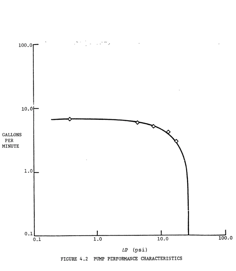
Both the main test section pump and the heat ex-changer loop pump were Jabsco "Sturdi-Puppy" self-priming

vane pumps, rated at 5 gpm at 8.5 psi. Figure 4.2

repre-sents the pump curve.

The bypass legs were stainless steel piping. The large size of these pipes in relation to the primary tubing was to negate any significant bypass effect on flow dynamics.

100.0 10.0 GALLONS PER MINUTE 1.0 0.1 0.1 1.0 AP (psi)

FIGURE 4.2 PUMP PERFORMANCE CHARACTERISTICS

4.2 Experimental Set-up and Procedure 4.2.1 Pretest Set-up and Calibration

Prior to each set of experiments, several steps were followed to insure readings from instruments were as accurate as possible. With the loop filled, the battery for the Tyco pressure transducers was checked to make cer-tain it still was charged at 6 volts. The transducers themselves were then checked for offset from zero. This was accomplished by checking the output from each trans-ducer with a digital multimeter to ascertain the output, and then subtracting from that reading 20 my for each psi of water head above the transducer.

The second step involved the calibration-in-place of the Validyne differential pressure transducers. Each transducer was calibrated in both upflow and downflow. Calibration in upflow was accomplished via a two step method. The loop was run at the beginning of the experi-mental program with the bypass line opened and the power at a low level. Using the thermocouples directly upstream and downstream of the heater, a heat balance was performed. Knowing the amount of power input and the temperature size of the water across the heater, it was then possible to determine the flow rate. This single point was used to calibrate the transducers in upflow, with the assumption

of linear transducer response. For downflow calibration, the primary side of the loop was isolated to prevent re-circulation effect on the transducer. Water was then with-drawn from the lower plenum through the hole where the plenum pressure transducer had been mounted in Hinkle's experiment. Initially, since the water could be withdrawn at variable rates, several different measurements were made. The flow was collected for a timed interval, then measured to find the flow rate. The rate of withdrawal was sufficiently

small, so that the driving pressure on the primary side did not change appreciably. This insured constant flow over

time. The calibration with several points verified the linearity assumption made in upflow, and in later calibra-tions, only one point was taken for downflow calibrations. The transducers themselves were first bled, and then zeroed using the carrier demodulator adjusting dial. Output was again read using a digital multimeter.

Before beginning experimentation, the loop was operated for several minutes to remove all trapped air bubbles from the system.

The final step before beginning the experiment was to load the data acquisition system controller programs

into memory. Once this was accomplished, the data collection procedure could be started by simply pressing on key