Parameters estimation from the gravity anomaly caused by the two-dimensional horizontal thin sheet applying the global particle swarm algorithm

(1)

HAL Id: hal-02867638

https://hal.univ-lorraine.fr/hal-02867638

Submitted on 6 Oct 2020

HAL is a multi-disciplinary open access

archive for the deposit and dissemination of

sci-entific research documents, whether they are

pub-lished or not. The documents may come from

teaching and research institutions in France or

abroad, or from public or private research centers.

L’archive ouverte pluridisciplinaire HAL, est

destinée au dépôt et à la diffusion de documents

scientifiques de niveau recherche, publiés ou non,

émanant des établissements d’enseignement et de

recherche français ou étrangers, des laboratoires

publics ou privés.

Parameters estimation from the gravity anomaly caused

by the two-dimensional horizontal thin sheet applying

the global particle swarm algorithm

Khalid Essa, Yves Géraud

To cite this version:

Khalid Essa, Yves Géraud. Parameters estimation from the gravity anomaly caused by the

two-dimensional horizontal thin sheet applying the global particle swarm algorithm. Journal of Petroleum

Science and Engineering, Elsevier, 2020, 193, pp.107421.

�10.1016/j.petrol.2020.107421�.

�hal-02867638�

(2)

Parameters estimation from the gravity anomaly caused by the two-dimensional horizontal

thin sheet applying the global particle swarm algorithm

Khalid S. Essa

a,*

_{, Yves Geraud}

b

a _{Department of Geophysics, Faculty of Science, Cairo University, Giza, P.O. 12613, Egypt}b Université de Lorraine, CNRS, GeoRessources, F-54000 Nancy, France

A R T I C L E I N F O Keywords: Gravity anomaly Depth Width Two-dimensional sheet Oil exploration A B S T R A C T

A global particle swarm algorithm utilized to assess the inverted two-dimensional horizontal thin sheet parameters from the gravity anomaly profile based on applying the second moving average method. The using of the second moving average method has more advantageous than using the Bouguer gravity anomaly because this method has a capability in eliminating the regional field up to third-order impeded in the Bouguer anomaly. This algorithm is applied to interpret the gravity anomaly profile, i.e., estimating the depth, the width, the thickness, the density contrast and the origin location of the buried structure. The efficacy and stability of this method are investigated and exposed for utilizing free-noise and noisy synthetic examples. Real gravity data associated with oil and gas and mineral exploration from three different locations around the world is interpreted. The evaluated time to discovering this appropriate clarification is very short and the estimated parameters contrast the view that the proposed method is applicable for real exploration. It can extract the inverse parameters which have a geologic and economic significance.

1. Introduction

Gravity anomaly interpretation is beneficial in discover areas that have anomalous under the surface. Besides, the numerous application of gravity method in oil, gas, ores, and minerals exploration, engineering applications, geothermal ancient civilization investigations (Essa, 2013; Abdelfettah et al., 2014; Mehanee, 2014; Aydemir et al., 2015; Mehanee and Essa, 2015; Deng et al., 2016; Biswas et al., 2017; Al-Farhan et al., 2019). Gravity data interpretation is ill-posed and non-unique which is evident through various geometric-shapes of subsurface structures that can produce similar gravity anomaly at the surface of the earth. So, we minimize this non-uniqueness and ill-posedness by finding the desired geometry for subsurface targets with an identified density followed by the inversion process (Eshaghzadeh et al., 2019).

The target of this study is to discover and figure out the two- dimensional horizontal thin sheet, which resembles magma intrusion in sedimentary covers (Kearey et al., 2002). The evaluation of the depth, thickness, and width of the buried bodies is very important in assessing the importance of buried economic targets.

Many scientists showed and deliberated different methods for inferring gravity data due to this source (Skeels, 1963; Pick et al., 1973). Nevertheless, the shortcomings of these approaches that rely on specific points and curves are focus on human inaccuracies in figuring the parameters of the buried structures (Essa, 2014). So, there is still a necessity for an inversion elucidation method that is accurate, vigorous, fast and gives approximately real geometry parameters of the forms in field cases. In addition, the accuracy of appraising the depth and the width relies on the accuracy of separating the residual field from the observed gravity data. Abdelrahman et al. (2016) established a least-squares algorithm to calculate simultaneously the depth and the width of a buried two-dimensional thin sheet from moving average residual gravity anomalies applying the window curves method. The main drawback of using the window curves method is entrapped in local minima. In other words, the intersection of the window curves intersect in different solution and sometimes not converge.

Thus, a gravity anomaly profile generated by a finite two- dimensional thin sheet was studied to infer the buried thin sheet parameters (the depth, width,

thickness, the density, and the origin location) including a different level of noise (0%, 5%, 10%, 15%, and 20%)

and multi-sources to measure the robustness and the consistency of the suggested method. Besides, this method is confirmed by three field examples from Canada, Cameroon, and Iraq.

2. The method

The general observed gravity anomaly is represented by the following form:

Total xj ¼ g xj; h;w þ Regional xj ; j ¼ 0; 1; 2; 3;…; N (1) where TotalðxjÞ represented

the collected gravity data, gðxj; h;wÞ represented the residual gravity

anomaly for the two-dimensional thin sheet, which is mentioned below, and

RegionalðxjÞ is the regional background field (Pawlowski, 1994; Obasi et al.,

2016; Essa and Munschy, 2019). 2.1. The two-dimensional thin sheet model

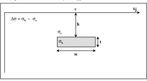
The profile of gravity anomaly (mGal) generated by the finite two- dimensional horizontal thin sheet (Pick et al., 1973: Abdelrahman et al., 2016) along the profile is:

(2) where h is the depth to the center (m), w is the width of the sheet (m), xj is

the survey positions (m), c is location of the central point of the anomaly (m), Δσ _{is the density contrast among the target and the surrounds g=cc , G is the}

universal gravitational constant parameter that equals 6.67 10 11 _m3_{kg s}₂_,

and t is the thickness (m). Fig. 1 shows a sketch for the two-dimensional

and multi-sources to measure the robustness and the consistency of the suggested method. esides, this method is con rmed by three eld e -amples from anada, ameroon, and ra .

2. t od

he general observed gravity anomaly is represented by the following form

Total!xj"¼ g!xj;h; w"þ Regional!xj"; j ¼ 0; 1; 2; 3; …; N

where otalð Þ represented the collected gravity data, ð ; h; Þ repre-sented the residual gravity anomaly for the two-dimensional thin sheet, which is mentioned below, and e ionalð Þ is the regional bac ground

eld Pawlows i, basi et al., Essa and unschy, .

he t o imensional thin sheet mo el

he pro le of gravity anomaly mGal generated by the nite two- dimensional horizontal thin sheet Pic et al., Abdelrahman

et al., along the pro le is

g!xj;h;w"¼2GΔσt # tan%1$w%2!xj% c " 2h % þtan%1$wþ2!xj% c " 2h %& ; j¼0; 1; 2; …; N

where h is the depth to the center m , w is the width of the sheet m , is the survey positions m , c is location of the central point of the anomaly m , Δσ is the density contrast among the target and the sur-rounds '=_cc

(

, G is the universal gravitational constant parameter that e uals . & % )_{m *}

& s +

, and t is the thic ness m . ig.

shows a s etch for the two-dimensional horizontal thin sheet and all parameters are demonstrated.

he secon mo in a era e metho

he second moving average method is considered as one of the pioneer methods in separating the regional bac ground eld, which is represented by a mathematical polynomial up to a third-order Grif n,

Essa and unschy, . he second moving average regional

anomaly along the pro le is

R2!xj;z; s"¼6g!xj

"_{% 4g!x}

jþ s"% 4g!xj% s"þ g!xjþ 2s"þ g!xj% s"

4 ;

where s is the window lengths. urthermore, the interpretation involves only a relatively long pro le length, the problem of applying short pro le lengths may be overcome effectively and economically by increasing the measurements number through the constrained length of the pro le or digitizing the old gravity pro le using a suitable interval.

he lo al optimi ation particle s arm al orithm

he global optimization particle swarm is developed and introduced during the last years to solve many geophysical problems Sen and

Stoffa, Singh and iswas, Essa and Elhussein, Essa,

, Karc o!glu and G rer, . he particle swarm

progres-sion is stochastic and stirred by the communal repetitive in a ourney of birds for searching the foods where the birds are the models. he indi-vidually model has a position and velocity vectors where the position vectors signify the value of the parameters. he particle swarm is ad usted with random models and loo ing for sources by apprising generations. n every iteration step, each model modernizes its velocity and place utilizing the ne t formulas

Vkþ1 j ¼ c3Vkjþ c1rand ' Tbest% Pkþ1j ( þ c2rand h' Jbest% Pkþ1j (i ; Pkþ1 j ¼ Pkjþ Vkþ1j  :

where v is the th _{particle velocity at the} th _{iteration, P} _{is the present} th _{particle place at the} th _{iteration, rand is random numbers amongst}

½ ; (, c an c are cognitive and social parameters and e uivalent

Parsopoulos and rahatis, , c is the inertial coef cient that

controls the particle velocity and its value . he inspiration behind selecting and utilizing the particle swarm techni ue is to get a global solution of various geometrical bodies from the gravity data uic ly and point out the prominence of employing this techni ue between various conventional, non-conventional and optimization approaches. urther-more, uic merging to the optimum solution in real time in uence managing and well recital assessment. hen, synthetic and real e am-ples mentioned-below have been e amined to con rm the motivation of using the particle swarm method at any time in the future.

he t o imensional thin sheet parameters calculation

he started model is gradually re ned at every iterative-step to catch the optimum- t amid the measured and the calculated data. or each step, the body parameters h, w, t, Δσ, and c are improved to catch the paramount values by minimizing the subse uent ob ective function. he optimal-solution of the body parameters h, w, t, Δσ, and c attained

(3)

2

horizontal thin sheet and all parameters are demonstrated. 2.2. The second moving average method

The second moving average method is considered as one of the pioneer methods in separating the regional background field, which is represented by a mathematical polynomial up to a third-order (Griffin, 1949; Essa and Munschy, 2019). The second moving average regional anomaly along the profile is:

(3) where s is the window lengths. Furthermore, the interpretation involves only a relatively long profile length, the problem of applying short profile lengths may be overcome effectively and economically by increasing the measurements number through the constrained length of the profile or digitizing the old gravity profile using a suitable interval.

2.3. The global optimization particle swarm algorithm

The global optimization particle swarm is developed and introduced during the last years to solve many geophysical problems (Sen and Stoffa, 2013; Singh and Biswas, 2016; Essa and Elhussein, 2018; Essa, 2019, 2020; Karcıoglu and Gürer, 2019 ). The particle swarm progression is stochastic and stirred by the

communal repetitive in a journey of birds for searching the foods where the birds are the models. The individually model has a position and velocity vectors where the position vectors signify the value of the parameters. The particle swarm is adjusted with random models and looking for sources by apprising generations. In every iteration step, each model modernizes its velocity and place utilizing the next formulas:

(4)

(5) where vkj is the jth _{particle velocity at the k}th _{iteration, P}_kj_{is the present j}th

particle place at the kth _{iteration, rand is random numbers amongst ½0;1, c}₁

and c2 are cognitive and social parameters and equivalent 2 (Parsopoulos and

Vrahatis, 2002), c3 is the inertial coefficient that controls the particle velocity

and its value ˂ 1. The inspiration behind selecting and utilizing the particle swarm technique is to get a global solution of various geometrical bodies from the gravity data quickly and point out the prominence of employing this

technique between various conventional, non-conventional and optimization approaches. Furthermore, quick merging to the optimum solution in real time influence managing and well recital assessment. Then, synthetic and real examples mentioned-below have been examined to confirm the motivation of using the particle swarm method at any time in the future.

2.4. The two-dimensional thin sheet parameters calculation

The started model is gradually refined at every iterative-step to catch the optimum-fit amid the measured and the calculated data. For each step, the body parameters (h, w, t, Δσ, and c) are improved to catch the paramount values by minimizing the subsequent objective function. The optimal-solution of the body parameters (h, w, t, Δσ, and c) attained through applying the following objective function ðϕobjÞ

(6) where N is the observed points, Tj o is the observed gravity anomaly and Tj p is

the calculated gravity anomaly at the point xj

Finally, after estimated the body parameters (h, w, t, Δσ, and c) of the buried two-dimensional thin sheet, the complete error (ψ) between the observed and calculated fields are assessed by taking the square-root of Eq. (6).

3. Application to synthetic example

So, the examination of the accuracy and the benefits of the suggested approach were inspected through a synthetic finite two-dimensional thin sheet model of parameters: h ¼ 12 km, w ¼ 5 km, t ¼ 3 km, Δσ ¼ 1 g=cc, c ¼ 5 km, and profile length ¼ 100 km generated and containing a third-order regional field applying the following equation:

(7) Besides, this anomaly is subjected to various levels of noise 0%, 5%, 10%, 15%, and 20%. This gravity data inferred applying the global particle swarm algorithm using 100 models utilizing 100 particles. The optimum model parameters reached after 300 iterations and the range values of each parameter are demonstrated in Table 1. Table 1 validates the ranges of every parameter and the estimated results for each parameter at every window lengths (s-values). In addition, it shows the average value (φavg), uncertainty

and percentage of error (E-value) in every parameter and the ψ-value that and multi-sources to measure the robustness and the consistency of the

suggested method. esides, this method is con rmed by three eld e -amples from anada, ameroon, and ra .

2. t od

Total!xj"¼ g!xj;h; w"þ Regional!xj"; j ¼ 0; 1; 2; 3; …; N

where otalð Þ represented the collected gravity data, ð ; h; Þ repre-sented the residual gravity anomaly for the two-dimensional thin sheet, which is mentioned below, and e ionalð Þ is the regional bac ground

he pro le of gravity anomaly mGal generated by the nite two- dimensional horizontal thin sheet Pic et al., Abdelrahman et al., along the pro le is

(

& s +

, and t is the thic ness m . ig. shows a s etch for the two-dimensional horizontal thin sheet and all parameters are demonstrated.

he second moving average method is considered as one of the pioneer methods in separating the regional bac ground eld, which is represented by a mathematical polynomial up to a third-order Grif n, Essa and unschy, . he second moving average regional anomaly along the pro le is

"

% 4g!xjþ s"% 4g!xj% s"þ g!xjþ 2s"þ g!xj% s"

4 ;

, Karc o!glu and G rer, . he particle swarm progres-sion is stochastic and stirred by the communal repetitive in a ourney of birds for searching the foods where the birds are the models. he indi-vidually model has a position and velocity vectors where the position vectors signify the value of the parameters. he particle swarm is ad usted with random models and loo ing for sources by apprising generations. n every iteration step, each model modernizes its velocity and place utilizing the ne t formulas

½ ; (, c an c are cognitive and social parameters and e uivalent Parsopoulos and rahatis, , c is the inertial coef cient that controls the particle velocity and its value . he inspiration behind selecting and utilizing the particle swarm techni ue is to get a global solution of various geometrical bodies from the gravity data uic ly and point out the prominence of employing this techni ue between various conventional, non-conventional and optimization approaches. urther-more, uic merging to the optimum solution in real time in uence managing and well recital assessment. hen, synthetic and real e am-ples mentioned-below have been e amined to con rm the motivation of using the particle swarm method at any time in the future.

i . 1. A s etch diagram for the two-dimensional thin sheet including the model parameters.

ssa an G"erau

2. t od

Total!xj"¼ g!xj; h; w"þ Regional!xj"; j ¼ 0; 1; 2; 3; …; N

where otalð Þ represented the collected gravity data, ð ; h; Þ

repre-sented the residual gravity anomaly for the two-dimensional thin sheet, which is mentioned below, and e ionalð Þ is the regional bac ground

(

& s +

"_{% 4g!x}

4 ;

ssa an G"erau

2. t od

Total!xj"¼ g!xj;h; w"þ Regional!xj"; j ¼ 0; 1; 2; 3; …; N where otalð Þ represented the collected gravity data, ð ; h; Þ repre-sented the residual gravity anomaly for the two-dimensional thin sheet, which is mentioned below, and e ionalð Þ is the regional bac ground

g!xj;h;w"¼2GΔσt # tan%1$w%2!xj% c " 2h % þtan%1$wþ2!xj% c " 2h %& ; j¼0; 1; 2; …; N where h is the depth to the center m , w is the width of the sheet m , is the survey positions m , c is location of the central point of the anomaly m , Δσ is the density contrast among the target and the sur-rounds '=_cc

(

& s +

"_{% 4g!x}

4 ;

ssa an G"erau

through applying the following ob ective function ðϕo Þ

ϕobj¼_N1 XN i¼1 h To j!xj"$ Tjp!xj"i 2  ; 

where is the observed points, o_{is the observed gravity anomaly and} p_{is the calculated gravity anomaly at the point}

inally, after estimated the body parameters h, w, t, Δσ, and c of the buried two-dimensional thin sheet, the complete error ψ between the observed and calculated elds are assessed by ta ing the s uare-root of E . .

3. ic tion to nthetic e m e

So, the e amination of the accuracy and the bene ts of the suggested approach were inspected through a synthetic nite two-dimensional thin sheet model of parameters h ¼ m, w ¼ m, t ¼ m, Δσ ¼ = , c ¼ m, and pro le length ¼ m generated and con-taining a third-order regional eld applying the following e uation

Δg!xj"¼ 40:02 # tan$1$5 $ 2!xj$ 5 " 24 % þ tan$1$5 þ 2!xj$ 5 " 24 %& þ 0:0003 x3jþ 0:001x2jþ 0:01xjþ 3 :

esides, this anomaly is sub ected to various levels of noise , , , , and . This gravity data inferred applying the global particle swarm algorithm using models utilizing particles. The optimum model parameters reached after iterations and the range values of each parameter are demonstrated in Table . Table validates the ranges of every parameter and the estimated results for each parameter at every window lengths s-values . In addition, it shows the average value φavg, uncertainty and percentage of error E-value in

every parameter and the ψ-value that reveals the mis t between the observed and computed anomalies. The achieved results for every parameter h, w, t, Δσ, and c are in an appropriate and close covenant amongst the actual and valued model parameters. This analysis is done to recover the actual two-dimensional thin sheet model parameters as follows

irstly, a noise-free gravity anomaly pro le of a two- dimensional thin sheet model ig. a . This anomaly e posed to the second moving average method to e clude the effect of the regional eld utilizing several window lengths s ¼ , , , , , and m ig. b . After that, the particle swarm method is applied to achieve the thin sheet parameters h, w, t, Δσ, and c Table . Table shows the ranges of every parameter the depth h is between and m, the width w is between and m, the thic ness t is between and m, the density contrast Δ_{σ is between . and . = , and the origin location} of the buried body is between and m. esides, Table displays the estimated results for each parameter at every s-value, the average value φavg, uncertainty, percentage error E , and the root mean s uared

value ψ , which reveals the mis t amongst the observed and the calculated anomalies. According to the results in Table in this case, the E-values and ψ-value e ual zero ig. and l .

Secondly, in case of adding random noise on the composite anomaly Δg ig. c , the second moving average method was used for the similar window lengths s ¼ , , , , , and m to e clude the regional anomaly in this eld ig. d . oreover, it is interpreted by utilizing the particle swarm algorithm to assess the body parameters

Table . In Table , the φavg-values for h, w, t, Δσ, and c are . &

. m, . & . m, . & . m, . & . = , and . &

. , the E-values are . , . , , , and . ig. , respectively, and the ψ-value is . mGal. esides, the mis t is gured in ig. l.

Thirdly, we increased the level of noise to be adding to the composite anomaly in e uation ig. e . sing the same procedures

as above, the second moving averages residual anomalies are revealed in

ig. f and the results are tabulated and demonstrated in Table . rom

Table , the estimated φavg-values for h, w, t, Δσ, and c are . & .

m, . & . m, . & . m, . & . = , and . & . ,

the E-values are . , . , . , , and . ig. , respectively. The correlation between the observed and the calculated is estimated the ψ-value is . mGal . Also, the difference residual between them is drawn in ig. l.

ourthly, a random noise data was added to the composite anomaly ig. g . or the similar s-values s ¼ , , , , , and m , the second moving average residual gravity anomalies are presented in

ig. h. y utilizing the particle swarm algorithm for these noisy data, the outcomes of the source parameters h, w, t, Δσ, and c are presented

Table . The inferred outcomes in Table represent the tting among

the observed and calculated, i.e., the φavg-values for h, w, t, Δσ, and c are

. & . m, . & . m, . & . m, . & . = , and

. & . , the E-values are . , . , . , . , and .

ig. , respectively, and the ψ-value e uals . mGal. The mis t amongst the observed and calculated anomalies are presented in ig. l. astly, more random noise data was added to the mention above composite anomaly ig. i . y applying the similar procedures declared above, the second moving average residual anomalies are presented in ig. and the results due to using the global particle swarm algorithm are also mentioned in Table . Table shows that the esti-mated φavg-values for h, w, t, Δσ, and c are . & . m, . &

. m, . & . m, . & . = , and . & . , and the E-

values are . , . , . , . , and . ig. , respectively. The comparison between the observed gravity anomaly and the calculated are assessed the ψ-value is . mGal . Also, the difference residual between them is drawn in ig. l.

inally, these achieved values for noise-free and noisy test cases for the two-dimensional thin sheet model e press that the suggested com-bination methods between utilizing the second moving average method that eliminated the regional bac ground and noise and the particle swarm optimization method, which estimate the model parameters are steady and robust.

. The com ri on et een the ugge ted ro ch nd the indo cur e method

e inspected the pro ciency and robustness of the anticipated method by matching its solutions with those achieved by the window curves method Abdelrahman et al., . The main difference amongst the proposed method and the window curves method are summarized as the best-estimates of the model parameters depth and width .

ig. a shows a synthetic noisy random noise impeded for a two-dimensional thin sheet model of parameters h ¼ m, w ¼ m, and pro le length ¼ m generated and containing a rst-order regional bac ground eld applying the following e uation

Δg!xj"¼ 200 # tan$1$6 $ 2!xj " 20 % þ tan$1$6 þ 2!xj " 20 %& þ 2xjþ 10 :

So, this composite gravity anomaly is sub ected to the rst moving average method that used in Abdelrahman et al. and the second moving average method that used in the suggested approach using several s-values s ¼ , , , , , and m ig. b and c.

irstly, we interpreted this gravity anomaly utilizing the window curves method Abdelrahman et al., ig. d . ig. d shows that two locations of intersect two curves only happens and no convergence at all. In other words, the results at the locations of intersection are summarized as follows at location h ¼ . m and w ¼ . m and at location h ¼ . m and w ¼ . m.

or calculating the parameters ΔσtÞ, I developed the following

form using the point ¼

a an !era

through applying the following ob ective function ðϕo Þ ϕobj¼_N1 XN i¼1 h To j!xj"$ Tjp!xj"i 2  ; 

So, the e amination of the accuracy and the bene ts of the suggested approach were inspected through a synthetic nite two-dimensional thin sheet model of parameters h ¼ m, w ¼ m, t ¼ m, Δσ

¼ = , c ¼ m, and pro le length ¼ m generated and con-taining a third-order regional eld applying the following e uation

irstly, a noise-free gravity anomaly pro le of a two- dimensional thin sheet model ig. a . This anomaly e posed to the second moving average method to e clude the effect of the regional eld utilizing several window lengths s ¼ , , , , , and m ig. b . After that, the particle swarm method is applied to achieve the thin sheet parameters h, w, t, Δσ, and c Table . Table shows the ranges of every parameter the depth h is between and m, the width w is between and m, the thic ness t is between and m, the density contrast Δσ_{is between . and . = , and the origin location}

of the buried body is between and m. esides, Table displays the estimated results for each parameter at every s-value, the average value φavg, uncertainty, percentage error E , and the root mean s uared

value ψ, which reveals the mis t amongst the observed and the calculated anomalies. According to the results in Table in this case, the E-values and ψ-value e ual zero ig. and l .

Secondly, in case of adding random noise on the composite anomaly Δg ig. c , the second moving average method was used for the similar window lengths s ¼ , , , , , and m to e clude the regional anomaly in this eld ig. d . oreover, it is interpreted by utilizing the particle swarm algorithm to assess the body parameters Table . In Table , the φavg-values for h, w, t, Δσ, and c are . &

. m, . & . m, . & . m, . & . = , and . & . , the E-values are . , . , , , and . ig. , respectively, and the ψ-value is . mGal. esides, the mis t is gured in ig. l.

as above, the second moving averages residual anomalies are revealed in ig. f and the results are tabulated and demonstrated in Table . rom Table , the estimated φavg-values for h, w, t, Δσ, and c are . & .

m, . & . m, . & . m, . & . = , and . & . , the E-values are . , . , . , , and . ig. , respectively. The correlation between the observed and the calculated is estimated the ψ-value is . mGal . Also, the difference residual between them is drawn in ig. l.

ourthly, a random noise data was added to the composite anomaly ig. g . or the similar s-values s ¼ , , , , , and m , the second moving average residual gravity anomalies are presented in ig. h. y utilizing the particle swarm algorithm for these noisy data, the outcomes of the source parameters h, w, t, Δσ, and c are presented Table . The inferred outcomes in Table represent the tting among the observed and calculated, i.e., the φavg-values for h, w, t, Δσ, and c are

. & . m, . & . m, . & . m, . & . = , and . & . , the E-values are . , . , . , . , and .

. m, . & . m, . & . = , and . & . , and the E-

values are . , . , . , . , and . ig. ,

respectively. The comparison between the observed gravity anomaly and the calculated are assessed the ψ-value is . mGal . Also, the difference residual between them is drawn in ig. l.

or calculating the parameters ΔσtÞ, I developed the following form using the point ¼

a an !era

(4)

reveals the misfit between the observed and computed anomalies. The achieved results for every parameter (h, w, t, Δσ, and c) are in an appropriate and close covenant amongst the actual and valued model parameters. This analysis is done to recover the actual two-dimensional thin sheet model parameters as follows:

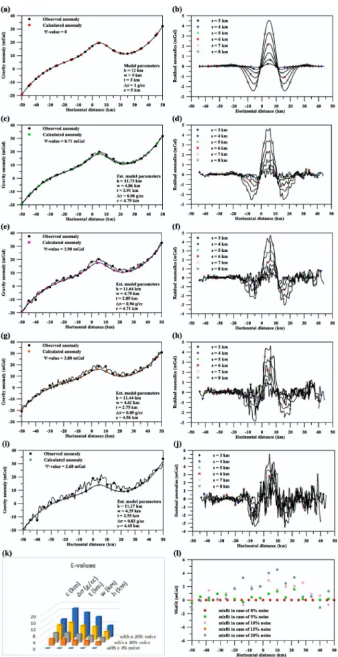
Firstly, a noise-free (0%) gravity anomaly profile of a two- dimensional thin sheet model (Fig. 2a). This anomaly exposed to the second moving average method to exclude the effect of the regional field utilizing several window lengths (s ¼ 3, 4, 5, 6, 7, and 8 km) (Fig. 2b). After that, the particle swarm method is applied to achieve the thin sheet parameters (h, w, t, Δσ, and c) (Table 1). Table 1 shows the ranges of every parameter; the depth (h) is between 1 and 20 km, the width (w) is between 1 and 20 km, the thickness (t) is between 1 and 10 km, the density contrast (Δσ) is between 0.5 and 1.5 g=cc , and the origin location of the buried body is between 1 and 20 km. Besides, Table 1 displays the estimated results for each parameter at every s-value, the average value (φavg), uncertainty, percentage error (E), and the root

mean squared value (ψ), which reveals the misfit amongst the observed and the calculated anomalies. According to the results in Table 1 in this case, the E-values and ψ-value equal zero (Fig. 2k and l).

Secondly, in case of adding 5% random noise on the composite anomaly (Δg) (Fig. 2c), the second moving average method was used for the similar window lengths (s ¼ 3, 4, 5, 6, 7, and 8 km) to exclude the regional anomaly in this field (Fig. 2d). Moreover, it is interpreted by utilizing the particle swarm algorithm to assess the body parameters

(Table 1). In Table 1, the φavg-values for h, w, t, Δσ, and c are 11.73 0.13 km,

4.86 0.06 km, 2.91 0.04 km, 0.96 0.02 g=cc, and 4.79

0.07, the E-values are 2.21%, 2.90%, 3%, 4%, and 4.07% (Fig. 2k), respectively, and the ψ-value is 0.71 mGal. Besides, the misfit is figured in Fig. 2l.

Thirdly, we increased the level of noise to be 10% adding to the composite anomaly in equation (7) (Fig. 2e). Using the same procedures as above, the second moving averages residual anomalies are revealed in Fig. 2f and the results are tabulated and demonstrated in Table 1. From Table 1, the estimated φavg-values for h, w, t, Δσ, and c are 11.64 0.13 km, 4.79 0.05 km, 2.85 0.03

km, 0.94 0.02 g=cc, and 4.71 0.04, the E-values are 3.03%, 4.17%, 5.11%, 6%, and 5.87% (Fig. 2k), respectively. The correlation between the observed and the calculated is estimated (the ψ-value is 2.90 mGal). Also, the difference (residual) between them is drawn in Fig. 2l.

Fourthly, a 15% random noise data was added to the composite anomaly (Fig. 2g). For the similar s-values (s ¼ 3, 4, 5, 6, 7, and 8 km), the second moving average residual gravity anomalies are presented in Fig. 2h. By utilizing the particle swarm algorithm for these noisy data, the outcomes of the source parameters (h, w, t, Δσ, and c) are presented (Table 1). The inferred outcomes in Table 1 represent the fitting among the observed and calculated, i.e., the φavg-values for h, w, t, Δσ, and c are 11.44 0.08 km, 4.61 0.08 km, 2.75 0.06

km, 0.89 0.03 g=cc, and

4.56 0.04, the E-values are 4.67%, 7.83%, 8.44%, 10.33%, and 8.76% (Fig. 2k), respectively, and the ψ-value equals 2.80 mGal. The misfit amongst the observed and calculated anomalies are presented in Fig. 2l.

Lastly, more random noise data (20%) was added to the mention above composite anomaly (Fig. 2i). By applying the similar procedures declared above, the second moving average residual anomalies are presented in Fig. 2j and the results due to using the global particle swarm algorithm are also mentioned in Table 1. Table 1 shows that the estimated φavg-values for h, w, t,

Δσ, and c are 11.17 0.09 km, 4.39 0.08 km, 2.55 0.06 km, 0.83 0.04 g=cc, and 4.45 0.08, and the E- values are 6.89%, 12.07%, 14.89%, 17.33%, and 10.83% (Fig. 2k), respectively. The comparison between the observed gravity anomaly and the calculated are assessed (the ψ-value is 2.68 mGal). Also, the difference (residual) between them is drawn in Fig. 2l.

Finally, these achieved values for noise-free and noisy test cases for the two-dimensional thin sheet model express that the suggested combination methods between utilizing the second moving average method that eliminated the regional background and noise and the particle swarm optimization method, which estimate the model parameters are steady and robust. 4. The comparison between the suggested approach and the window curves method

We inspected the proficiency and robustness of the anticipated method by matching its solutions with those achieved by the window curves method (Abdelrahman et al., 2016). The main difference amongst the proposed method and the window curves method are summarized as the best-estimates of the model parameters (depth and width).

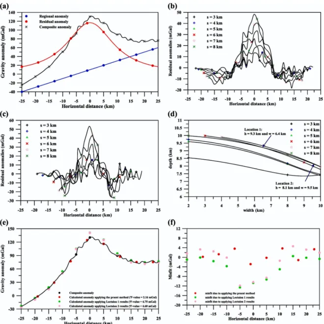
Fig. 3a shows a synthetic noisy (5% random noise impeded) for a two-dimensional thin sheet model of parameters: h ¼ 10 km, w ¼ 6 km, and profile length ¼ 50 km generated and containing a first-order regional background field applying the following equation:

(8) So, this composite gravity anomaly is subjected to the first moving average method that used in Abdelrahman et al. (2016) and the second moving average method that used in the suggested approach using several s-values (s ¼ 3, 4, 5, 6, 7, and 8 km) (Fig. 3b and c).

Firstly, we interpreted this gravity anomaly utilizing the window curves method (Abdelrahman et al., 2016) (Fig. 3d). Fig. 3d shows that two locations of intersect (two curves only) happens and no convergence at all. In other words, the results at the locations of intersection are summarized as follows: at location 1: h ¼ 9.3 km and w ¼ 6.4 km and at location 2: h ¼ 8.1 km and w ¼ 9.5 km.

For calculating the parameters (2GΔσtÞ, I developed the following form using the point xj ¼ 0: