doi: 10.3389/feart.2020.00301
Edited by: Aleksey Sadekov, The University of Western Australia, Australia Reviewed by: Jonathan Erez, The Hebrew University of Jerusalem, Israel Toshihiro Yoshimura, Japan Agency for Marine-Earth Science and Technology (JAMSTEC), Japan Alexandra V. Turchyn, University of Cambridge, United Kingdom *Correspondence: Volker Liebetrau vliebetrau@geomar.de †Present address: Rashid Rashid, Zanzibar University, Zanzibar, Tanzania
Specialty section: This article was submitted to Biogeoscience, a section of the journal Frontiers in Earth Science Received: 30 January 2019 Accepted: 26 June 2020 Published: 22 July 2020 Citation: Rashid R, Eisenhauer A, Liebetrau V, Fietzke J, Böhm F, Wall M, Krause S, Rüggeberg A, Dullo W-C, Jurikova H, Samankassou E and Lazar B (2020) Early Diagenetic Imprint on Temperature Proxies in Holocene Corals: A Case Study From French Polynesia. Front. Earth Sci. 8:301. doi: 10.3389/feart.2020.00301
Early Diagenetic Imprint on
Temperature Proxies in Holocene
Corals: A Case Study From French
Polynesia
Rashid Rashid1†, Anton Eisenhauer1, Volker Liebetrau1* , Jan Fietzke1, Florian Böhm1,
Marlene Wall1, Stefan Krause1, Andres Rüggeberg2, Wolf-Christian Dullo1,
Hana Jurikova1,3, Elias Samankassou4and Boaz Lazar5
1GEOMAR Helmholtz Centre for Ocean Research Kiel, Kiel, Germany,2Department of Geosciences, University of Fribourg,
Fribourg, Switzerland,3GFZ German Research Centre for Geosciences – Helmholtz Centre Potsdam, Potsdam, Germany, 4Department of Earth Sciences, University of Geneva, Geneva, Switzerland,5The Fredy & Nadine Herrmann Institute
of Earth Sciences, The Hebrew University of Jerusalem, Jerusalem, Israel
Coral-based reconstructions of sea surface temperatures (SSTs) using Sr/Ca, U/Ca and δ18O are important tools for quantitative analysis of past climate variabilities. However, post-depositional alteration of coral aragonite, particularly early diagenesis, restrict the accuracy of calibrated proxies even on young corals. Considering the diagenetic effects, we present new Mid to Late Holocene SST reconstructions on well-dated (U/Th: ∼70 yr to 5.4 ka) fossil Porites sp. collected from the Society Islands, French Polynesia. For few corals, quality pre-screening routines revealed the presence of secondary aragonite needles inside primary pore space, resulting in a mean increase in Sr/Ca ratios between 5-30%, in contrast to the massive skeletal parts. Characterized by a Sr/Ca above 10 mmol/mol, we interpret this value as the threshold between diagenetically altered and unaltered coral material. At a high-resolution, observed intra-skeletal variability of 5.4 to 9.9 mmol/mol probably reflects the physiological control of corals over their trace metal uptake, and individual variations controlled by CaCO3−precipitation rates. Overall, the Sr/Ca, U/Ca and δ18O trends are well correlated, but we observed a significant offset up to ± 7◦C among the proxies on derived palaeo-SST estimates. It appears that the related alteration process tends to amplify temperature extremes, resulting in increased SST-U/Ca and SST-Sr/Ca gradients, and consequently their apparent temperature sensitivities. A relative SST reconstruction is still feasible by normalizing our records to their individual mean value defined as1SST. This approach shows that 1SST records derived from different proxies agree with an amplitudinal variability of up to ± 2◦C with respect to their Holocene mean value. Higher1SST values than the mean SSTs (Holocene warm periods) were recorded from ∼1.8 to ∼2.8 ka (Interval I), ∼3.7 to 4.0 ka (Interval III) and before ∼5 ka, while lower1SST values (Holocene cold periods, Interval II and IV) were recorded in between. The ensuing SST periodicity of ∼1.5 ka in the Society Islands record is in line with the solar activity reconstructed from10Be and 14C production (Vonmoos et al., 2006), emphasizing the role of solar activity on climate variability during the Late Holocene.
Keywords: sea surface temperature (SST), chemical heterogeneities, scleractinian corals, diagenetic alterations, biomineralisation and calcification, late holocene climate
INTRODUCTION
Palaeo-climate reconstructions present a challenge for times beyond historical archives and instrumental records (Gagan et al., 2000; Grottoli, 2001). Among other natural archives typically used for climate reconstructions (e.g., tree rings, ice or sediment cores), scleractinian corals are considered one of the best recorders of environmental changes in shallow-water tropical oceans, offering a valuable window into past climatic oscillations in these regions (Beck et al., 1992;de Villiers et al., 1995;Min et al., 1995;McCulloch et al., 1996;Mitsuguchi et al., 1996;Shen et al., 1996;Schrag, 1999;Zinke et al., 2004). This is due to the uptake of trace element and isotope (TEI) signatures during biomineralisation processes accompanying coral growth, which act as sensitive chemical recorders – proxies – of environmental changes over the lifetime of the organism. Owing to their relatively high growth rates of up to several cm/year (Corrège, 2006), coral skeletons can provide continuous and undisturbed records with annual and even seasonal chronology spanning decades or centuries. These characteristics guarantee high temporal resolution down to a week or even better, as well as undisturbed records free of bioturbation (Corrège, 2006).
Geochemical proxy-based reconstructions have proven essential for reconstructing past seawater chemistry or temperature trends (Beck et al., 1992; Cohen and Hart, 2004; Corrège, 2006; Marchitto et al., 2010; Hathorne et al., 2011; Jurikova et al., 2019b). In particular, Sr/Ca, U/Ca and of δ18O signatures of corals have become important proxies
for deriving past sea surface temperature (SST) trends, a key climate parameter (Weber, 1973; de Villiers et al., 1995;
McGregor and Gagan, 2003; Yu et al., 2004; Hathorne et al., 2011). However, coral TEI records cannot simply be translated into environmental and/or climatic information; for each parameter (e.g., temperature) a species-specific calibration is required. This may be constrained from field studies or by analyses on coral material grown in culturing experiments under controlled laboratory conditions. Experiments have shown that the composition of biologically (i.e., coral-induced) and inorganically precipitated aragonite (CaCO3) may differ.
Specifically, coral Sr/Ca ratios are about 10 to 15% lower when compared to inorganic Sr/Ca ratios precipitated at the same temperature (Dietzel et al., 2004). This observation refers to the so-called “vital effect” and the strong physiological control of corals’ metabolism over the uptake of TEI from seawater upon CaCO3 precipitation. These processes are subject to numerous
studies dealing with biomineralisation and have to be considered prior to any palaeo-reconstructions (McConnaughey, 1989;
Cohen and McConnaughey, 2003;Cohen and Gaetani, 2010). A more general precondition that corals reliably record environmental conditions is that they preserve the primary TEI signals of the original skeletal aragonite (i.e., ‘closed system behavior’). This is not always the case because under natural conditions aragonite is thermodynamically unstable and hence susceptible to dissolution and recrystallization to secondary aragonite or calcite (diagenetic alteration). This process generates a reorganization of the chemical composition and may violate the ‘closed system behavior’ superimposing
and obscuring original TEI compositions. The latter process particularly affects Sr/Ca and U/Ca ratios since both tend to show considerably lower ratios in calcite than in aragonite (Reeder et al., 2000). In addition, exposure of fossil corals to meteoric water and groundwater causes dissolution of primary biological aragonite and re-precipitation of inorganic secondary calcite. Secondary inorganic aragonite precipitation is typical for marine diagenetic environments (Enmar et al., 2000). Dolomitization and cementation are processes further violating ‘closed system behavior’ (Land, 1973;Enmar et al., 2000;McGregor and Gagan, 2003; McGregor and Abram, 2008; Tucker and Wright, 2009) challenging the use of TEI in fossil scleractinian corals as a reliable TEI archive (Müller et al., 2001;Allison et al., 2007;McGregor and Abram, 2008;Nothdurft and Webb, 2009).
The magnitude and the type of diagenesis does not necessarily correlate with the age of a coral, but generally the type of environmental exposure, with coral species and skeletal porosity being the controlling factor for diagenesis (Dullo, 1986;Enmar et al., 2000; McGregor and Gagan, 2003; Hendy et al., 2007). For example, diagenesis can occur in a coral immediately post mortem, whereas fossil corals as old as 125 ka may remain unaffected by diagenetic alterations (Nothdurft and Webb, 2009). Studies have shown that precipitation of secondary aragonite within the pores of a coral skeleton is related to marine environments where the pores are saturated with seawater (Longman, 1980;Tribble et al., 1990). Replacement of aragonite by calcite, another diagenetic alteration, is mainly associated with fossil skeletons being exposed to a freshwater (Longman, 1980).
Palaeo-climate and palaeo-environmental reconstructions may be associated with uncertainties that are difficult to detect. For example, different phases of early diagenesis such as submarine secondary aragonite precipitation or dissolution of primary aragonite skeleton could lead to inaccuracies (Hendy et al., 2007; McGregor and Abram, 2008). This is because common methods like X-ray diffraction fail to distinguish between primary and secondary aragonite phases (earliest diagenetic phase). It has been suggested that even very small diagenetic changes might obscure any palaeo-climate estimates (McGregor and Gagan, 2003). For the Sr/Ca proxy, which has been found to be strongly affected by diagenesis (Sayani et al., 2011), it has been shown that the presence of ∼1% of calcite in the skeletal pores could result in about 1-2◦
C warmer SST estimates (McGregor and Gagan, 2003). About 2% of early diagenetic secondary aragonite is able to shift the SST estimates into cooler temperatures by 0.4 and 0.9◦
C (Allison et al., 2007). In contrast, theδ18O has been known to be less susceptible to diagenesis and also less impacted by calcite precipitation compared to the Sr/Ca proxy (McGregor and Gagan, 2003). Despite the recent increase in the use of coral skeletons in climatic and palaeo-oceanographic reconstructions, only few studies have focused on a detailed exploration of diagenetic imprints, their impacts on different geochemical signals, and strategies for extraction of reliable proxy information (e.g.,Gothmann et al., 2015).
The aim of the present study is to show the impact of early diagenetic imprints on SST proxies in Holocene corals. As a contribution to achieving the most precise palaeo-climatic reconstructions, we consider careful, high-resolution sampling
strategies, and compare areas affected by diagenesis with skeletal parts of original primary aragonite composition within single specimens. Finally, we attempt to constrain the Mid to Late Holocene climate history of the Society Islands, French Polynesia, using Sr/Ca, U/Ca ratios and δ18O isotopes from fossilPorites sp. corals that were exposed to subaerial conditions during Late Holocene sea level fall (Rashid et al., 2014).
MATERIALS AND METHODS
Study Area
The Society archipelago lies in the tropical South Pacific Ocean of French Polynesia between 17◦
520 S 149◦ 500 W and 15◦ 480 S 154◦ 500
W (Figure 1). The archipelago consists of more than ten islands lying along a distance of 720 km from southeast to northwest of the area (Duncan and McDougall, 1976;
Montaggioni, 2011). The islands are of volcanic origin formed by a hotspot (Teahiti’a-Mehetia), which is currently located around the Mehetia region as the Pacific plate moves over the hotspot in a northwest direction (Gripp and Gordon, 1990). They are characterized by extended fossil reef platforms, exposed above present sea level (Rashid et al., 2014). The geochronology of these islands is well established in the literature, with the ages of the islands increasing in a northwest direction as they move away from the hotspot; e.g., Mehetia (< 1 Ma), Tahiti (1.67–0.25 Ma), Moorea (2.15–1.36 Ma), Huahine (3.08–2.06 Ma), Raiatea (2.75– 2.29 Ma), Tahaa (3.39–1.10 Ma), Bora Bora (3.83–3.10 Ma) and Maupiti (5 Ma) (Duncan and McDougall, 1976; Duncan et al., 1994;White and Duncan, 1996;Blais et al., 1998, 2000;Guillou et al., 2005).
The climate of the Society Islands is tropical with two main seasons. The austral summer from November to April is the warm and rainy season, with relatively high average SSTs between 28◦
C and 29◦
C (Delesalle et al., 1985; Boiseau et al., 1998). Heavy rains mostly occur during December and January, principally affecting the coastal areas, with average rainfalls about ∼2750 mm/year (Cabioch et al., 1999). The austral winter from May to October is marked by low SSTs averaging between 23◦
C and 25◦
C and rarely dropping below 19◦
C (Delesalle et al., 1985). The tides are semi-diurnal with a mean amplitude of 0.5 m (Seard et al., 2011), and trade winds blow from East (South-East) and North-East direction.
Coral Sampling
In situ fossil Porites sp. corals were collected between −1.5 m below present mean sea level (bpmsl) and ∼1.8 m above the present mean sea level (apmsl) using hammer and chisel from the exposed shores of Moorea, Huahine and Bora Bora Island (Figure 1), French Polynesia in 2009 (seeRashid et al., 2014for further details). The samples were cut into ∼1 cm thick slabs parallel to the growth axis of coral skeleton visually selecting pristine areas for further processing. Selected samples were rinsed several times with deionized water and dried in a clean laminar floor hood under room temperature (∼20◦
C) for about 24 to 36 h. After drying, a diamond saw was used to cut out small cubes (∼1 cm3) from the distinct growth layers of the coral
(Figure 2). Greatest care was taken during the preparation of each subsample in order to avoid sampling of material of different ages. Subsequently, each cube was equally divided into two parts. One part was cut into small chips and placed in Teflon beakers with deionized water for ultra-sonification. The chips were then dried on a hot plate at 35◦
C for about 12-24 h. Using a mortar and a pestle, they were gently ground into a homogeneous powder, which was then used for X-ray diffraction (XRD) and geochemical analyses. The second half of the cube was used for microscopic observations (to evaluate any visible diagenetic alterations such as e.g., infillings, secondary precipitates) and high-spatial resolution geochemical analyses including electron microprobe mapping and micro-milling for further solution-based analyses.
Investigation of Early Diagenetic
Alteration: X-Ray Diffraction (XRD) and
Microscopic Observations
Detection and quantification of mineralogy of powdered samples in terms of aragonite or Mg-calcite was done using X-ray diffraction (XRD; ‘D8 Discover’ Bruker AXS) at Kiel University as described inAlKhatib and Eisenhauer (2017)andKrause et al. (2019). Briefly, samples were analyzed in a 22-range from 4◦
to 90◦
with a step size of 0.007◦
and counting time 1.5 s/step using a Cu X-ray radiation source. Software evaluation was done by High Score Plus Version 3.0d (3.0.4) by PANalytical. The XRD detection limit for aragonite and calcite is 2.9 and 0.9 mol.%, respectively (Kontoyannis and Vagenas, 2000).
Microscopic observations of the solid counterparts (the second sample cubes which were the mirror images of the crushed samples, as described in section “Coral Sampling”) for identification of any potential diagenetic alterations defined by the presence of infills or a distinct rim around the pores were carried out using an epi-fluorescence microscope (type: Zeiss Axio Imager.M2; camera: Zeiss AxioCam MRm Rev.3; light source: HXP 120 V (D); and objective: EC Plan-Neofluar 10x/0.3 M27) at GEOMAR, Kiel. For imaging we used the DAPI filter set with excitation of 350/50 nm and emission of 460/50 nm. Complementary high-resolution imaging was carried out on a ZEISS Ultra Plus Scanning Electron Microscope (SEM) at the GFZ, Potsdam (employing the In-lens & SE-Detector for high-resolution and Annular Backscatter Detector (AsB) for material contrast).
Geochemical Analyses of Bulk Samples
(Well-Preserved)
Bulk sample analyses were carried out only on samples with no detectable traces of calcite from XRD analysis. These measurements were performed using Varian 720-ES Inductively Coupled Plasma Optical Emission Spectrometry (ICP-OES) at GEOMAR, Kiel. Respective element emission signals were simultaneously collected and subsequently drift-corrected by sample-standard bracketing method done by measuring the reference material JCp-1 after every two samples, following the approach taken in previous studies (Schrag, 1999; de Villiers et al., 2002). The JCp-1 standard was prepared by
FIGURE 1 | (A) Present mean Sea Surface Temperature (SST) distribution in the Pacific region, with the location of French Polynesia indicated (where the Society Islands are located); (B) a close-up map of Society Islands where samples were collected.
the Geological Survey of Japan by homogenizing a massive Porites sp. sample (Okai et al., 2002), which Sr/Ca ratio is well-known from long-term inter-laboratory comparisons (Hathorne et al., 2013). The sample solution was prepared by dissolving approximately 10–30 mg of coral powder in 10 ml of 2% ultrapure HNO3. The working solution was prepared by dilution
of the sample solution with 2% HNO3 to a Ca concentration
of ∼25 ppm. An internal Indium standard was added to each sample in order to monitor any potential matrix effects and to correct for machine-induced drifts. Over the entire measurement period of 3 days, the average Sr/Ca ratio of the JCp-1 standard was 8.7 ± 0.1 mmol/mol (2σ, n = 13). This is in agreement with the certified Sr/Ca of Hathorne et al. (2013) and also agrees reasonably well with the average value of 8.9 ± 0.2 mmol/mol measured in this study using ICP-MS Quadrupole.
The U/Ca ratio was analyzed on ICP-MS Quadrupole at GEOMAR, Kiel using the same solution and standards as prepared for the ICP-OES. Similar to Sr/Ca, all measured U/Ca ratios were also normalized to the inter-laboratory JCp-1 standard results ofHathorne et al. (2013). The average U/Ca for JCp-1 was 1.18 ± 0.09µmol/mol (2σ, n = 13).
Oxygen isotope analyses were carried out following the standard procedures for carbonate samples at GEOMAR, Kiel. For this, ∼100 µg of homogeneous coral powder was reacted in a water-free phosphoric acid in an automated carbonate device “Carbo Kiel” (Thermo Fischer Scientific Inc.) at 73◦
C. The δ18O isotope ratios were measured on a MAT 253 mass
spectrometer (Thermo Fischer Scientific Inc.) and are expressed as deviations in per mille relative to the Vienna-PeeDee Belemnite (VPDB) standard. The external precision forδ18O throughout the analyses was ± 0.09h (2σ, n = 30).
Geochemical Analyses of Micro-Milled
(Sub)Samples (Altered)
Skeletal parts affected by early diagenetic alteration were primarily micro-milled to collect carbonate powder. Micro-milling as well as all further geochemical analyses were carried out at GEOMAR, Kiel. We used a binocular-based computer-controlled New Wave research micro-mill applying the following parameters: depth per pass of 5 µm, number of passes 10, scan speed of 10 µm/s, with the plunge speed of 25 µm/sec. Using this method, we were able to carefully collect carbonate powder from primary massive skeletal parts, and also along the porous parts where secondary diagenetic infillings were detected. Note that the porous parts may partly include some traces of the massive parts, as the secondary aragonite needles were too small to be sampled alone. Well-preserved samples were also included for a comparison. After micro-milling, the samples were prepared for electron microprobe measurements (EMP) and then polished.
In contrast to bulk samples, the micro-milled samples deemed as altered by early diagenesis were measured for Sr/Ca on an ICP-MS Quadrupole. The sample preparation and analytical procedures were the same as on the ICP-OES (as detailed in section “Geochemical Analyses of Bulk Samples (Well-Preserved)”). The measured Sr/Ca ratios are presented normalized to JCp-1, and the mean JCp-1 value determined on the ICP-MS Quadrupole was 8.864 ± 0.205 mmol/mol (2σ, n = 12), in a good agreement with the certified value of 8.838 ± 0.009 mmol/mol (Hathorne et al., 2013).
Electron microprobe mapping (EMP; JXA- 8200 JEOL) was used to investigate micrometer-scale high-resolution Sr/Ca variations within primary and secondary skeletal parts (as
FIGURE 2 | Photographs (A1–C1panels), light microscope (A2–C2), backscatter (A3–C3) and scanning electron microscope (A4–C4) images of the selected coral sample examples: (A) H-Tai-2; (B) HM4; and (C) WL1. Photographs show the retrieved samples from the field and the coral sampling approach during which small cubes were cut out. Diagenetic alterations are already visible from the light microscope images in the samples H-Tai-2 (A) and HM4 (B) as secondary aragonite needles precipitated within skeletal voids (indicated by black arrows), with the pores and needles being comparatively larger in the sample H-Tai-2 than in HM4. The third sample WL1 (C) is considered pristine as no secondary aragonite needles were found within the pores. Position of the EMP analyzed areas (as in Figure 5) is indicated in the backscatter images with solid line red rectangles, and dashed line red rectangles indicate the position of the close up images from scanning electron microscope (SEM; bottommost panels).
described in Jurikova et al., 2019a). The EMP maps were obtained by wavelength dispersive spectrometry mode measuring simultaneously Sr (La, TAP) and Ca (Ka, PETJ). Briefly, the electron beam was focused to a spot size of 2µm, accelerating voltage set to 15 kV and beam current to 100 nA. A step size of 2µm and an accumulation time of 10 ms were used, along with the map repeated to gather 5 accumulations of the selected area. Standards (Calcite, Volcanic glass – VG-2 as well as Kan1 and Strontianite) were measured before and after mapping the sample to convert raw intensities into Sr/Ca ratios.
Microprobe Sr/Ca maps were used to investigate Sr/Ca variations by line analysis. The lines span over different skeletal regions with a step size of 2µm. However, each point reflects the average of 20 adjacent pixels in horizontal or vertical direction. In each map, we consider values from lines passing the massive part of a skeleton only. This was then compared with a line starting from the massive part and crossing the porous parts where the secondary needles were observed.
Chronology
Chronology of the coral samples used in this study was established as detailed in Rashid et al. (2014). In summary, measurements of U and Th isotope ratios were done using a multistatic and multi-ion-counting MC-ICP-MS following the method of Fietzke et al. (2005). We used a mixed spike (233U/236U/229Th) calibrated for concentration measurements using NIST-SRM 3164 (U) and NIST-SRM 3159 (Th), as well as against CRM-145 uranium standard solution (NBL-112A) for U isotopic composition and against a secular equilibrium standard (HU-1) for the precise determination of 230Th/234U activity ratios. The total procedural blanks were between 0.5-1 pg for Th and 10-20 pg for U, within the range of typical values for this method and our laboratory (Fietzke et al., 2005). The ages of samples used in this study are provided in Tables 1, 2.
RESULTS AND DISCUSSION
Diagenetic Alterations and Coral Skeletal
System Behavior
Our XRD results indicate that out of 55 samples, four samples contained detectable amounts of calcite (CM3: 3%, WL2: 3%, H-Tai-4: 7%, and HV-3A: 12%); therefore, these samples were omitted from the SST estimates as these recrystallization criteria violate the ‘closed system behaviour’ (see section “INTRODUCTION” for further details). For all the other samples aragonite presented the dominant CaCO3-polymorph, with any
calcite contribution being below the detection limit.
Microscopic observations revealed the presence of secondary aragonite needles within the skeletal voids in two samples (although by XRD deemed not recrystallised to calcite) – H-Tai-2 (Age: 3.1H-Tai-2 ± 0.03 ka) and HM4 (Age: 1.55 ± 0.0H-Tai-2 ka; Figure 2). The H-Tai-2 (Figure 2A) showed few large pores filled with aragonite needles of ∼10-50 µm in length. In the sample HM4 (Figure 2B) small pores were more abundant filled with comparatively shorter needles on the order of ∼5-10µm. Differences in the needle size probably reflect the gradual
build-up of secondary aragonite with age, or alternatively an increased amount of pore water percolating through skeletons with larger volume of pores (Enmar et al., 2000). For comparison, we show the image of sample WL1 (1.82 ± 0.02 ka), which still exhibited the original (well-preserved) skeletal structure (Figure 2C). These three samples were selected as examples for further investigation of early diagenetic effects on the presented geochemical proxies, discussed in detail onwards. We stress, however, that any final palaeo-climatic interpretations are based on corals deemed as well-preserved.
Geochemical Composition of Bulk
Samples
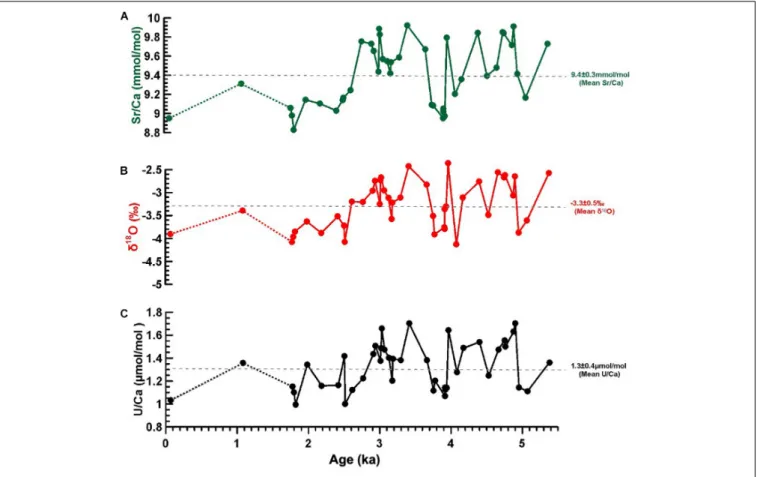
The results of Sr/Ca, δ18O, and U/Ca analyses together with the palaeo-SST reconstructions are summarized in Table 1 and shown in Figure 3 (all values are presented with 2σ standard deviation). The Sr/Ca ratio ranged between 8.83 ± 0.01 mmol/mol and 9.92 ± 0.02 mmol/mol corresponding to the average ratio of 9.4 ± 0.3 mmol/mol. The Sr/Ca ratios of two samples H-Tai-2 and HM4 were 10.14 ± 0.03 mmol/mol and 10.06 ± 0.03 mmol/mol, respectively. In these two samples, secondary diagenetic carbonate infill within the skeletal pores was detected by microscopic observations and thus these samples were excluded from SST estimates. The δ18O values varied between −4.13 ± 0.03 h and −2.35 ± 0.05 h, with an average value of −3.3 ± 0.5h. The U/Ca ratios ranged between 0.99 ± 0.02µmol/mol and 1.70 ± 0.02 µmol/mol corresponding to an average ratio of 1.3 ± 0.4µmol/mol. Sr/Ca, δ18O and U/Ca
trends were significantly correlated (Sr/Ca andδ18O: R2= 0.99,
n = 43, p < 0.005; U/Ca and Sr/Ca: R2= 0.98,n = 43, p < 0.005; U/Ca andδ18O: R2= 0.98,n = 43, p < 0.005).
Proxy Calibration
The δ18O-SST estimates were derived using the calibration equation by Boiseau et al. (1998)for modern Porites sp. from Moorea Island. The calibration equation is represented by a linear regression equation and rearranged for SST values as follows:
(1) SST (◦
C) = −4.35 ×δ18O (h VPDB) + 8.00
The Sr/Ca-SST estimates were based on the calibration equation for Porites sp. from Moorea Island (Cohen and Hart, 2004):
(2) SST (◦
C) = −3.58 × Sr/Ca (mmol/mol) + 58.93
For U/Ca-SST estimation we used the calibration equation of
Min et al. (1995)forPorites sp. from Tahiti Island: (3) SST (◦
C) = −18.40 × U/Ca (µmol/mol) + 45.00
Calculated SSTs are provided in Table 1. Note that the uncertainties on the reported SST estimates are based on the analytical uncertainties only.
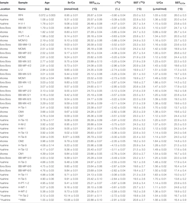
TABLE 1 | Sampling locations, age (ka), Sr/Ca ratios (mmol/mol),δ18O (
h), and U/Ca (µmol/mol), together with their reconstructed SSTs (◦C).
Sample Sample Age Sr/Ca SSTSr/Ca δ18O SSTδ18O U/Ca SSTU
/Ca
Location Name (ka) (mmol/mol) (◦C) (
h) (◦C) (µmol/mol) (◦C) Moorea RP4 0.072 ± 0.003 8.95 ± 0.01 26.87 ± 0.04 −3.90 ± 0.04 25.0 ± 3.3 1.03 ± 0.02 26.0 ± 0.3 Huahine HM5 1.08 ± 0.02 9.31 ± 0.02 25.57 ± 0.06 −3.39 ± 0.05 22.8 ± 3.0 1.36 ± 0.02 20.0 ± 0.4 Huahine H-V-1 1.78 ± 0.01 9.06 ± 0.02 26.48 ± 0.08 −4.07 ± 0.01 25.7 ± 3.4 1.15 ± 0.03 23.8 ± 0.5 Bora Bora BB-MX 7/2 1.79 ± 0.03 8.98 ± 0.01 26.77 ± 0.03 −3.97 ± 0.05 25.2 ± 3.3 1.10 ± 0.07 24.7 ± 1.3 Moorea WL1 1.82 ± 0.02 8.83 ± 0.01 27.29 ± 0.04 −3.85 ± 0.04 24.7 ± 3.3 0.99 ± 0.02 26.7 ± 0.4 Huahine H-PT-1-A 1.98 ± 0.02 9.14 ± 0.01 26.18 ± 0.04 −3.63 ± 0.04 23.8 ± 3.1 1.34 ± 0.01 20.3 ± 0.2 Moorea MCM10 2.19 ± 0.02 9.10 ± 0.02 26.32 ± 0.06 −3.88 ± 0.04 24.9 ± 3.3 1.16 ± 0.01 23.7 ± 0.3 Bora Bora BB-MM-13 2.42 ± 0.02 9.03 ± 0.01 26.58 ± 0.02 −3.52 ± 0.01 23.3 ± 3.0 1.16 ± 0.03 23.6 ± 0.5 Moorea MCM5 2.51 ± 0.02 9.14 ± 0.02 26.18 ± 0.06 −3.72 ± 0.02 24.2 ± 3.2 1.42 ± 0.02 18.9 ± 0.4 Bora Bora BB-MP-3/2 2.52 ± 0.03 9.17 ± 0.01 26.10 ± 0.04 −4.08 ± 0.04 25.7 ± 3.4 1.00 ± 0.01 26.6 ± 0.2 Moorea MCM2 2.61 ± 0.02 9.24 ± 0.01 25.82 ± 0.05 −3.20 ± 0.04 21.9 ± 2.9 1.12 ± 0.02 24.4 ± 0.3 Bora Bora BB-MX-3/2 2.77 ± 0.02 9.75 ± 0.04 23.99 ± 0.13 −3.20 ± 0.04 21.9 ± 2.9 1.23 ± 0.01 22.5 ± 0.3 Bora Bora BB-MP-4/2 2.91 ± 0.02 9.73 ± 0.01 24.08 ± 0.05 −2.96 ± 0.04 20.9 ± 2.8 1.43 ± 0.02 18.6 ± 0.3 Moorea LI-2 2.94 ± 0.03 9.65 ± 0.03 24.35 ± 0.09 −2.74 ± 0.03 19.9 ± 2.7 1.51 ± 0.03 17.3 ± 0.5 Bora Bora BB-MX-5/3 3.01 ± 0.03 9.44 ± 0.02 25.12 ± 0.08 −3.25 ± 0.04 22.1 ± 3.0 1.37 ± 0.03 19.7 ± 0.5 Moorea MCM1 3.02 ± 0.04 9.89 ± 0.01 23.52 ± 0.03 −2.73 ± 0.03 19.9 ± 2.7 1.49 ± 0.02 17.6 ± 0.4 Bora Bora BB-MX-1/2 3.03 ± 0.02 9.83 ± 0.02 23.73 ± 0.07 −2.67 ± 0.04 19.6 ± 2.7 1.66 ± 0.01 14.5 ± 0.2 Moorea LI-4 3.07 ± 0.02 9.57 ± 0.03 24.65 ± 0.11 −2.95 ± 0.03 20.8 ± 2.8 1.47 ± 0.01 17.9 ± 0.3 Bora Bora BB-MP-2/2 3.13 ± 0.02 9.55 ± 0.01 24.73 ± 0.05 −3.12 ± 0.04 21.6 ± 2.9 1.40 ± 0.04 19.2 ± 0.8 Bora Bora BB-MX-5/1 3.18 ± 0.02 9.42 ± 0.02 25.19 ± 0.08 −3.57 ± 0.04 23.5 ± 3.1 1.20 ± 0.02 22.8 ± 0.4 Bora Bora BB-MX-6/3 3.18 ± 0.03 9.54 ± 0.03 24.77 ± 0.09 −3.22 ± 0.04 22.0 ± 2.9 1.39 ± 0.03 19.3 ± 0.5 Bora Bora BB-MX-4/2 3.29 ± 0.02 9.59 ± 0.02 24.58 ± 0.09 −3.11 ± 0.04 21.5 ± 2.9 1.38 ± 0.02 19.6 ± 0.3 Huahine H-Tai-1 3.41 ± 0.02 9.92 ± 0.02 23.38 ± 0.07 −2.42 ± 0.03 18.5 ± 2.6 1.70 ± 0.02 13.7 ± 0.3 Moorea CM4 3.66 ± 0.03 9.67 ± 0.02 24.28 ± 0.07 −2.82 ± 0.06 20.3 ± 2.9 1.38 ± 0.01 19.6 ± 0.2 Moorea CM7 3.76 ± 0.04 9.09 ± 0.03 26.36 ± 0.09 −3.51 ± 0.02 23.3 ± 3.1 1.12 ± 0.01 24.4 ± 0.2 Huahine H-Tai-10 3.78 ± 0.17 9.08 ± 0.03 26.39 ± 0.09 −3.91 ± 0.02 25.0 ± 3.3 1.20 ± 0.01 22.9 ± 0.3 Huahine H-M-2 3.92 ± 0.02 8.95 ± 0.01 26.86 ± 0.04 −3.75 ± 0.01 24.3 ± 3.2 1.07 ± 0.01 25.3 ± 0.3 Huahine H-M-1 3.92 ± 0.04 9.05 ± 0.01 26.51 ± 0.04 −3.79 ± 0.03 24.5 ± 3.2 1.12 ± 0.02 24.3 ± 0.4 Huahine H-Tai-13 3.92 ± 0.05 9.02 ± 0.02 26.63 ± 0.07 −3.36 ± 0.03 22.6 ± 3.0 1.14 ± 0.03 24.0 ± 0.6 Huahine H-Tai-8 3.94 ± 0.05 8.971 ± 0.005 26.79 ± 0.02 −3.30 ± 0.03 22.4 ± 3.0 1.14 ± 0.01 24.0 ± 0.2 Moorea CM2 3.96 ± 0.03 9.79 ± 0.02 23.85 ± 0.07 −2.35 ± 0.05 18.2 ± 3.0 1.64 ± 0.02 14.8 ± 0.3 Huahine H-Tai-9 4.08 ± 0.14 9.20 ± 0.02 25.96 ± 0.08 −4.13 ± 0.03 25.9 ± 3.4 1.28 ± 0.01 21.5 ± 0.3 Huahine H-Tai-12 4.17 ± 0.07 9.36 ± 0.02 25.40 ± 0.07 −3.11 ± 0.07 21.5 ± 3.0 1.49 ± 0.03 17.6 ± 0.6 Moorea CM1 4.39 ± 0.04 9.84 ± 0.02 23.66 ± 0.05 −2.76 ± 0.04 20.0 ± 2.7 1.54 ± 0.03 16.7 ± 0.5 Bora Bora BB-MP-5/3 4.53 ± 0.02 9.39 ± 0.01 25.28 ± 0.04 −3.49 ± 0.04 23.2 ± 3.1 1.25 ± 0.03 22.0 ± 0.6 Huahine H-Tai-3 4.66 ± 0.05 9.48 ± 0.06 24.97 ± 0.21 −2.55 ± 0.03 19.1 ± 2.6 1.48 ± 0.02 17.9 ± 0.4 Bora Bora BB-MP-6/6 4.75 ± 0.02 9.85 ± 0.02 23.64 ± 0.06 −2.67 ± 0.04 19.6 ± 2.7 1.56 ± 0.02 16.4 ± 0.4 Bora Bora BB-MP-6/5 4.76 ± 0.03 9.84 ± 0.01 23.69 ± 0.04 −2.62 ± 0.04 19.4 ± 2.7 1.50 ± 0.02 17.4 ± 0.4 Huahine H-Tai-11 4.88 ± 0.06 9.71 ± 0.01 24.13 ± 0.05 −3.06 ± 0.05 21.3 ± 2.9 1.63 ± 0.04 15.0 ± 0.7 Huahine H-Tai-5 4.90 ± 0.06 9.91 ± 0.03 23.42 ± 0.10 −2.64 ± 0.03 19.5 ± 2.6 1.70 ± 0.01 13.6 ± 0.2 Huahine H-PT-1-2 4.95 ± 0.02 9.41 ± 0.02 25.21 ± 0.07 −3.87 ± 0.08 24.8 ± 3.4 1.14 ± 0.03 23.9 ± 0.5 Huahine H-MT-1 5.07 ± 0.05 9.16 ± 0.02 26.10 ± 0.06 −3.61 ± 0.03 23.7 ± 3.1 1.11 ± 0.01 24.6 ± 0.2 Huahine H-MT-2 5.38 ± 0.03 9.73 ± 0.03 24.08 ± 0.11 −2.58 ± 0.03 19.2 ± 2.6 1.36 ± 0.01 19.9 ± 0.2 **Huahine **H-Tai-2 3.12 ± 0.03 10.14 ± 0.03 22.61 ± 0.11 −2.72 ± 0.02 19.8 ± 2.6 1.54 ± 0.03 16.7 ± 0.5 **Huahine **HM4 1.55 ± 0.02 10.06 ± 0.03 22.88 ± 0.10 −2.91 ± 0.02 20.6 ± 2.7 1.56 ± 0.05 16.4 ± 0.9
**Indicates samples affected by early diagenesis (samples having secondary aragonite precipitates), these samples were not used for SST estimates.
Early Secondary Diagenesis and Its
Effects on Sr/Ca
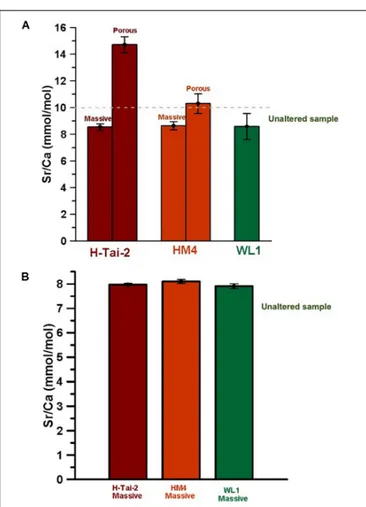
Micro-mill based sampling was applied to coral specimens affected by early diagenetic alterations in order to compare
the Sr/Ca composition of the massive, and the porous parts where the aragonite needles were found (Figure 4). For H-Tai-2, the sample originating from the massive part of the primary skeleton had a Sr/Ca ratio of 9.7 ± 0.3 mmol/mol, while the two samples from porous parts showed slightly increased
TABLE 2 | Sample name, Age (ka), the1SST (SST–Mean SST), weighted mean from each 1SST proxy record and a three-point running mean.
Sample Age SSTSr/Ca-MV SSTδ18O-MV SSTU/Ca-MV Normal Weighted 3 Point Running
Name (ka) (◦
C) (◦
C) (◦
C) Mean Mean Mean
*RP4 0.072 ± 0.003 1.65 ±0.20 2.77 ± 0.32 5.25 ± 0.62 3.22 2.60 ± 0.64 − *HM5 1.08 ± 0.02 0.35 ± 0.20 0.56 ± 0.34 −0.67 ± 0.63 0.08 0.25 ± 0.22 − H-V-1 1.78 ± 0.01 1.26 ± 0.20 3.52 ± 0.30 3.10 ± 0.65 2.63 2.31 ± 0.40 − BB-MX 7/2 1.80 ± 0.03 1.55 ± 0.20 3.06 ± 0.34 4.01 ± 0.88 2.87 2.35 ± 0.46 2.51 WL1 1.82 ± 0.02 2.07 ± 0.20 2.55 ± 0.32 5.98 ± 0.63 3.54 2.87 ± 0.73 2.05 H-PT-1-A 1.98 ± 0.02 0.96 ± 0.20 1.58 ± 0.32 −0.42 ± 0.61 0.71 0.93 ± 0.34 1.90 MCM10 2.19 ± 0.02 1.10 ± 0.20 2.68 ± 0.32 2.99 ± 0.61 2.26 1.92 ± 0.35 1.45 BB-MM-13 2.42 ± 0.02 1.36 ± 0.20 1.11 ± 0.30 2.88 ± 0.66 1.78 1.51 ± 0.32 1.43 MCM5 2.51 ± 0.02 0.96 ± 0.20 1.98 ± 0.31 −1.78 ± 0.64 0.39 0.86 ± 0.65 1.65 BB-MP-3/2 2.52 ± 0.03 0.88 ± 0.20 3.53 ± 0.32 5.89 ± 0.61 3.43 2.57 ± 0.87 1.42 MCM2 2.61 ± 0.02 0.60 ± 0.20 −0.28 ± 0.33 3.66 ± 0.62 1.33 0.84 ± 0.69 1.00 BB-MX-3/2 2.77 ± 0.02 −1.23 ± 0.21 −0.26 ± 0.33 1.75 ± 0.61 0.08 −0.40 ± 0.53 −0.31 BB-MP-4/2 2.91 ± 0.02 −1.14 ± 0.20 −1.33 ± 0.33 −2.11 ± 0.62 −1.53 −1.36 ± 0.18 −1.17 LI-2 2.94 ± 0.03 −0.87 ± 0.21 −2.27 ± 0.32 −3.42 ± 0.66 −2.19 −1.75 ± 0.45 −1.11 BB-MX-5/3 3.01 ± 0.03 −0.10 ± 0.20 −0.06 ± 0.33 −1.01 ± 0.65 −0.39 −0.23 ± 0.18 −1.37 MCM1 3.02 ± 0.04 −1.70 ± 0.20 −2.34 ± 0.32 −3.07 ± 0.63 −2.37 −2.13 ± 0.24 −1.67 BB-MX-1/2 3.03 ± 0.02 −1.49 ± 0.20 −2.59 ± 0.33 −6.24 ± 0.61 −3.44 −2.64 ± 0.86 −1.99 LI-4 3.07 ± 0.02 −0.57 ± 0.21 −1.35 ± 0.32 −2.82 ± 0.61 −1.58 −1.22 ± 0.40 −1.51 BB-MP-2/2 3.13 ± 0.02 −0.49 ± 0.20 −0.63 ± 0.33 −1.51 ± 0.72 −0.88 −0.69 ± 0.19 −0.38 BB-MX-5/1 3.18 ± 0.02 −0.03 ± 0.20 1.35 ± 0.32 2.13 ± 0.63 1.15 0.77 ± 0.38 −0.15 BB-MX-6/3 3.18 ± 0.03 −0.45 ± 0.21 −0.19 ± 0.32 −1.37 ± 0.64 −0.67 −0.52 ± 0.21 −0.16 BB-MX-4/2 3.30 ± 0.02 −0.64 ± 0.20 −0.67 ± 0.33 −1.13 ± 0.62 −0.81 −0.73 ± 0.10 −1.51 H-Tai-1 3.41 ± 0.02 −1.84 ± 0.20 −3.67 ± 0.32 −7.02 ± 0.62 −4.18 −3.28 ± 0.91 −1.76 CM4 3.66 ± 0.03 −0.94 ± 0.20 −1.92 ± 0.36 −1.15 ± 0.61 −1.33 −1.26 ± 0.17 −0.99 CM7 3.76 ± 0.04 1.14 ± 0.21 1.08 ± 0.31 3.74 ± 0.61 1.99 1.56 ± 0.52 0.73 H-Tai-10 3.78 ± 0.17 1.17 ± 0.21 2.82 ± 0.31 2.17 ± 0.61 2.05 1.89 ± 0.28 1.91 H-M-2 3.92 ± 0.02 1.64 ± 0.20 2.13 ± 0.30 4.61 ± 0.62 2.80 2.29 ± 0.54 2.06 H-M-1 3.92 ± 0.04 1.29 ± 0.20 2.29 ± 0.32 3.61 ± 0.64 2.39 1.98 ± 0.41 1.88 H-Tai-13 3.92 ± 0.05 1.41 ± 0.20 0.42 ± 0.31 3.24 ± 0.66 1.69 1.37 ± 0.48 1.59 H-Tai-8 3.94 ± 0.05 1.57 ± 0.20 0.17 ± 0.32 3.32 ± 0.61 1.69 1.42 ± 0.52 −0.05 CM2 3.97 ± 0.03 −1.37 ± 0.20 −3.96 ± 0.36 −5.94 ± 0.62 −3.76 −2.92 ± 0.82 0.07 H-Tai-9 4.08 ± 0.14 0.74 ± 0.20 3.74 ± 0.32 0.78 ± 0.62 1.75 1.71 ± 0.55 −0.60 H-Tai-12 4.17 ± 0.07 0.18 ± 0.20 −0.69 ± 0.38 −3.08 ± 0.67 −1.19 −0.60 ± 0.61 −0.35 CM1 4.40 ± 0.04 −1.56 ± 0.20 −2.20 ± 0.33 −4.03 ± 0.65 −2.60 −2.16 ± 0.45 −0.74 BB-MP-5/3 4.53 ± 0.02 0.06 ± 0.20 0.96 ± 0.32 1.33 ± 0.67 0.78 0.55 ± 0.23 −1.10 H-Tai-3 4.66 ± 0.05 −0.25 ± 0.23 −3.09 ± 0.32 −2.85 ± 0.63 −2.06 −1.68 ± 0.55 −1.16 BB-MP-6/6 4.75 ± 0.02 −1.58 ± 0.20 −2.58 ± 0.33 −4.32 ± 0.63 −2.83 −2.35 ± 0.49 −2.08 BB-MP-6/5 4.76 ± 0.03 −1.53 ± 0.20 −2.80 ± 0.33 −3.30 ± 0.64 −2.54 −2.22 ± 0.32 −2.06 H-Tai-11 4.88 ± 0.06 −1.09 ± 0.20 −0.89 ± 0.34 −5.73 ± 0.68 −2.57 −1.75 ± 0.95 −2.12 H-Tai-5 4.90 ± 0.06 −1.80 ± 0.21 −2.70 ± 0.32 −7.07 ± 0.61 −3.86 −3.00 ± 0.97 −1.16 H-PT-1-2 4.95 ± 0.04 −0.01 ± 0.20 2.65 ± 0.39 3.23 ± 0.66 1.95 1.28 ± 0.64 −0.05 H-MT-1 5.07 ± 0.05 0.88 ± 0.20 1.50 ± 0.32 3.86 ± 0.61 2.08 1.58 ± 0.54 0.39 H-MT-2 5.38 ± 0.03 −1.14 ± 0.21 −3.00 ± 0.32 −0.77 ± 0.61 −1.64 −1.69 ± 0.39 −
Data indicated by * are plotted as separate points due to a missing data gap in between. As a consequence, a three-point running mean is not available from these points (as there are only two data points).
ratios of 10.5 ± 0.2 mmol/mol and 10.7 ± 0.05 mmol/mol. For HM4, similarly, the sample from the massive area had a Sr/Ca ratio of 9.9 ± 0.1 mmol/mol, whereas the two samples from the porous parts had a ratio of 10.1 ± 0.1 mmol/mol and of 10.1 ± 0.3 mmol/mol. For this sample, the composition of the porous and massive parts overlaps within error, most likely due to the very early stage of the secondary aragonite
precipitation, based on the relatively small needle size in HM4 when compared to H-Tai-2. Thus, it appears that the Sr/Ca of these needles is rather low and would not significantly impact any SST estimates. Note that, although our sampling strategy discriminates between porous vs. massive skeleton areas, the samples from the porous parts may contain small traces of the massive skeletal parts. In general, we observed a common trend
FIGURE 3 | (A) Sr/Ca; (B)δ18O; and (C) U/Ca series from the measured corals plotted against the corresponding ages. Dotted line in each of the series between ∼1–2 ka indicates time interval with only few data points, where the trend should not be considered confident. The gray dashed line represents the average value for each proxy.
with all samples from the massive parts tending to have Sr/Ca ratios below 10 mmol/mol, and those from the porous parts affected by early diagenetic imprints above 10 mmol/mol. This observation is also highly comparable to results from the altered bulk samples. We therefore propose the Sr/Ca of 10 mmol/mol as a threshold value for diagenetic alteration. We note that this threshold values is based on Porites sp. from Society Islands, and while potentially applicable beyond, should not be taken at a face value without prior validations when applying to other species and/or regions.
Diagenesis in terms of secondary aragonite precipitation can be expected to drive the original Sr/Ca signature of coral skeletons towards higher values by introducing new aragonite material with increased Sr/Ca that interferes with the primary signals, potentially distorting proxy reconstructions (McGregor and Gagan, 2003; Allison et al., 2007). For instance, about 2.5-3% of secondary aragonite precipitation within the skeletal voids found in our diagenetically influenced coral skeleton would shift the SST estimates derived from bulk samples towards cooler temperatures by 0.5-1.6◦
C. This estimate may be obtained by subtracting the bulk Sr/Ca values from the average Sr/Ca of the micro-milled samples, and then considering the deviation in SST from the SST-Sr/Ca calibration equation.
The observed differences in Sr/Ca of altered and non-altered samples can be explained in terms of inorganic and biologically induced precipitation. While during secondary precipitation inorganic aragonite formed from seawater builds up in the pores, the original biologically grown skeleton is influenced by physiological effects modifying the Sr/Ca ratio (Cohen et al., 2002;Cohen and Gaetani, 2010).
Electron microprobe analyses of H-Tai-2 (Figures 5A1−D1)
and HM4 (Figures 5A2−D2) revealed high Sr and Ca
concentrations around pore spaces and along aragonite needles, when compared to the massive parts of the coral skeleton. The well-preserved sample WL1 showed no variations in EMP-derived Sr/Ca of the skeleton (Figures 5A3−D3). Point analysis
(or spot analysis) of primary massive skeletal aragonite in sample H-Tai-2 gave an average Sr/Ca of 8.6 ± 0.2 mmol/mol, while the Sr/Ca was considerably higher of ∼14.7 ± 0.6 mmol/mol in the needles and pores (Figure 6). Conversely, the Sr/Ca in the massive, primary, skeletal areas was 8.7 ± 0.3 mmol/mol in HM4, with increased values of ∼10.3 ± 0.7 mmol/mol around the pores. While both H-Tai-2 and HM4 were affected by early diagenesis, the higher Sr/Ca ratio of H-Tai-2 (14.7 ± 0.6 mmol/mol), when compared to HM4 (10.3 ± 0.7 mmol/mol), is most likely due to larger pore size and longer secondary aragonite needles. For a reference, the Sr/Ca measured by EMP in the well-preserved
FIGURE 4 | Sr/Ca results from micro-mill based sampling in coral samples affected by diagenesis (H-Tai-2 and HM4). The sampling targeted two different skeletal phases – massive coral areas vs. porous parts. Light pink band indicates measurements below the threshold value of 10 mmol/mol. Data from a sample considered well-preserved based on microscope observations (WL1) is provided for comparison, laying below the defined threshold value.
FIGURE 5 | Electron microprobe (EMP) Sr and Ca concentration distribution maps in the studied coral samples. Panels (A1–D1) show the Ca, Sr, Sr/Ca, and Sr/Ca line analysis in the sample H-Tai-2, panels (A2–D2) in HM4, and (A3–D3) in WL1 sample. Note the shift towards higher elemental concentrations at the rims and within the aragonite needles in diagenetically altered samples. Positions of the line analyses are indicated within the EMP maps as white lines, with results presented in the right panels (D). Here, blue lines indicate single values and black lines the three-point running mean. Sr/Ca ratios from line analyses were obtained by dividing measured Sr content by Ca in the same cell along a line after calibration. Elemental content is given in weight percent in the EMP maps and in mmol/mol for Sr/Ca in the line analysis plots.
FIGURE 6 | Mean Sr/Ca ratios obtained from: (A) point analyses of the EMP maps comparing massive vs. porous parts (in sample WL1 only the massive part was measured), with the dashed line indicating the defined threshold value for diagenetic alterations; and (B) and from line analyses within the massive parts. Note that in order to obtain representative results multiple line analyses were placed in the target area of each specimen, and error bars indicate the standard error of the mean.
sample (WL1) was 8.6 ± 0.5 mmol/mol. Finally, we note that the EMP-Sr/Ca values in the porous areas of H-Tai-2 (up to ∼14.7 ± 0.6 mmol/mol) were higher than those obtained by the micro-milling approach. This can be attributed to the fact that the point analysis method takes into account pixels with secondary aragonite only (as seen in the EMP map), while the micro-mill based data may contain traces of primary aragonite due to the limited resolution of the sampling method.
Intra-Skeletal Sr/Ca Variabilities in
Primary Coral Aragonite
Despite decades of research and extensive literature, the origin of micro-scale Sr/Ca heterogeneities in coral skeletons is still debated. While Sr/Ca is generally accepted as a robust palaeo-SST proxy, at a high-resolution, corals have been found to exhibit large Sr/Ca heterogeneities, which are not temperature dependant. Such heterogeneities may be largely linked to the different skeletal structures and their biomineralisation mechanisms (i.e., centres of calcification, COCs vs. fasciculi). For
instance, fasciculi (deposited during the day) have been found to be enriched in Sr/Ca in comparison to COCs (deposited at night), with heterogeneities of both features therefore apparently reflecting short-term variations in calcification rates that influence the relative transport of Sr and Ca through the coral tissues (Allison and Finch, 2004). Similarly,Ferrier-Pagès et al. (2002)reported incorporation of Sr2+to be inversely correlated
to calcification rate, suggesting interactions between Ca2+ and Sr2+ions. In addition to physiological processes dominating on daily scales,Cohen and Sohn (2004), for example, documented periodic variations in Sr/Ca linked to tidal water level oscillations, which may be modulated through changes in zooxanthellae photosynthesis with available photosynthetically active radiation. Further metabolic processes, such as physiological regulation in the calcifying fluid, have been also considered an important driver of numerous TEI variations and may directly or indirectly contribute to micro-scale variations in Sr/Ca (e.g.,Sinclair, 2005;
D’Olivo et al., 2018;Jurikova et al., 2019b).
Using EMP line analyses, likewise, we found that on a sub-cm fine scale Sr/Ca is not homogeneously distributed in the preserved massive primary coral skeleton (Figures 5A–C), with variations between 5.4 mmol/mol and 9.9 mmol/mol. Line positions were chosen to cover the maximum natural Sr/Ca variability within the massive parts. Results show that observed variability remained below a Sr/Ca ratio of 10 mmol/mol. Therefore, this value was defined as the threshold for natural variability, and Sr/Ca (mmol/mol) exceeding 10 were ascribed to diagenetic changes. The average Sr/Ca values (Figure 5D) for all three samples (H-Tai-2, HM4 and WL1) are, however, highly consistent (7.98 ± 0.04, 8.10 ± 0.08, and 7.91 ± 0.10 mmol/mol, respectively) and overlap within error with data from point analyses of the massive parts shown in Figure 6.
Based on the line analyses, it is evident that at a high-resolution the relative amplitude as well as the overall trends are highly variable between the samples (Figure 5). Particularly noticeable is the difference between the sample H-Tai-2 with reduced amplitude in Sr/Ca (Figure 5D1), and samples HM4
(Figure 5D2) and WLI (Figure 5D3) with more variable values.
Taking into account the obvious presence of secondary needles close to the line transect in the H-Tai-2, it can be expected that even the massive part away from the pore would have been affected by diagenetic overprinting. This could perhaps explain the relatively homogenous Sr/Ca trends, however, the absolute values are difficult to reconcile with the micro-milled data that situate the diagenetic threshold at 10 mmol/mol, according to which we would expect overall higher values for H-Tai-2. This suggests that other factors than diagenesis are responsible for driving micro-scale Sr/Ca variations in fossil corals, and demonstrates that the massive skeletal parts might still preserve original geochemical signatures, even with the presence of secondary needles in the neighboring pore spaces.
Plausibly, the observed Sr/Ca variations could be caused by inter-specific differences, or attributed to different orientation of the line analyses with respect to the growth axis. Specifically, the less variable Sr/Ca from the line analysis of the H-Tai-2 sample, could potentially indicate that the growth direction runs vertically, although it is difficult to conclude whether this would
be from the bottom to the top, or vice versa (Figure 5A). In the second example, the sample HM4, the Sr/Ca heterogeneity along the horizontal axis might indicate vertical growth direction (Figure 5B), and finally in the sample WL1 the heterogeneity suggests horizontal growth direction (Figure 5C).
Furthermore, the relative distributions seem to be much more heterogeneous than the expected SST trends, which also points towards other than ambient seawater conditions as controls of the Sr/Ca trends at a high-resolution. Therefore, we conclude that the observed micro-scale heterogeneities likely result from a combination of non-equilibrium processes during crystals formation or biologically mediated variations in the calcifying fluid, which can be expected to be at least partially linked to growth, and hence the orientation to the growth axis. Regardless, as demonstrated by our combined Sr/Ca analyses, provided that a mean value for a skeletal part is taken (achievable by micro-milling or averaging EMP data within the massive skeletal parts for samples affected by early diagenesis, and by bulk measurements in pristine samples) the proxy relationship holds, a common observation for a vast number of proxies.
Multi-Proxy Comparison of Sea Surface
Temperature Reconstructions
(SST-Sr/Ca, SST-U/Ca, and SST-
δ
18O)
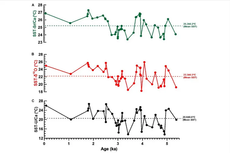
Using our geochemical data, a SST record from Mid Holocene (5.4 ka) to ∼70 years BP was reconstructed from well-preserved samples not affected by diagenesis (Table 1). The record shows a clear SST pattern of high and low temperatures recorded in the coral skeleton (Figure 7). The apparent palaeo-SST estimates derived from Sr/Ca ranged between 23.38 ± 0.07◦
C and 27.29 ± 0.04◦
C (with an average of 25.2 ± 0.2◦
C; SE: 1.3◦
C). Theδ18O based SSTs were systematically lower, ranging
between 18.2 ± 3.0◦
C to 25.9 ± 3.4◦
C (with a mean value of 22.3 ± 0.3◦
C; SE: 2.0◦
C). Lastly, estimates derived from U/Ca gave wider temperature ranges and more extreme SSTs varying between 13.6 ± 0.2◦ C and 26.7 ± 0.4◦ C (and with a mean value of 20.6 ± 0.6◦ C; SE: 3.9◦ C). This corresponds to a relative offset of 3.0 ± 0.2◦
C between SST-Sr/Ca SST-andδ18O,
1.5 ± 0.4◦
C forδ18O and U/Ca, and 4.5 ± 0.5◦
C between Sr/Ca and U/Ca. Although the absolute values differed significantly (based on a Student’s t-test; p < 0.0001), the relative trends remained similar for all three SST records. The offsets between the different calibrations and thus in the absolute reconstructed SSTs, however, suggest that the proxy-relationships are not as robust as previously thought, or at least their uncertainties are much larger than indicated in the literature.
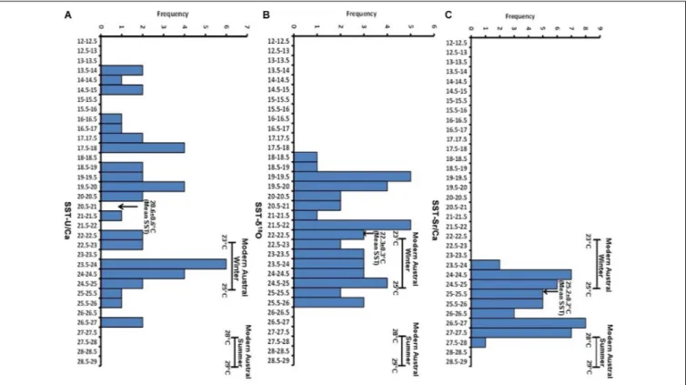
Concerning the statistical distribution of Sr/Ca-, U/Ca- and δ18O-derived SSTs we would expect to see a Gaussian-like
distribution around a given mean with distinct modern seasonal extreme values. However, from the histogram in Figure 8A it is evident that the Sr/Ca-STT data show a bimodal distribution, where the SSTs derived from low Sr/Ca ratios peak at about 23.5◦
C, closely corresponding to the long-term austral winter SST at the study site. The high austral summer temperatures of 28 to 29◦
C, however, are not reflected in reconstructed SSTs. Either such high SSTs were not common during the
Late Holocene, and hence the average SSTs are lower, or the Sr/Ca temperature calibration has a bias towards lower values by approximately 1◦
C. Alternatively, early diagenesis (i.e., precipitation of secondary aragonite, inconspicuous by our skeletal observations) overprinted the original signal resulting in higher Sr/Ca and hence systematically lower reconstructed temperatures. This can be tested by a back-envelope calculation, assuming a seawater Sr/Ca value of 8.541 mmol/mol and that secondary aragonite precipitates with a 15% higher partitioning coefficient than the coral aragonite, which implies a 20% contribution of secondary aragonite to the original skeletal material (e.g., Krause et al., 2019). Although we detected secondary aragonite built in the pores in two samples (see section “Early Secondary Diagenesis and Its Effects on Sr/Ca”), its distribution was not continuous, and secondary aragonite was completely absent in the massive areas of the coral. This implies that the massive parts follow, geochemically, a ‘closed system behavior’, and as based on our detailed assessment should not be affected by early diagenesis. However, potentially, post-mortem changes in Sr/Ca, even in the massive parts might still be possible, presumably driven by a simple ion exchange process during which lattice-bound Ca2+ions are exchanged for Sr2+ions from seawater. This would require the assumption that while seawater percolates through and diffuses into the coral, simultaneous exchange of ions occurs between the solid and liquid phases.
The δ18O-derived SST values also showed a bimodal distribution (Figure 8B), comparable to the Sr/Ca-SST values. Nonetheless, the δ18O-SST estimates appeared shifted to even
cooler temperatures than those derived from the Sr/Ca record. Moreover, the reconstructed maximum SSTs are about 3◦
C cooler than those expected for an austral summer today. Similar as for Sr/Ca this could point to proxy calibration uncertainties, or as previously postulated, post-mortem ion exchange processes with seawater. In particular for the latter, this could result in a bias towards lower temperatures, as seawater is relatively heavier in δ18O to a coral (and theδ18O-SST proxy relationship is inversely
correlated). In addition, a shift towards cooler conditions could be caused by secular changes in seawaterδ18O (δ18Osw) as a result
of evaporation or advection of18O-enriched waters (e.g.,Gagan et al., 1998; Stevenson et al., 2018). Given that our sampling location is influenced by the South Pacific Convergence Zone, which has been experiencing a freshening and warming trend since the 1850s (Dassié et al., 2014), an offset in the reconstructed Holocene SSTs could also be introduced through the use of a calibration based on recent specimens ad seawaterδ18O (rather
than those prior to 1850s). Furthermore, the shift of all proxies records towards lower SST values corresponds to the observation that the standard deviations of the SST-Sr/Ca, (25.2 ± 0.2◦
C; SE: 1.3◦ C), SST-δ18O (22.3 ± 0.3◦ C, SE: 2◦ C) and SST-U/Ca (20.6 ± 0.6◦ C; SE: 4◦
C) mean values increases as a function of the deviation from the modern mean value. This observation might potentially also indicate that the origin of the shift toward cooler temperature is the ion exchange with seawater rather than an inexact proxy-temperature calibration.
Similar to Sr/Ca and δ18O, the U/Ca-derived SSTs also
resulted in temperatures significantly below (average SST values: 20.6 ± 0.6◦
FIGURE 7 | Comparison of SSTs records for Mid to Late Holocene derived from: (A) Sr/Ca ratios; (B)δ18O values; and (C) U/Ca ratios. Dashed lines indicate the mean SST estimate for each proxy record.
values (Figure 8C). Following the approach applied above it may also be assumed that either the U/Ca-temperature calibration shows a distinct offset shifting the SST-U/Ca to lower temperatures, or that alternatively post-mortem U is taken up from the seawater percolating through the coral aragonite, thereby shifting the U/Ca-derived SST to even much cooler values than those expected from the modern seasonality.
In summary, while our pre-screening confirmed early diagenetic alterations in two specimens only (H-Tai-2 and HM4) detected by the presence of secondary aragonite in the pores, the massive parts of the skeleton and the great majority of our samples was deemed well-preserved, and thus assumed to follow ‘closed system behavior’. Nonetheless,Cuif and Dauphin (2005)
showed microstructural patterns of organic layers at a nanometer scale formed in the massive part of the skeleton that are related to the growth of the skeleton. After the death of a coral these organic layers might be exposed to microbial decomposition, which may give origin to micro-spaces or pathways in the massive parts of the coral skeleton. This could enable seawater to diffuse even into the massive coral areas, and favor secondary inorganic aragonite precipitation within these micro-spaces, probably also exchanging ions with the coral skeleton. This could potentially explain the observed discrepancies between
the temperature proxies, even in samples considered well-preserved. The amount of extra Sr and U added to the coral, however, appears to be constant rather than erratic in space and time, as otherwise it would be difficult to explain the strong correlation between the three proxies. The latter assumption thus offers the possibility to normalize the measured proxy values to their corresponding means, in order to further study second order variations in our proxy records rather than the absolute values.
Origin of the SST-Variations and Wider
Implications for the Late Holocene
Climate Change
Following the above approach to circumvent the problem of comparing absolute values we subtracted the mean SST values from the single values (Table 2) to obtain 1SSTs (Figure 9). These enable the comparison of the single record deviations from their respective mean values (Figure 9A). The three 1SST records are in a general agreement concerning the timing and phase, whereas the amplitudes differ substantially up to +6◦
C and −7◦
C for the U/Ca-derived 1SST. The δ18O-derived 1SST values
FIGURE 8 | Histogram plots showing the frequency of each proxy-SSTs in intervals of 0.5◦
C as a function of the corresponding absolute temperature; (A) U/Ca-SST, (B)δ18O-SST, and (C) Sr/Ca-SST. A general trend towards tailing of the values in direction of lower temperatures is visible. In particular, the recorded temperatures are lower than the present-day austral summer values and even tend to be lower than the modern austral winter values. Smallest temperature interval is recorded for the SST-Sr/Ca (28 to 23.5◦C) and largest for the SST-U/Ca (27 to 13.5◦C).
exhibit smaller variations restricted to the amplitudinal variations in between ± 4◦
C. For later comparison to different records we calculated a weighted average mean from the three temperature records and performed a three-point running mean in order to discard single excursions of high and low deviations from the mean value (blue curve of Figure 9A). The amplitudinal variation of the weighted mean curve (SST-all proxies) shows a reduced temperature range on the order of ± 2.4◦
C. Excluding the U/Ca record with highest amplitudinal extremes, the weighted mean leads to a decrease in the temperature variations down to the order of ∼2◦
C (Figure 8B).
The regional increase in temperatures from Mid Holocene to the modern periods has been suggested as on the order of ∼1.5◦
C in the North Pacific (Marchitto et al., 2010) and ∼2◦
C in the Eastern Pacific (Koutavas and Sachs, 2008), which is also in a good agreement with our estimates. However, our data show a SST pattern coinciding with four main time intervals, interval I (∼1.8 to ∼2.8 ka), interval II (∼2.8 to ∼3.7 ka), interval III (∼3.7 and 4.0 ka) and interval IV (∼4.0 to ∼4.9 ka). Interval II and IV show relatively low temperatures up to maximum ∼2.0◦
C below the average and interval I and interval III show temperatures up to ∼2◦
C higher than the long-term average (Figure 9B). Variations in the solar activity have contributed to climate change especially on longer time scales (Wanner et al., 2008) and besides atmospheric CO2 concentration it is probably
the most important factor controlling Earth’s temperature on non-astronomical and millennial time scales (Elsig et al., 2009; Hansen et al., 2013), which may also influence SST variabilities (Deser et al., 2010). Past solar variability can be reconstructed from cosmogenic 10Be and 14C records measured in the continental ice since they are produced in the upper part of the atmosphere as a direct function of solar activity. These isotope systems can be considered as proxies for the intensity of solar radiation (Bard and Frank, 2006; Wanner et al., 2008) and their variations are found to be in good agreement with our mean SST record (Figure 9C). In particular, we observe that the four main intervals of lower and higher temperatures correspond to periods of low and high solar activity, respectively. Furthermore, our SST patterns are similar in phase and amplitude to the general patterns of the solar activity. Solar activity variations are a global rather than a regional phenomenon hence solar activity also correlates with the ice dynamics of the important glaciated regions of the globe. For example, at ∼2.8 to 3.7 ka (interval II) and at ∼4.4 to 4.9 ka (interval IV) low temperature patterns correspond to times of glacial advances in several parts of the world, including the Alps, Scandinavia, Himalayas, Alaska, New Zealand and Patagonia (Grove, 2004; Thompson et al., 2006). At regional scale, this interpretation is also in agreement with the SST records from the Eastern Pacific where colder temperatures
FIGURE 9 | (A) Reconstructed1SSTs from Sr/Ca, δ18O, and U/Ca series plotted against age, including a mean weighted average of all1SST proxies (blue curve). Four intervals of alternating SSTs can be identified: two warm periods (where the SST is above the mean, intervals I and III) and cold intervals where the SST is below the mean (intervals II and IV); (B) reconstructed1SSTs from Sr/Ca and δ18O only; (C) comparison of mean weighted average1SST estimates (blue line, 3-point running mean fromδ18O and Sr/Ca) with solar activity reconstructed using10Be from the Greenland (GRIP) ice core record (Vonmoos et al., 2006; dashed red line) and14C (Müller et al., 2006; dashed black line) fromWanner et al. (2008); (D) comparison of our mean weighted average1SST estimates with the CO2 concentration from Mid to Late Holocene collected from the Antarctic ice core record (Monnin et al., 2001; gray symbols) obtained fromElsig et al. (2009).
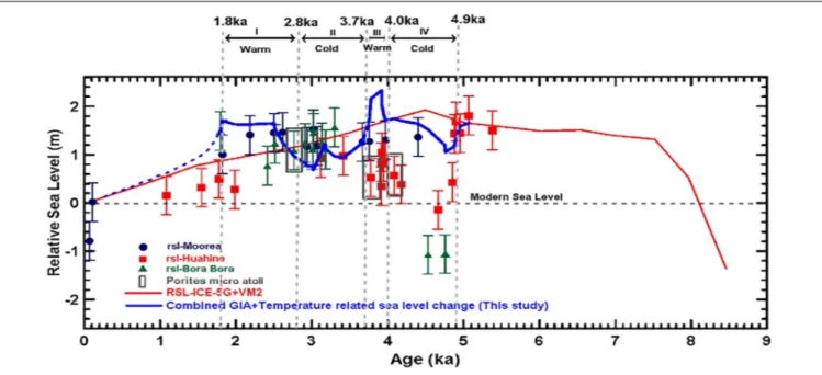
FIGURE 10 | Sea level-temperature relationships in the Pacific during the Holocene. Sea level estimates are from previously published study (Rashid et al., 2014) using empirical data and GIA model. Red curve represents the GIA model prediction of mean sea level curve for the Society Islands from Mid to Late Holocene. Individual data points represent sea level data obtained from coral samples from Moorea (blue), Huahine (red) and Bora Bora (green). The combined GIA-temperature relationship reveals the amplitudinal sea level variations, reconciling the discrepancy between the GIA estimation and the empirical observations between 2 to 2.6 ka.
between ∼2.8 and 3.8 ka and ∼4.1 and 4.9 ka were reported (Koutavas et al., 2002). Furthermore, our findings are in accord with high SSTs reported at ∼4 and 1.8 ka to 2.9 ka (Koutavas et al., 2002; Abram et al., 2009) in the Southern Pacific. This indicates that, first, the reported SST variability on the order of up to ± 2◦
C reflects the global temperature oscillations throughout the Mid to Late Holocene, and second, that solar activity seems to be the major driver of centennial to millennial scale SST changes throughout the Mid to Late Holocene, at least in the Southern Pacific.
Our proxy data also match the Holocene CO2concentration
curve reconstructed from Antarctic ice cores (Indermühle et al., 1999) (Figure 9D). The CO2 record of the last 6
ka indicates a distinct increase in CO2 concentrations of
about 16 ppm from about 264 ppm to about 280 ppm superimposed by second order variation in the range of a few ppm. This increase in CO2 may also be reflected in our SSTs.
However, the increase of about 2◦
C related to an increase of 16 ppm CO2 is too small compared to the amount of CO2
(∼100 ppm) assumed to change the temperature from pre-industrial to modern times by 0.8◦
C (IPCC, 2013). Probably, cyclic variations of the solar activity controlled the atmospheric temperature and SST variations in the Southern Pacific to a much larger extent.
Implications for the Sea Level and
Temperature Relationships in the Pacific
Our local to regional observations of periodic SST variations in the Pacific on the order of about 2◦C may have direct consequences for the height of the sea level on a larger
scale. Differentially regarded, first, viewed from a cause perspective the open and remote geologic and oceanographic setting implies that the record reflects rather global than a local cause. Thus, our records might be representative for SST changes in other regions too, potentially including a systematic time shift which may contribute to process identification. Second, from a consequence perspective, the related thermal expansion-driven sea level rise depends on the size of the affected water mass and could have direct impact on the adjacent coastlines. Recording such SST variation patterns in the far remote Pacific points to the involvement of large water masses, and therefore to the potential feedback mechanism to global currents and SST systematics. Alternating cool and warm SSTs cause water to expand or contract and the relative sea level to rise and fall. The general contribution from thermal expansion of the ocean has been quantified on global and multi-millennial time scales from 10,000 year integrations with six coupled climate models to be in the range from 0.20 to 0.63 m/◦
C (Levermann et al., 2013). In a recent study empirical sea level estimates were compared to Holocene sea level variations of numerical models taking only Glacial Isostatic Adjustments (GIA) related sea level variations into account, however, any SST-related variations have been neglected (Rashid et al., 2014). Although there is a general agreement between GIA modeled sea level variations and the empirical data, there are time intervals where empirical data indicate higher or lower sea level periods than those predicted from GIA modeling. This most likely illustrates that GIA is not the only factor controlling sea level, and rather cyclic SST
variations may superimpose GIA-controlled sea level height. In Figure 10 the GIA-related sea level fluctuations are combined with SST-caused amplitudinal variations taking a conservative SST-sea level relationship of about 0.2 m/◦
C into account. From Figure 10 (blue curve) it can be seen that the sea level corresponding to interval I (1.8 – 2.8 ka) and III (3.7 to 4 ka) is on average about 0.4 m higher than the GIA-controlled sea level alone. In contrast, for time intervals II (2.8 to 3.7 ka) and IV (4 to 4.9 ka) reconstructed sea level is lower than predicted from GIA modeling alone. For interval I the SST-GIA combined sea level curve fits the empirical data better than the theoretical GIA-related curve alone. Apart from interval III, for the intervals II and IV the combined SST-GIA sea level curve is in general agreement and within statistical uncertainties. However, this should be considered as first order interpretation with the question still remaining open to future improvements.
CONCLUSION
(1) Secondary inorganic aragonite precipitation in a coral sample could result in a shift in Sr/Ca, U/Ca, and δ18O towards higher values, and thus lead to cooler SST
estimates. Although our pre-screening routines revealed massive skeletal parts to be well-preserved, we speculate that even these parts may be affected by early diagenetic alterations, most likely due to percolation of seawater along interconnected micro-pores.
(2) The elemental contribution from secondary aragonite does not seem to be erratic, rather it appears to offset the values while still conserving original correlations among proxies. Thus, this may still allow the gathering of climatic information from affected samples by normalizing measured values relative to their mean values.
(3) The reconstructed relative SST variations (1SST) indicate centennial to millennial SST trends (intervals I to IV) on the order of ± 2◦
C even in corals affected by early diagenesis and despite the violation of ‘closed system behavior’. (4) Identified SSTs for intervals I to IV are in phase with
variations of the solar activity deduced from14C and10Be
variations measured in continental ice cores. This suggest that changes of solar activity likely played a major role in climate oscillations and sea level change throughout the Holocene in the Southern Pacific.
AUTHOR CONTRIBUTIONS
RR carried out sample preparation, analyses and data acquisition, and provided in his Ph.D. thesis the manuscript draft as a base for the submitted version, containing scientific contributions from all authors. AE obtained the coral samples, designed and directed the study and developed to a large extent the manuscript. VL supervised progress of the study, contributed to the scientific concept, and finalized the manuscript. JF, MW, SK, and HJ made significant scientific and analytical contributions bringing expertise on biomineralisation and various high-resolution and optical methods. FB, AR, and W-CD kindly provided expertise and scientific input on corals, paleo-SST systematics, and data interpretation. ES contributed scientific expertise and detailed knowledge on the sampling region and considered SST concepts. BL provided important scientific input on the initial concept of the study and early stage of the manuscript. All authors contributed to the article and approved the submitted manuscript version.
FUNDING
This study was supported through funds from ESF/CHECKREEF project (EI272/22-1 to AE; DU129/141-1 to W-CD; 20MA21-115944 and 200020-140618 to ES), by the collaborative research initiative CHARON (DFG Forschergruppe 1644 – Phase II) funded by the German Research Foundation, and by the GEOMAR Helmholtz Centre for Ocean Research Kiel. The Ph.D. program of RR was financially supported by the Tanzania Ministry of Education and Vocational Training (MoEVT) in collaboration with DAAD (Deutscher Akademischer Austauschdienst) fellowship. AR acknowledges support from Swiss National Science Foundation Project Number SNF 200021_149247.
ACKNOWLEDGMENTS
We gratefully acknowledge Ana Kolevica, Jutta Heinze, Patrick Reichert, Nicolaas Glock (from GEOMAR, Kiel) and Brendan Ledwig (Kiel University) for their assistance in sample processing and data analysis, and Ilona Schäpan (GFZ, Potsdam) for SEM imaging.
REFERENCES
Abram, N. J., McGregor, H. V., Gagan, M. K., Hantoro, W. S., and Suwargadi, B. W. (2009). Oscillations in the southern extent of the Indo-Pacific Warm Pool during the mid-Holocene.Quat. Sci. Rev. 28, 2794–2803.
AlKhatib, M., and Eisenhauer, A. (2017). Calcium and strontium isotope fractionation during precipitation from aqueous solutions as a function of temperature and reaction rate; II. Aragonite.Geochim. Cosmochim. Acta 209, 320–342.
Allison, N., Finch, A., Webster, J. M., and Clague, D. A. (2007). Palaeoenvironmental records from fossil corals: the effects of submarine
diagenesis on temperature and climate estimates.Geochim. Cosmochim. Acta 71, 4693–4703.
Allison, N., and Finch, A. A. (2004). High-resolution Sr/Ca records in modern Porities lobate corals: effects of skeletal extension rate and architecture. Geochem. Geophys. Geosyst. 5:Q05001.
Bard, E., and Frank, M. (2006). Climate change and solar variability: what’s new under the sun?Earth Planet. Sci. Lett. 248, 1–14.
Beck, J. W., Edwards, R. L., Ito, E., Taylor, F. W., Recy, J., Rougerie, F., et al. (1992). Sea-surface temperature from coral skeletal strontium/calcium ratios.Science 257, 644–647.