The Cryosphere, 14, 1105–1120, 2020 https://doi.org/10.5194/tc-14-1105-2020
© Author(s) 2020. This work is distributed under the Creative Commons Attribution 4.0 License.
Detailed detection of active layer freeze–thaw dynamics using
quasi-continuous electrical resistivity tomography
(Deception Island, Antarctica)
Mohammad Farzamian1,2, Gonçalo Vieira3, Fernando A. Monteiro Santos1, Borhan Yaghoobi Tabar4, Christian Hauck5, Maria Catarina Paz1,6, Ivo Bernardo1, Miguel Ramos7, and Miguel Angel de Pablo7
1Faculdade de Ciências, IDL, Universidade de Lisboa, Lisbon, Portugal 2Instituto Nacional de Investigação Agrária e Veterinária, Oeiras, Portugal
3Centre for Geographical Studies, IGOT, Universidade de Lisboa, Lisbon, Portugal
4School of Mining, Petroleum and Geophysics, Shahrood University of Technology, Shahrood, Iran 5Department of Geosciences, University of Fribourg, Fribourg, Switzerland
6CIQuiBio, Barreiro School of Technology, Polytechnic Institute of Setúbal, Lavradio, Portugal 7Universidad de Alcalá de Henares, Alcalá de Henares, Spain
Correspondence: Mohammad Farzamian ([email protected]) Received: 5 March 2019 – Discussion started: 20 May 2019
Revised: 10 January 2020 – Accepted: 24 January 2020 – Published: 25 March 2020
Abstract. Climate-induced warming of permafrost soils is a global phenomenon, with regional and site-specific vari-ations which are not fully understood. In this context, a 2-D automated electrical resistivity tomography (A-ERT) sys-tem was installed for the first time in Antarctica at Decep-tion Island, associated to the existing Crater Lake site of the Circumpolar Active Layer Monitoring – South Program (CALM-S) – site. This setup aims to (i) monitor subsurface freezing and thawing processes on a daily and seasonal basis and map the spatial and temporal variability in thaw depth and to (ii) study the impact of short-lived extreme meteoro-logical events on active layer dynamics. In addition, the feasi-bility of installing and running autonomous ERT monitoring stations in remote and extreme environments such as Antarc-tica was evaluated for the first time. Measurements were re-peated at 4 h intervals during a full year, enabling the detec-tion of seasonal trends and short-lived resistivity changes re-flecting individual meteorological events. The latter is impor-tant for distinguishing between (1) long-term climatic trends and (2) the impact of anomalous seasons on the ground ther-mal regime.
Our full-year dataset shows large and fast temporal resis-tivity changes during the seasonal active layer freezing and thawing and indicates that our system setup can resolve
spa-tiotemporal thaw depth variability along the experimental transect at very high temporal resolution. The largest resis-tivity changes took place during the freezing season in April, when low temperatures induce an abrupt phase change in the active layer in the absence of snow cover. The seasonal thaw-ing of the active layer is associated with a slower resistivity decrease during October due to the presence of snow cover and the corresponding zero-curtain effect. Detailed investiga-tion of the daily resistivity variainvestiga-tions reveals several periods with rapid and sharp resistivity changes of the near-surface layers due to the brief surficial refreezing of the active layer in summer or brief thawing of the active layer during win-ter as a consequence of short-lived meteorological extreme events. These results emphasize the significance of the con-tinuous A-ERT monitoring setup which enables detecting fast changes in the active layer during short-lived extreme meteorological events.
Based on this first complete year-round A-ERT monitor-ing dataset on Deception Island, we believe that this sys-tem shows high potential for autonomous applications in re-mote and harsh polar environments such as Antarctica. The monitoring system can be used with larger electrode spacing to investigate greater depths, providing adequate monitoring at sites and depths where boreholes are very costly and the
ecosystem is very sensitive to invasive techniques. Further applications may be the estimation of ice and water contents through petrophysical models or the calibration and valida-tion of heat transfer models between the active layer and per-mafrost.
1 Introduction
Although permafrost soils show currently a clear global warming trend due to climate change (Biskaborn et al., 2019), regional differences can be pronounced, which are not only due to regional climate differences but also due to het-erogeneous soil characteristics. One example is the Antarctic Peninsula (AP), where one of the strongest air temperature increases has been recorded since the 1950s. In spite of this general air temperature increase, the northwest of the Antarc-tic Peninsula showed a cooling trend between 1999 and 2015 (Turner et al., 2016; Oliva et al., 2016). Consequently, and contrary to the general trend, the seasonal surficial thaw layer of the ground above the permafrost (the active layer) de-creased, indicating that the climate signal is more complex than previously reported (Ramos et al., 2017).
The active layer of permafrost environments is not only a climate change indicator; its dynamic is also of extreme importance to terrestrial ecosystems, since it influences the hydrology, soil nutrient and contaminant fluxes, and geomor-phological processes, such as polar erosion and mass wast-ing. Furthermore, changes in active layer thickness may also affect infrastructure due to the effects it shows on the rhe-ological properties of the perennially frozen soil (Williams and Smith, 1989).
In moist polar environments, the transition zone between the active layer and the permafrost table is frequently char-acterized by the presence of a high content of interstitial ice, forming an ice-rich layer, some centimeters to decime-ter thick. This relates to the indecime-terannual variability in the active layer thickness. In warmer summers, the active layer thickens and water percolates downwards, concentrating at the permafrost table, refreezing at the beginning of the cold season. In cooler summers, the active layer is shallower and the previously formed ice does not melt. This ice-rich layer, still poorly characterized but with significance due to its im-pacts on soil behavior, is called the transient layer (Shur et al., 2005). A continuous monitoring of the physical properties of the active and transient layers is therefore essential for under-standing the permafrost dynamics and its potential impacts on climate feedbacks and local ecology.
Deception Island in the South Shetland archipelago, off northern Antarctic Peninsula, is an extraordinary natural lab-oratory for studying active layer and permafrost dynamics. The island is an active stratovolcano with widespread per-mafrost down to sea level except at spatially restricted locali-ties with geothermal anomalies, generally along faults
(Goy-anes et al., 2014). The soil surface is bare, with vegetation being almost completely absent, and permafrost is close to its climatic limit, since mean annual air temperatures are just below 0◦C (Bockheim et al., 2013; Ramos et al., 2017). The soil is composed by a mix of lavas, lapilli and pumice, which in some areas induce high thermal insulation, with a resulting active layer thickness of only 40 cm.
The shallow active layer and soil characteristics of De-ception Island, the easy access to the permafrost table, and the geographical setting in the maritime Antarctic and its geothermal characteristics have made the island one of the best-studied areas for permafrost research on the Antarctic Peninsula (e.g., Ramos et al., 2008, 2017; Vieira et al., 2010; Melo et al., 2012; Bockheim et al., 2013; Goyanes et al., 2014). Two permafrost and active layer monitoring sites within the Circumpolar Active Layer Monitoring – South Program (CALM-S) – and the Global Terrestrial Network for Permafrost (GTN-O/GCOS/IPA) including ground tem-perature boreholes and meteorological stations have been in-stalled at Irizar and Crater Lake.
So far, monitoring of the active layer dynamics in Antarc-tica was conducted using only 1-D borehole and meteorolog-ical data, which restricted the analysis to point information that often lacks representativeness at the field scale. In ad-dition, being an invasive technique, the drilling of boreholes disturbs the subsurface and is not feasible to conduct over large areas, especially in environmentally sensitive ecosys-tems such as the Antarctic. Also, the drilling of boreholes to monitor temperature in deeper layers is very expensive in Antarctica, which further limits the application of bore-holes for deep investigations and in areas with very hetero-geneous ground conditions. As a cost-effective and ecolog-ically non-hazardous alternative, 2-D geophysical monitor-ing, such as electrical resistivity tomography (ERT), allows for monitoring the spatiotemporal variability in the freezing and thawing characteristics of the active layer and the per-mafrost, as has been demonstrated in several applications in the European Alps (e.g., Hauck, 2002; Hilbich et al., 2008; 2011; Krautblatter et al., 2010; Ottowitz et al., 2011; Supper et al., 2014; Mewes et al., 2017; Mollaret et al., 2019). ERT is a non-invasive technique that is sensitive to the electrical con-ductivity (the reciprocal of electrical resistivity) of materials. Due to the large contrast between the resistivity of ice and water, the method has become popular in permafrost inves-tigation to distinguish between frozen and unfrozen soil and thus to monitor the active layer dynamics including freez-ing, thawfreez-ing, water infiltration and refreezing processes in a spatial context, which is sometimes very difficult to assess with only temperature boreholes. This technique is also being widely used to provide non-invasive estimates of spatiotem-poral unfrozen water content distribution due to the strong dependence of electrolytic conduction on the phase change of water to ice in earth materials (e.g., Hauck, 2002).
Although individual ERT measurements in Antarctica have been reported (e.g., McGinnis et al., 1973; Guglielmin
M. Farzamian et al.: Detailed detection of active layer freeze–thaw dynamics 1107
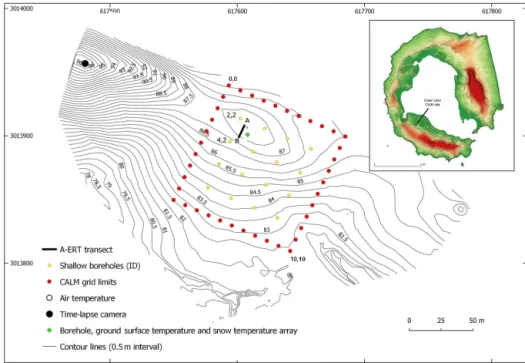
Figure 1. Location of Deception Island and Crater Lake CALM-S site in Antarctica.
et al., 1997; Gugliemin and Dramis, 1999; Hauck et al., 2007; Goyanes et al., 2014), no continuous and autonomous ERT monitoring has been attempted yet at these remote and ex-treme environments, where winter access is usually impossi-ble. In these cases, maintenance and repair, which have often become necessary in the autonomous ERT studies reported from the European Alps (cf. Supper et al., 2014), are not possible for most of the year. In this paper, we show that continuous ERT monitoring of the active layer and shallow permafrost is possible in Antarctica and that its results may yield high-resolution 2-D data on freeze and thaw character-istics on different timescales.
We installed and tested an autonomous and continuously measuring ERT monitoring system in the vicinity of shal-low boreholes at the Crater Lake CALM-S site, Deception Island, with the objective of evaluating its potential in a re-mote area without maintenance for a full year. The Crater Lake CALM-S site is typical for conditions found in Antarc-tica, where year-round stations are scarce, and most research stations are only operated in summer. Data were collected to monitor subsurface freezing and thawing processes on a daily and seasonal basis and to detect seasonal trends as well as the impact of short-lived extreme meteorological events. Short-lived meteorological events are rarely addressed in per-mafrost studies, but they reflect the impact of fast-changing meteorological conditions on the upper soil horizons. In the context of climate change, with increasing frequency of at-mospheric extreme events, these events may also become more frequent. Being able to identify them in the ERT se-ries allows for a better characterization of the links between soil thermal regimes and geomorphic dynamics.
2 Study area
Deception Island (62◦550S, 60◦370W) is located about 100 km north of the AP, in the Bransfield Strait, and is part of the South Shetland archipelago (Fig. 1). The island is a stra-tovolcano with a horseshoe shape and a diameter of 15 km, a 7 km wide caldera open to the sea, and maximum eleva-tion at Mount Pond (539 m). About 57 % of the island is currently glaciated and about 47 km2is glacier-free (Smellie and López- Martínez, 2002). The climate is cold oceanic, with frequent summer rainfall, a moderate annual tempera-ture range and mean annual air temperatempera-tures close to −3◦C at sea level. The weather conditions are dominated by the influence of the polar frontal systems, and atmospheric cir-culation is very variable, including the possibility for winter rainfall (Styszynska, 2004). Deception Island is an active vol-cano and is formed by intercalation of lava flows, pyroclastic and ash deposits, with many of the present-day glaciers being ash-covered. During the recent eruptions of 1967, 1969 and 1970, pyroclastic and ash deposits covered the snow man-tle, and buried snow is still present at some sites. Deposits are very porous and insulating, with high ice content at the permafrost table. The active layer is thin, varying from 30 to 96 cm depth across Deception Island in different soils (Bock-heim et al., 2013), and boreholes show the presence of warm permafrost.
The Crater Lake CALM-S site is located in a small and relatively flat plateau-like surface covered by volcanic and pyroclastic deposits at 85 m a.s.l., north of Crater Lake (62◦59006.700S, 60◦40044.800W). The site was selected due to
its flat characteristics, absent summer snow cover, large dis-tance to known geothermal anomalies, good exposure to the regional climate conditions (mitigating site-specific effects and being representative in a regional context) and vicinity to the Spanish station Gabriel de Castilla. The ground sur-face is completely devoid of vegetation, and the mean an-nual air temperature at the Crater Lake CALM-S site be-tween 28 January 2009 to 22 January 2014 was −3.0◦C. Per-mafrost temperatures are −0.3 to −0.9◦C, with permafrost thickness varying spatially from 2.5 to 5.0 m (Vieira et al., 2008; Ramos et al., 2017) and active layer thickness in the range of 25 to 40 cm. This spatial variability has not been addressed in the literature, but it is possibly related to differ-ences in surface deposits and snow cover.
3 Material and methods
3.1 Crater Lake CALM-S environmental monitoring setup
The Crater Lake CALM-S site consists of a 100 m ×100 m grid with little topography (maximum of 6 m variation in elevation) and was installed in January 2006 (Fig. 2), with several upgrades since then. The site includes monitoring of
Figure 2. Environmental monitoring setup at the Crater Lake CALM-S site.
air temperature, permafrost and the active layer in boreholes, and snow thickness. Thaw depth is measured manually once per year during summer at 121 nodes spaced at 10 m intervals by mechanical probing (Ramos et al., 2017).
Air temperatures are measured at 160 cm a.g.l. (above ground level), monitored with hourly measurements since 2009. Ground temperatures are measured in the shallow borehole S3,3down to 160 cm (node 3,3; Fig. 2). This
bore-hole has a diameter of 32 mm and is cased with air-filled PVC pipes, and ground temperatures are measured with iButton sensors at depths of 2.5, 5, 10, 20, 40, 80 and 160 cm. In ad-dition, ground temperatures are measured in 16 very shallow boreholes, regularly distributed within the grid, with a single iButton sensor close to the base of the active layer. Finally, snow thickness is estimated using a so-called snow pole, with iButton miniloggers installed on a vertical stake at 5, 10, 20, 40 and 80 cm height above the ground (de Pablo et al., 2016). Snow distribution is mapped using a Campbell CC640 time-lapse camera with daily pictures at 11:00, 12:00 and 13:00 (all times in local solar time). The combined approach of snow pole and the time-lapse camera allows evaluating the snow distribution in the study area.
3.2 Electrical resistivity tomography monitoring ERT is the method for the calculation of the subsurface elec-trical resistivity distribution from multiple elecelec-trical resis-tance measurements made using a quadrupole arrangement of electrodes. The electrodes are placed on the ground sur-face, and a 2-D or 3-D image of the resistivity distribution can be achieved by varying the location and spacing of the
electrodes. The relationship between the measured spatial apparent-resistivity distribution and the true resistivity distri-bution of the subsurface is complex and needs to be estimated using inversion theory (Loke, 2002). Under the assumption that general conditions (e.g., lithology, pore space) remain unchanged during the observation period, repeated resistivity measurement can provide a means for evaluation of freezing or thawing processes and subsurface temperature variations (Hauck, 2002).
An automatic ERT (A-ERT) monitoring system using a 4POINTLIGHT_10W (Lippmann) instrument was in-stalled in the vicinity of the ground temperature borehole S3,3
(see Fig. 2) in 2010 in order to monitor active layer freezing and thawing by ground surface time-lapse surveys (Fig. 3). The system was installed close to the interfluve, in the most elevated zone within the site, where stronger spatiotemporal subsurface variations are expected. The individual readings of each quadruple measurement were converted to apparent-resistivity values and stored in the internal memory.
All ERT surveys were performed using the Wenner elec-trode configuration to minimize energy consumption and measurement time as well as to obtain the best signal-to-noise ratio in highly resistive terrain (Kneisel, 2006; Hauck and Vonder Mühll, 2003). The Wenner array is also more sen-sitive to vertical changes in the subsurface resistivity below the center of the array (Loke, 2002), which makes the config-uration ideal for active layer imaging. Twenty copper plates, which are connected by buried cables to the active boxes, with an electrode spacing of 0.5 m were used in this study (Fig. 3b). A robust, waterproof box was used and buried, cas-ing the 4POINTLIGHT_10W instrument, solar-panel-driven
M. Farzamian et al.: Detailed detection of active layer freeze–thaw dynamics 1109
Figure 3. (a) Overview of the CALM-S site and (b) A-ERT monitoring system installation at CALM-S site. Electrodes are buried in the ground and are connected to the resistivity meter box by buried cables. (c) Resistivity meter box; the 4POINTLIGHT_10W instrument is connected to a solar-panel-driven battery and multi-electrode connectors . (d) A schematic display of the measured resistivity (pseudo-section) at the CALM-S site using a Wenner electrode configuration.
battery and multi-electrode connectors during data acquisi-tion (Fig. 3c). This setup yields 56 individual data points for each monitoring dataset at six data levels (Fig. 3d). A-ERT measurements were started at the beginning of 2010 and re-peated every 4 h during 1 full year.
3.3 A-ERT data processing and inversion
A-ERT data processing and inversion include several steps: data filtering (outlier detection), spatial mean apparent-resistivity analysis and apparent-resistivity data inversion. As a first step, the apparent-resistivity data measured during 1 year were filtered by removing data spikes and negative values. Furthermore, data points with standard deviations of more than 2 % after nine stackings were excluded. The quality of the apparent-resistivity data was good in most datasets, and less than 0.5 % of all measurements had to be eliminated. The measured apparent-resistivity data were then averaged for each depth level, providing six horizontal mean values for each dataset as shown in Fig. 3d and analyzed regarding daily and monthly resistivity changes.
In the next step, the apparent-resistivity datasets were inverted using the commercially available software RES2DINV. The robust inversion option in RES2DINV, as well as a mesh refinement to half of the electrode spacing, was applied to better resolve the expected strong resistivity contrasts between unfrozen and frozen subsurface materials. The objective function used in the robust inversion algorithm attempts to minimize the absolute changes in the resistivity
values which produce models with sharp interfaces between different regions with different resistivity values (Loke, 2002). In addition, a full 4-D inversion algorithm developed by Kim et al. (2009) was used to better image the temporal resistivity changes. The full 4-D inversion algorithm defines a subsurface structure and the entire monitoring data in the space–time domain to obtain a four-dimensional space–time model using just one inversion process. In this approach, regularization is introduced not only in the space domain but also in time, resulting in reduced inversion artifacts and improved stability of the inverse problem (Kim et al., 2009). 3.4 Virtual borehole analysis
A so-called virtual borehole analysis (e.g., Hilbich et al., 2011) was used to investigate the active layer dynamics dur-ing 2010 in more detail as well as to study the resistivity– temperature relationship. Here, inverted resistivity values were extracted from the tomogram along a 1-D depth tran-sect, close to the existing borehole S3,3. At this borehole,
temperature sensors are installed at different depths down to 160 cm, and temperature data are available every 3 h during the experiment. The maximum depth of the ERT investiga-tion is hereby almost equal to the deepest temperature sensor. The inverted temporal vertical resistivity variations from the tomogram are then compared to the corresponding temporal thermal variations obtained from S3,3.
Figure 4. (a) Snow thickness and air and soil surface temperature variability during the A-ERT data acquisition in 2010. (b) Borehole temperature plotted for the sensors installed at the node 3,3 (S3,3),
covering the investigation depth of the ERT transect. (c) Shallow borehole temperatures plotted for the sensors installed at nodes 2,2 and 4,2 at the base of the active layer. The dashed lines mark the selected dates for the ERT inversion analysis shown in Fig. 7.
4 Results and discussions
4.1 Analysis of observational data
Figure 4 shows air, surface, shallow and ground tempera-ture variations during the A-ERT monitoring period observed very close to the A-ERT transect. Snow cover during win-ter is thin, with only 10 to 20 cm thickness and frequent snow-free periods. Correspondingly, air and ground temper-ature are generally well-coupled, with a slight phase lag in the presence of snow (cf. the cooling events in August and September 2010).
The ground temperature at S3,3at shallow depths (Fig. 4b)
fluctuates significantly during the year, with temperatures ranging from −8 to 5◦C, reflecting the snow cover variability and air temperatures. Temperatures above zero are delineated by the yellow to red colors, indicating active layer thawing events. The temperature within the active layer falls below 0◦C at the end of April and stays below 0◦C until the
be-ginning of November. The zero-curtain phase in spring lasts around 1 month, whereas no significant zero curtain can be seen in autumn due to the low air and soil surface tempera-tures and the absence of a thick snow cover during freezing. Short-lived meteorological events with quick and superficial changes of the ground temperature around 0◦C are quite fre-quent during the study period, and therefore, brief surficial refreezing (e.g., in March, April and December) and thawing
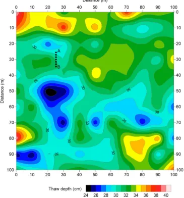
Figure 5. Spatial distribution of thaw depth measured at the grid nodes across the study area in January 2010. The location of the A-ERT transect is delineated with the black dotted line (A–B).
of the active layer (May) can be identified in the summer and winter respectively.
The temperature variations in the shallow temperature boreholes at nodes 2,2 and 4,2 (see Fig. 2 for the locations of the temperature sensors) are shown in Fig. 4c to investi-gate the lateral temperature changes along the A-ERT tran-sect. Node 2,2 is closer to the interfluve and is more exposed to the wind and sun. Consequently, thinner snow cover, as well as a smaller number of days with snow, was recorded at node 2,2 when compared to node 4,2, with corresponding lower winter temperatures at node 2,2 due to the stronger in-sulation effect of snow at node 4,2 (supported by time-lapse camera observations). The stability of temperatures at 0◦C in the summer months reflects the ice content and latent heat effects that limit thaw propagation.
Figure 5 shows the spatial distribution of thaw depth across the Crater Lake CALM-S site, measured in January 2010. The thaw depth varies between 25 to 40 cm, with shal-lower thaw depth in the south of the study area where the area is less wind-exposed, and shows a longer and more sta-ble snow cover. The thaw depth is approximately 30 cm along the A-ERT transect in January 2010.
4.2 Apparent-resistivity data
The apparent-resistivity raw data of all surveys were pro-cessed as discussed in Sect. 3.3, and the resulting mean daily apparent resistivity change of each data level is shown
M. Farzamian et al.: Detailed detection of active layer freeze–thaw dynamics 1111
Figure 6. (a) Mean apparent-resistivity data of the A-ERT profile during 2010 for different electrode spacing on a daily scale. (b, c) Mean apparent-resistivity data on the scale of individual events: (b) brief surficial refreezing event from 14 to 28 March 2010 and (c) brief surficial thawing event from 7 to 14 May 2010.
in Fig. 6a. The usefulness of investigating spatiotempo-ral apparent-resistivity data over different timescales was demonstrated in several studies (e.g., Hilbich et al., 2008, 2011). They allow insights into the resistivity variability trend during the year as well as the identification of the im-pact of specific meteorological events on the subsurface ther-mal regime. For most of the year, resistivity increase and decrease can be associated with freezing and thawing pro-cesses.
The apparent-resistivity data collected at a = 1 and 2 levels (corresponding to 0.5 and 1 m electrode spacing re-spectively) reveal a sharp resistivity rise on 19 April from approximately 10–20 k m and reaching values more than 500 k m on 5 May, suggesting the beginning of the sea-sonal freezing of the active layer. Because of the absence of snow cover during this period, the very low air temperature provokes an abrupt phase change, which causes a sharp re-sistivity rise in this period. The delayed response of deeper levels (i.e., a = 3, 4, 5 and 6, corresponding to 1.5, 2, 2.5 and 3 m electrode spacing respectively) indicates the advancing freezing front and is coincident with the gradual decrease in the active layer temperature with depth (see Fig. 4b). The freezing of the active layer intensifies in June, July and Au-gust. The beginning of the seasonal thawing phase is asso-ciated with the steady decrease in apparent resistivity, start-ing on 4 October from a value of approximately 200 k m to less than 40 k m at the end of October. During the sea-sonal thawing of the active layer, the snow cover dampens the thawing effect and provides water input to the active layer, which refreezes again at the still-frozen active layer. Inter-estingly, this zero-curtain phase, visible in the temperature
record, was reflected in the steady decrease in apparent resis-tivity, recorded by the A-ERT system in this period. Deeper levels experience the resistivity decrease with some delay.
In general, the daily apparent-resistivity fluctuations are relatively small. However, Fig. 6a reveals several significant resistivity fluctuations during the observation period. These fluctuations are associated with either brief surficial refreez-ing of near-surface layers in summer or short thawrefreez-ing pe-riods during winter as a consequence of short-lived meteo-rological extreme events with quick and superficial changes of the ground temperature around 0◦C. Two examples of these daily apparent resistivity changes during the short-lived events, events (I) and (II), were selected for detailed inves-tigation. Event (I), shown in Fig. 6b, is an example of the surficial refreezing of the active layer in the summer. A con-tinuous increase in apparent resistivity at shallower levels is evident with a total difference of approximately 30 k m in 10 d. On the other hand, event (II), shown in Fig. 6c, presents a very rapid apparent resistivity decrease at the shallowest levels, a = 1 and a = 2, with a total difference of approxi-mately 400–600 k m in 3 d. The observation of such rapid changes of the apparent resistivity proves the significance of the automatic ERT monitoring system to record continuous resistivity changes.
4.3 Monthly resistivity variations
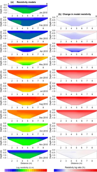
A monthly selection of the modeled resistivity data in 2010 and the resistivity changes relative to the first ERT dataset are shown in Fig. 7. Data collected on the 28th day of each month at 12:00 were used in this analysis, and all data were inverted
Figure 7. (a) Inverted resistivity tomograms of 12 monthly spaced A-ERT datasets between January and December 2010, based on data measured on the 28th of each month, and (b) relative resistivity changes based on the first ERT dataset referred to January.
using the full 4-D inversion algorithm, described in Sect. 3.3. The corresponding temperature profiles were marked with the dashed lines in Fig. 4b.
The resistivity pattern along the A-ERT monitoring tran-sect at CALM-S site is characterized by two vertical distinct resistivity zones. The first zone, down to 20–40 cm depth in summer, images the active layer. The resistivity of this layer changes dramatically during freezing and thawing. The deeper zone images the permafrost to a depth of 160 cm dur-ing the A-ERT measurements.
The resistivity model plotted for January shows a more conductive zone (less than 10 k m) for the first 30–40 cm,
followed by a deeper zone with resistivity of more than 30 k m. The shallow zone images the active layer in sum-mer, when this layer has not been frozen yet, and shows a slight thickness increase from the left to the right. The thickness and small lateral variability in this layer are in good agreement with the thaw depth measurement using a me-chanical probe in January 2010 (cf. Fig. 5). The resistivity and thickness of the active layer show a slight change during February and March. However, a more significant resistiv-ity decrease is evident at depths of more than 50 cm due to the slight temperature increase at depth during February and March (Fig. 4b), which increases the unfrozen water content and consequently decreases the subsurface resistivity.
The largest resistivity changes at the surface during the year take place between March and April due to the freez-ing of the active layer. Interestfreez-ingly, the resistivity of the permafrost at more than 1 m depth decreases slightly during this period. The resistivity model behavior in April can be well explained by an abrupt phase change during the active layer freezing in shallow surface and delayed response of the deeper zone. This is in very good agreement with the thermal transect shown in Fig. 4b, which shows a slight temperature increase at more than 1 m depth when compared to March. On the other hand, the resistivity model plotted for May is characterized by a resistivity decrease at the shallower zone (active layer) and a resistivity increase at depth (permafrost) when compared to the resistivity model for April. The resis-tivity increase in the permafrost is coincident with a temper-ature decrease in the permafrost during May, which results in lower unfrozen water content. On the other hand, the ac-tive layer warming during this month provides more unfrozen water to the active layer, which decreases the active layer re-sistivity during the same period.
The freezing of the active layer and cooling of permafrost intensifies during June, July and August, which is reflected by the high resistivity values. The beginning of seasonal thawing is then associated with the resistivity decrease in Oc-tober. The average resistivity of the active layer on 28 Octo-ber is higher than the corresponding zone during the thawing seasons (i.e., January, February, March, November and De-cember). This is due to the zero-curtain phase in October, when the snow cover damps the thawing effect and the tem-perature stays around zero. The steady resistivity decrease in the active layer and permafrost down to a depth of 160 cm is evident along the A-ERT transect during November and December due to the subsurface temperature increase. The monthly subsurface resistivity behavior is consistent with the mean apparent resistivity data shown in Fig. 6a.
4.4 Daily resistivity variations on the scales of individual events: events (I) and (II)
Two short-lived meteorological events with fast and superfi-cial changes of the ground temperature around 0◦C are se-lected for detailed A-ERT analysis to investigate how well
M. Farzamian et al.: Detailed detection of active layer freeze–thaw dynamics 1113
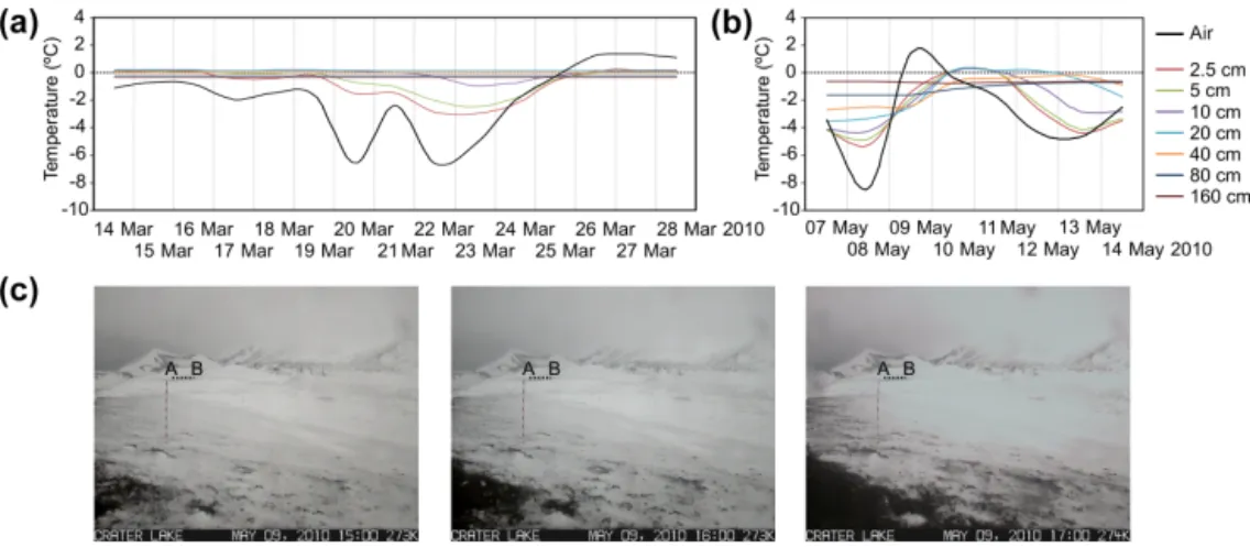
Figure 8. Air and ground temperature fluctuations on the event scale. (a) Event (I): brief surficial refreezing event from 14 to 28 March 2010. (b) Event (II): brief surficial thawing event from 7 to 14 May 2010. (c) Time-lapse camera photos at 11:00, 12:00 and 13:00 on 9 May.
the A-ERT model can resolve the expected sharp subsurface changes associated with the fast active layer freezing and thawing processes.
Figure 8a and b show in detail the air and ground tem-perature fluctuation during the selected events. Event (I) in-dicates a surficial refreezing of the active layer in the sum-mer. A decrease in air temperature started on 16 March and intensified on 20 March, with a subsequent increase start-ing on 22 March. The arrival of the cold air induced an impact in the uppermost 5 cm starting on 17 March, when the ground temperature at depths of 2.5 and 5 cm falls be-low zero. The active layer refreezing intensified between 22 and 24 March, when temperatures decreased and the advanc-ing freezadvanc-ing front reached 10 cm. A very shallow subsurface phase change is expected during this short-lived meteorolog-ical event, as no impact has been recorded at ground temper-ature sensors deeper than 10 cm.
Event (II) presents a surficial thawing of the active layer in summer. A drastic rise in the air temperature from −8.4 to 1.4◦C is evident on 9 May. The warm air influenced the
ground temperature immediately and generated an abrupt phase change in the top 20 cm on 10 May, as evidenced by the above-zero temperatures on 10 and 11 May at depths of 2.5, 5, 10 and 20 cm. The time-lapse camera photos taken on 9 May (Fig. 8c) show clearly the fast snowmelt between 11:00 and 13:00 on this day, which might explain the quick subsurface temperature rise due to the infiltration of the melted snow to the soil subsurface and consequent advective heat transfer. The thermal sensors at depths of 40 and 80 cm also recorded the temperature increase during this event, al-though temperatures stay below zero at these depths. Event (II) lasts for a shorter period compared to the event (I). How-ever, it caused stronger and deeper subsurface temperature changes.
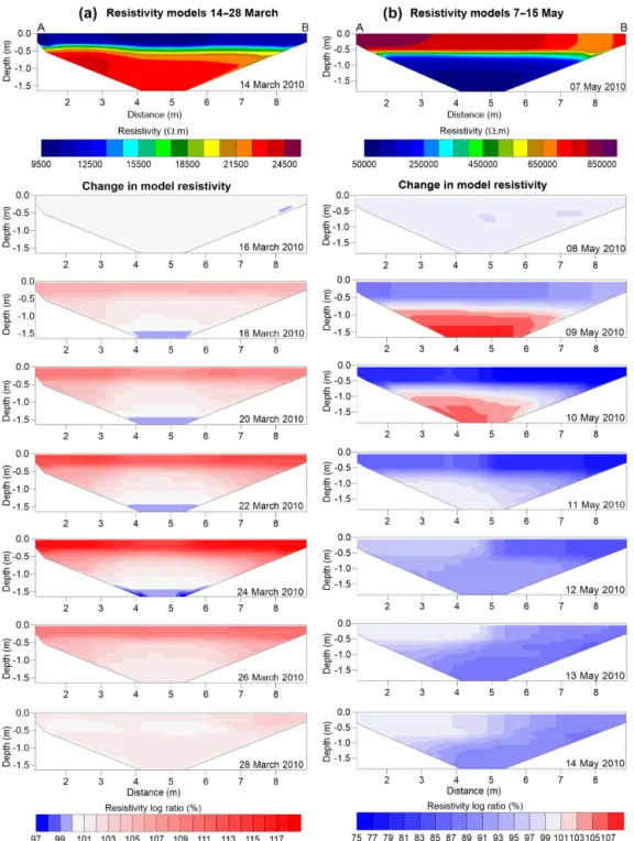
Figure 9 shows the time-lapse inversion results during events (I) and (II). Data collected on 14 March and 7 May were used as the reference for the events (I) and (II)
respec-tively, and the resistivity changes relative to the first ERT dataset are presented in this figure. Data collected at 12:00 were used in this analysis, and all data were inverted us-ing the full 4-D inversion algorithm, discussed in Sect. 3.3. A continuous resistivity increase at shallow depth (less than 30 cm) is evident from 18 to 24 March in Fig. 9a. The resis-tivity of this zone started to decrease again on 26 March, and there is no significant change between resistivity models on 28 March and the reference model on 14 March. In addition, no significant change occurs at depths of more than 30 cm during this event, suggesting that this event provoked phase changes only within the shallow subsurface. The results of the time-lapse resistivity models are in good agreement with the air and ground temperature fluctuation shown in Fig. 8a. The resistivity increase in the active layer is coincident with the temperature decrease in the active layer at shallow depth. The resistivity of the active layer reached its maximum be-tween 22 and 24 March, when the temperature reached its minimum and a larger amount of the pore water is frozen.
Figure 9b shows a sharp resistivity decrease on 9 May, suggesting an abrupt phase change during this day. In the following, the resistivity of the active layer reached its min-imum on 10 and 11 May. We anticipate that this is due to the infiltration of the snowmelt water into the soil subsur-face, which provides liquid water to the active layer and de-creases resistivity. A slight increase in resistivity at depths of more than 1 m is evident on 9 and 10 May. This can be explained by the slight permafrost temperature decrease at a depth of 160 cm on these days (cf. Fig. 8b). The contin-uous active layer refreezing during the following 3 d is co-incident with a slight resistivity decrease at depth. This can be explained with the delayed response of the permafrost to the temperature signal at the surface. An increase in the per-mafrost temperature at depths of 40 and 80 cm was recorded in the ground thermal sensors on these days.
Figure 9. Relative resistivity changes of daily spaced A-ERT datasets on the event scale. (a) Event (I): brief surficial refreezing event from 14 to 28 March 2010. (b) Event (II): brief surficial thawing event from 7 to 14 May 2010.
4.5 Temperature–resistivity relationship
The temperature–resistivity relationship for temperatures be-low zero was studied during two periods: (i) the beginning of the seasonal active layer freezing in April–May (P1) and (ii) the beginning of the seasonal thawing in October (P2). The selected A-ERT data were inverted using the full 4-D inversion algorithm, described in Sect. 3.3. The virtual
bore-hole analysis, described in Sect. 3.4, was used to establish the temperature–resistivity relationship.
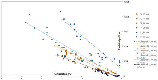
Figure 10 shows the linear regression between resistiv-ity and temperature in the virtual borehole at S3,3 for three
depths (i.e., 20, 40 and 80 cm). These depths were selected to study the resistivity–temperature behavior of the active layer (20 cm), permafrost table (40 cm) and permafrost (80 cm). The figure shows an excellent linear regression between re-sistivity and temperature at all depths during the seasonal
M. Farzamian et al.: Detailed detection of active layer freeze–thaw dynamics 1115 thawing (P2) in October with R2 greater than 0.96. Small
deviations from this linear relationship can be found during the seasonal freezing phase (P1) due to the faster subsur-face temperature and therefore phase change (no zero curtain present), where the mismatch between the volume measured by resistivity and temperature can be larger. In addition, the effect of downward ion migration upon freezing may further influence the relationship; however, a strong linear regres-sion between the resistivity and temperature at all depths can be also seen (R2greater than 0.86) for all depths during this period. The highest resistivity (and probably ice contents) is found at the 40 cm depth upon freezing, which may partly be due to more frequent refreezing effects at the boundary between the active layer and permafrost.
4.6 Evaluation of the temporal resistivity variability in the virtual borehole S3,3
Figure 11 shows the resistivity evolution with time in virtual boreholes at the S3,3 location during 2010 using the
eval-uation described in Sect. 3.4. As the RES2DINV software cannot invert more than 21 ERT datasets simultaneously, no time-lapse inversion algorithm was used for this analysis and apparent resistivity data were inverted independently using a batch routine. The 0◦C isotherm from the borehole temper-atures at S3,3(Fig. 4b) is superimposed on the resistivity
to-mogram. A resistivity cut-off value of 13 k m was selected to delineate the temporal variability in the thaw depth at the S3,3 location. This value was selected based on our analysis
of the individual resistivity tomograms as well as the average thaw depth measured by a mechanical probe in January. This value roughly corresponds to the resistivity transition value between the unfrozen media at the surface and the more re-sistive frozen zone at depth.
The average of thaw depth at the end of January is about 30 cm, with a slight increase in February. The brief active layer thinning between 20 and 24 February might have hap-pened due to the brief active layer cooling in this period, recorded by the ground temperature sensors. Afterwards, the thaw depth increases to an average of 40 cm at the begin-ning of March. The maximum thaw depth is recorded during March, probably due to the stronger active layer warming in this month. The sudden resistivity rise in the middle of March is coincident with the brief active layer freezing (event I), dis-cussed in Sect. 4.4. Thinning of the active layer starts in April due to the active layer cooling and possible refreezing of the infiltrating water above the permafrost table.
The largest resistivity changes in the active layer took place at the end of April due to the active layer freezing. The active layer stays frozen from May until October ex-cept during the brief surficial thawing event between 7 and 14 May (cf. Fig. 9b). The resistivity changes near the sur-face during the winter are coincident with consecutive active layer cooling and warming events. The resistivity values are greatest in winter and around the permafrost table at depths
around 40 cm. We anticipate that this is where maximal ice contents are present due to the repeated thawing and refreez-ing processes of water infiltratrefreez-ing from snow and rain that accumulated on top of the permafrost table (cf. the critical zone; Shur et al., 2005). During the zero-curtain phase in October–November, ground temperatures are still below zero and the active layer is still frozen. However, unfrozen mois-ture is already present due to snowmelt and the warm but subzero temperatures, which results in lower resistivity val-ues near the surface. The active layer thaws at the beginning of November, when the temperature rises above zero and is coincident with the strong resistivity decrease in this period. The average thaw depth in November–December is 20 cm, with a slight increase at the end of December. The sudden re-sistivity rise in December is coincident with the brief active layer freezing in this month.
5 Discussion
The monitoring setup with a very small electrode spacing (i.e., 50 cm) and dense measurements six times per day was designed to generate subsurface resistivity maps with very high spatial and temporal resolution. This enables detect-ing the expected fast and sharp resistivity changes within the very narrow active layer during the short-lived extreme me-teorological events at the study site. Since short-lived meteo-rological events may induce phase change, they are potential generators of geomorphic activity, such as cryoturbation, or even small debris-flows in sloping terrains. These events are particularly important in regions without a thick or contin-uous snow cover such as Deception Island due to the quick response of the active layer to the air temperature signal.
With this high-resolution setup, we were able to identify these events in our A-ERT models. Looking more closely at the resistivity and temperature changes during the brief active-layer thawing events, we suggest that infiltration pro-cesses from the melting snow cover are the dominating factor provoking the observed resistivity decrease and temperature increase. This is in agreement with Scherler et al. (2010), who simulated the active layer thaw period using a 1-D fully coupled heat and mass transfer model. They found that the water pool, formed at the ground surface from the melting snow cover, may percolate and reach greater depths, which results in fast water and advective heat transfer to depth. The infiltration ends when the water pool is emptied and/or the water refreezes. Such shallow active layer dynamics show that there are freeze–thaw cycles during the freezing season, which may result in cryoturbation and in sloping terrain, that are responsible for increased superficial solifluction.
The resistivity of both active layer and permafrost zones indicates only a slight lateral change along the transect, which is indicative for a spatially homogeneous ground con-ditions in the study area. However, the size of the A-ERT transect is comparatively small compared to other A-ERT
Figure 10. Resistivity values at the borehole location against borehole temperatures in S3,3during the seasonal active layer freezing in April
and May (P1) and thawing in October (P2).
Figure 11. Evaluation of the temporal resistivity variability in virtual borehole S3,3 inferred from inverted A-ERT data for the period
January 2010 to December 2010. The black line delineates the cut-off value of 13 k m, and the white dashed line shows the 0◦C isotherm from the borehole temperatures at S3,3.
studies where stronger lateral variations along the ERT tran-sects are usually more evident (i.e., Hilbich et al., 2011; Supper et al., 2014; Keuschnig et al., 2017). In contrast, large lateral resistivity changes are visible during the extreme short-lived meteorological events. An example of such lateral changes is very evident during event (II) shown in Fig. 9b. The obtained resistivity models during this event suggest the propagation of the thawing process from the left (A) to the right (B) on 9 and 10 May (i.e., the active layer resistivity decreased from the left to the right) and then refreezing from the same direction on 11 May. Because the left side of the A-ERT transect is closer to the interfluve and is more exposed to the wind and sun, subsurface thaw and snowmelt are ex-pected to take place from left to right along the transect ori-entation after the initial air temperature rise on 9 May. Sim-ilarly, active layer refreezing starts from the same direction (left to right) when the air cools down again on 11 May. On seasonal timescales, a similar lateral resistivity variation is visible in Fig. 7. During the freezing season, the resistivity of the active layer is higher on the left side due to the enhanced cooling of the active layer in this part of the profile. Similarly,
the resistivity of the active layer decreases from the left to the right during active layer warming (i.e., September 2010) and thawing (i.e., October 2010).
We used a resistivity cut-off value of 13 k m to distin-guish the unfrozen media at the surface (i.e., active layer) from the more resistive frozen zone (i.e., permafrost) at depth. This value was selected empirically based on our anal-ysis of the individual resistivity tomograms and the average thaw depth measured by a mechanical probe in January. The resistivity of the unfrozen media in the study area is compar-atively high compared to other studies conducted in alpine and polar regions (e.g., Supper et al., 2014; Keating et al., 2018) and could be due to the soil being composed by very porous lapilli, with high air content and large intergranular pore spaces that induce fast percolation of snowmelt and rainwater. The dark surface of the soil- and wind-exposed conditions promotes fast evaporation and favor quick drying of the near-surface horizons. In accordance with other stud-ies (e.g., Oldenborger and LeBlanc, 2018) the obtained linear relationship between resistivity and temperature also implies the absence of large latent heat effects during phase change,
M. Farzamian et al.: Detailed detection of active layer freeze–thaw dynamics 1117 i.e., comparatively dry conditions. In addition, in pyroclastic
sediments, pores containing water can be disconnected from each other, which further reduces the effect of phase change between liquid and frozen water on the bulk resistivity. It is worth mentioning that the resistivity of any subsurface mate-rial is a complex function of soil properties (e.g., grain and pore size, void ratio, degree of saturation, water content and salinity, temperature, and water phase), and thus the cut-off value cannot be used for other sites and a site-specific inves-tigation is required to estimate this value.
The detailed investigation of the resistivity tomograms in-dicates that our A-ERT setup could better map the thaw depth compared to the ground temperature sensor S3,3. In fact, the
thaw depth variability in the 10, 20 and 40 cm depth range, seen in the resistivity tomogram (Fig. 11), is not reflected in the borehole temperature data due to the lack of sensors between these depths. Hence, the ground temperature tomo-gram (Fig. 4b) shows a constant thaw depth of 40 cm in the first 3 months. These results reveal that our A-ERT setup al-lows for accurate characterization of the active layer freeze– thaw process, with a spatial resolution that can usually not be achieved with temperature sensors, except for a very dense sensor setup. In addition, the spatiotemporal resistivity vari-ations show that the resistivity values are greatest in win-ter and around the permafrost table at depths around 40 cm (see Fig. 11), indicating maximum ice contents at this depth. This is due to the repeated thawing and refreezing processes of water infiltrating from snow and rain that accumulated on top of the permafrost table (cf. the transition zone; Shur et al., 2005), which forms an ice-rich layer and increases the resistivity of this layer. Resistivity at the borehole location compared to borehole temperatures within S3,3(Fig. 10) also
shows remarkably greater values during active layer freezing at a depth of 40 cm, indicating that A-ERT data can be used to study the transition zone in the study area.
On the other hand, our resistivity models slightly overesti-mated the thaw depth during several periods, when compared to the borehole temperature data. Examples of such overesti-mations are seen in March, when inverted resistivity suggests the thaw depth to be slightly over 40 cm. This error becomes worse at the beginning of the seasonal thawing in November, when the A-ERT-derived thaw depth is too small (5 cm). We used a small electrode spacing of 50 cm to deal with the ex-pected abrupt changes close to the surface. However, the res-olution of the A-ERT within the first 10 cm (e.g., the active layer condition at the beginning of the seasonal thawing) is still very limited. In addition, the over-parameterized inverse problem and the effects of smoothing from regularization ap-plied in the inversion algorithm overestimate the thaw depth in the resistivity tomograms. In the virtual borehole analysis, each dataset was inverted independently, and temporal resis-tivity changes of individual quadrupoles were not accounted for in the inversion. Using a time-lapse inversion algorithm as used in Sect. 4.3 and 4.4 might enhance the temporal
reso-lution of the resistivity tomogram and reduce the uncertainty in the estimation of the thaw depth.
6 Conclusion and outlook
An automated ERT (A-ERT) system with a solar-panel-driven battery and multi-electrode configuration was in-stalled at Deception Island at the Crater Lake CALM-S mon-itoring site as the first automatic resistivity monmon-itoring sys-tem in Antarctica. Our analysis of this combined geophysical and thermal monitoring approach focused on (i) the ability of the A-ERT system to monitor the spatiotemporal variability in the active layer along the small-scale transect, (ii) the ac-tive layer freezing and thawing processes on seasonal time scales, and (iii) the impact of extreme short-lived meteoro-logical events on the ground thermal regime.
Based on the comprehensive analysis of the A-ERT data, the following main conclusions can be drawn:
1. The A-ERT system allows detailed monitoring of the spatiotemporal variability in the active layer in sum-mer. The maximum thaw depth in 2010 was recorded in March, with values slightly more than 40 cm. 2. The process of active layer freezing in autumn and
thawing in spring was well resolved by the A-ERT sys-tem. The absence of the snow cover and direct influence of atmospheric processes during the seasonal freezing provoked a drastic resistivity rise in April. On the con-trary, the zero-curtain phase during the seasonal thawing causes a continuous resistivity decrease during several weeks in November.
3. Short-lived meteorological events during a few days provoked a fast and dramatic resistivity change in the active layer due to the brief active layer freez-ing and thawfreez-ing, detected by the A-ERT system. Our study clearly shows that without automatic and quasi-continuous measurements, short-term active layer freez-ing and thawfreez-ing, and the infiltratfreez-ing water from the melting snow cover to the ground during such extreme meteorological events, could not be investigated. The automated system developed in this study allows a free choice of measurement interval as well as electrode configuration, and our A-ERT setup with a small electrode spacing of 0.5 m and dense measurements of six times per day enabled us to detect the impact of the extreme short-lived meteorological events on the active layer with a thick-ness as small as 20–40 cm. Interestingly, our A-ERT system could detect the spatial directions of the thawing and freez-ing processes along such a small transect. The A-ERT setup can also be applied with larger-spaced configurations to in-vestigate greater depths, enabling permafrost monitoring in Antarctica, where boreholes are very costly and the ecosys-tem is very sensitive to invasive techniques.
The consistency of our full-year results with previous stud-ies in more easily accessible alpine and polar regions (e.g., Hilbich et al., 2011; Supper et al., 2014; Keuschnig et al., 2017; Tomaskovicova, 2018; Oldenborger and LeBlanc, 2018) suggests that the detailed studies of the Alps can be transferred to setups in very remote environments, which would allow for integrative process studies as well as cou-pled modeling of A-ERT data with existing water content and temperature monitoring systems in Antarctica. Exam-ples of such studies include the combination of data pro-cessing techniques, petrophysical models and supporting in-formation to estimate unfrozen water content from electri-cal resistivity data (e.g., Hauck, 2002; Fortier et al., 2008; Grimm and Stillman, 2015; Dafflon et al., 2016) or combin-ing electrical resistivity data with seismic refraction data in a joint petrophysical model to estimate ice and water content (e.g., Hauck et al., 2011). Such analyses also provide a tool for monitoring the transient layer and studying the impact of fast-changing meteorological conditions and the frequent freeze–thaw process on soil behavior at the permafrost ta-ble. However, in the context of the volcanic material at De-ception Island, the link between pore water resistivity and measured bulk resistivity should be assessed by laboratory measurements prior to performing a quantitative investiga-tion on soil ice and water content. In addiinvestiga-tion, the type of the electric conduction needs to be investigated, as in dry soils with low salinity, surface conduction is the dominant process (Duvillard et al., 2018), as opposed to electrolytic conduc-tion, which is usually assumed to calculate water contents from resistivity values.
A long-term deployment of an A-ERT system in Antarc-tica would allow a much more detailed analysis of the per-mafrost and active layer evolution, which could be used as input data for hydrothermal models simulating the future per-mafrost evolution (e.g., Marmy et al., 2016; Rasmussen et al., 2018). In this context, joint A-ERT and thermal modeling ap-proaches such as the uncoupled modeling approach (Scherler et al., 2010) and fully coupled electro-thermal modeling ap-proach (Tomaskovicova, 2018) can be used for calibration of the thermal model that allows simulating heat transfer in ac-tive layer and permafrost. On a more local scale, the specific characteristics of Deception Island, where permafrost con-ditions are influenced also by geothermal and even volcanic activity, would allow for detailed investigations of the result-ing hydrothermal interactions in a cryospheric context. The fact that the monitoring occurs along a transect allows for im-proving the spatial understanding of the active layer dynam-ics with a minimal environmental disturbance in comparison to boreholes. It allowed detecting high-temporal resolution changes in freezing and thawing along the transect, provid-ing new insight also into the potential geomorphic dynamics and its regime, for example, for processes such as cryoturba-tion or solifluccryoturba-tion.
Data availability. The A-ERT and ground temperature data can be found at https://doi.org/10.5281/zenodo.3635063 (Farzamian et al., 2020). For inquiries please contact Mohammad Farzamian ([email protected]).
Author contributions. MF processed the A-ERT and borehole data, wrote the main part of the text, and generated the main results. GV contributed to the experimental design, installation and main-tenance of the A-ERT system; processing the borehole and snow cover data; and writing the text. FAMS designed the A-ERT survey and contributed to the elaboration of the methodology and writing of the text. BYT contributed to the processing of A-ERT data. CH contributed to the elaboration of the methodology, the discussion of the results, and the intermediate and final revision of the text. MCP contributed to the processing of the A-ERT data and the generation of the figures. IB built the A-ERT system and installed it at Decep-tion Island. MR, MAdP and GV installed the air, surface and ground temperature sensors; processed the temperature data; and measured the thaw depth at the site. All authors contributed to the revision of the paper.
Competing interests. The authors declare that they have no conflict of interest.
Acknowledgements. The research was funded by the Fundação para a Ciência e a Tecnologia under project PERMANTAR-2 (Per-mafrost and Climate Change in the Maritime Antarctic – FCT – PTDC/AAC-CLI/098885/2008) and the Portuguese Polar Pro-gram (PROPOLAR-FCT). We thank the Spanish Antarctic Station Gabriel de Castilla, the BIO Hespérides personnel for logistical support and the continued support of the Spanish Polar Commit-tee for the research on Deception Island. Gabriel Goyanes, Vanessa Baptista, José Miguel Cardoso, Ana David, Alice Ferreira and Mário Neves are thanked for the support in the maintenance of the A-ERT system. This work and publication have been supported by the FCT – project UIDB/50019/2020 – IDL, FCT – project UIDB/00295/2020 – and the Swiss National Science Foundation (project no. 178823). We are very grateful for the helpful and con-structive comments of the editor Christian Beer and two anonymous reviewers, who helped to significantly improve the paper.
Financial support. This research has been supported by the FCT (grant nos. UIDB/50019/2020 – IDL, FCT – project UIDB/00295/2020) and the Swiss National Science Foundation (project no. 178823).
Review statement. This paper was edited by Christian Beer and re-viewed by two anonymous referees.
M. Farzamian et al.: Detailed detection of active layer freeze–thaw dynamics 1119 References
Biskaborn, B. K., Smith, S. L., Noetzli, J. et al.: Permafrost is warm-ing at a global scale, Nat. Commun., 10, 264, 2019.
Bockheim, J., Vieira, G., Ramos, M., Lopez-Martinez, J., Ser-rano, E., Guglielmin, M., Wilhelm, K., and Nieuwendam, A.: Climate warming and permafrost dynamics in the Antarc-tic Peninsula region, Global Planet. Change, 100, 215–223, https://doi.org/10.1016/j.gloplacha.2012.10.018, 2013.
Dafflon, B., Hubbard, S., Ulrich, C., Peterson, J., Wu, Y., Wainwright, H., and Kneafsey, T. J.: Geophysical estimation of shallow permafrost distribution and properties in an ice-wedge polygon-dominated Arctic tundra region, Geophysics, 81, WA247–WA263, https://doi.org/10.1190/geo2015-0175.1, 2016. De Pablo, M. A., Ramos, M., Molina, A., Vieira, G., Hi-dalgo, M. A., Prieto, M., Jiménez, J. J., Fernández, S., Re-condo, C., Calleja, J. F., Peón, J. J., and Mora, C.: Frozen ground and snow cover monitoring in the South Shetland Is-lands, Antarctica: Instrumentation, effects on ground thermal be-haviour and future research, Cuad. Invest. Geográfica, 42, 475– 495, https://doi.org/10.18172/cig.2917, 2016.
Duvillard, P. A., Revil, A., Soueid Ahmed, A., Qi, Y., Coperey, A., and Ravanel, L.: Three dimensional electri-cal conductivity and induced polarization tomography of a rock glacier, J. Geophys. Res.-Solid Earth, 123, 9528–9554, https://doi.org/10.1029/2018JB015965, 2019.
Farzamian, M., Vieira, G., Monteiro Santos, F. A., Tabar, B. Y., Hauck, C., Paz, M. C., Bernando, I., Ramos, M., de Pablo, M. A.: A-ERT and ground tempera-ture data- 2010- Deception Island/Antarctica, Zenodo, https://doi.org/10.5281/zenodo.3635063, 2020.
Fortier, R., LeBlanc, A.-M., Allard, M., Buteau, S., and Calmels, F.: Internal structure and conditions of permafrost mounds at Umi-ujaq in Nunavik, Canada, inferred from field investigation and electrical resistivity tomography, Can. J. Earth Sci. , 45, 367– 387, https://doi.org/10.1139/E08-004, 2008.
Goyanes, G., Vieira, G., Caselli, A., Cardoso, M., Marmy, A., San-tos, F., Bernardo, I., and Hauck, C.: Local influences of geother-mal anogeother-malies on permafrost distribution in an active volcanic island (Deception Island, Antarctica), Geomorphology, 225, 57– 68, https://doi.org/10.1016/j.geomorph.2014.04.010, 2014. Grimm, R. E. and Stillman, D. E.: Field test of
detec-tion and characterizadetec-tion of subsurface ice using broadband spectral-induced polarisation, Permafrost Periglac., 26, 28–38, https://doi.org/10.1002/ppp.1833, 2015.
Guglielmin, M. and Dramis, F.: Permafrost as a climatic indicator in northern Victoria Land, Antarctica, Ann. Glaciol., 29, 131–135, https://doi.org/10.3189/172756499781821111, 1999.
Guglielmin, M., Biasini, A., and Smiraglia, C.: The contribution of geoelectrical investigations in the analysis of periglacial and glacial landforms in ice free areas of the Northern Foothills (Northern Victoria Land, Antarctica), Geogr. Ann. A, 79, 17–24, https://doi.org/10.1111/j.0435-3676.1997.00003.x, 1997. Hauck, C.: Frozen ground monitoring using DC
resis-tivity tomography, Geophys. Res. Lett., 29, 2016, https://doi.org/10.1029/2002GL014995, 2002.
Hauck, C. and Vonder Mühll, D.: Inversion and interpretation oftwo-dimensional geoelectrical measurements for detecting per-mafrost in mountainous regions, Perper-mafrost Periglac., 14, 305– 318. https://doi.org/10.1002/ppp.462, 2003.
Hauck, C., Vieira, G., Gruber, S., Blanco, J. J., and Ramos, M.: Geophysical identification of permafrost in Livingston Is-land, maritime Antarctica, J. Geophys. Res., 112, F02S19, https://doi.org/10.1029/2006JF000544, 2007.
Hauck, C., Böttcher, M., and Maurer, H.: A new model for estimating subsurface ice content based on combined elec-trical and seismic data sets, The Cryosphere, 5, 453–468, https://doi.org/10.5194/tc-5-453-2011, 2011.
Hilbich, C., Hauck, C., Hoelzle, M., Scherler, M., Schudel, L., Völksch, I., Vonder Mühll, D., and Mäusbacher, R.: Monitoring mountain permafrost evolution using electrical resistivity tomog-raphy: A 7-year study of seasonal, annual, and long-term varia-tions at Schilthorn, Swiss Alps, J. Geophys. Res., 113, F01S90, https://doi.org/10.1029/2007JF000799, 2008.
Hilbich, C., Fuss, C., and Hauck, C.: Automated Time-lapse ERT for Improved Process Analysis and Monitor-ing of Frozen Ground, Permafrost Periglac., 22, 306–319, https://doi.org/10.1002/ppp.732, 2011.
Keating, K., Binley, A., Bense, V., Van Dam, R. L., and Chris-tiansen, H. H.: Combined geophysical measurements provide evidence for unfrozen water in permafrost in the Advent-dalen valley in Svalbard, Geophys. Res. Lett., 45, 7606–761, https://doi.org/10.1029/2017GL076508, 2018.
Keuschnig, M., Krautblatter, M., Hartmeyer, I., Fuss, C., and Schrott, L.: Automated Electrical Resistivity Tomography Test-ing for Early WarnTest-ing in Unstable Permafrost Rock Walls Around Alpine Infrastructure, Permafrost Periglac., 28, 158– 171, https://doi.org/10.1002/ppp.1916 2017.
Kim, J. H., Yi M. J., Park, S. G., and Kim, J. G.: 4-D inver-sion of DC resistivity monitoring data acquired over a dynam-ically changing earth model, J. Appl. Geophys., 68, 522–532, https://doi.org/10.1016/j.jappgeo.2009.03.002, 2009.
Kneisel, C.: Assessment of subsurface lithology in mountain envi-ronments using 2D resistivity imaging, Geomorphology, 80, 32– 44, https://doi.org/10.1016/j.geomorph.2005.09.012, 2006. Krautblatter, M., Verlcysdonk, S., Flores-Orozco, A., and
Kemna A.: Temperature-calibrated imaging of seasonal changes in permafrost rock walls by quantitative electrical resistivity tomography (Zugspitze, German/Austrain Alps), Geophys. Res., 115, F02003, https://doi.org/10.1029/2008JF001209, 2010. Loke, M. H.: Tutorial: 2D and 3D Electrical Imaging Surveys,
Tech-nical Note, 2nd edn., Geotomo Software, Malaysia, 2002. Marmy, A., Rajczak, J., Delaloye, R., Hilbich, C., Hoelzle, M.,
Kot-larski, S., Lambiel, C., Noetzli, J., Phillips, M., Salzmann, N., Staub, B., and Hauck, C.: Semi-automated calibration method for modelling of mountain permafrost evolution in Switzerland, The Cryosphere, 10, 2693–2719, https://doi.org/10.5194/tc-10-2693-2016, 2016.
McGinnis, L. D., Nakao, K., and Clark, C. C.: Geophysical iden-tification of frozen and unfrozen ground, Antarctica, in: Pro-ceed. 2nd Internat. Conf. Permafrost, 13–28 July, Yakutsk, Rus-sia, 136–146, 1973.
Melo, R., Vieira, G., Caselli, A., and Ramos, M.: Suscep-tibility modelling of hummocky terrain distribution us-ing the information value method (Deception Island, Antarctic Peninsula), Geomorphology, 155–156, 88–95 https://doi.org/10.1016/j.geomorph.2011.12.027, 2012. Mewes, B., Hilbich, C., Delaloye, R., and Hauck, C.: Resolution
degra-dation induced by hydrological processes, The Cryosphere, 11, 2957–2974, https://doi.org/10.5194/tc-11-2957-2017, 2017. Mollaret, C., Hilbich, C., Pellet, C., Flores-Orozco, A.,
De-laloye, R., and Hauck, C.: Mountain permafrost degradation documented through a network of permanent electrical re-sistivity tomography sites, The Cryosphere, 13, 2557–2578, https://doi.org/10.5194/tc-13-2557-2019, 2019.
Oldenborger, G. A. and LeBlanc, A.-M.: Monitoring changes in unfrozen water content with electrical resistivity surveys in cold continuous permafrost, Geophys. J. Int., 215, 965–977, https://doi.org/10.1093/gji/ggy321, 2018.
Oliva, M., Nývlt, D., and Pereira, P.: Recent regional cli-mate cooling on the Antarctic Peninsula and associated im-pacts on the cryosphere, (December), STOTEN, 580, 210–223, https://doi.org/10.1016/j.scitotenv.2016.12.030, 2016.
Ottowitz, D., Jochum, B., Supper, R., Römer, A., Pfeiler, S., and Keuschnig, M.: Permafrost monitoring at Mölltaler Glacier and Magnetköp?, Berichte der Geologischen Bundesanstalt, 93, 57– 64, 2011.
Ramos, M., Vieira, G., Gruber, S., Blanco, J. J., Hauck, C., Hi-dalgo, M. A., Tome, D., Neves, M., and Trindade, A.: Permafrost and active layer monitoring in the Maritime Antarctic: Prelimi-nary results from CALM sites on Livingston and Deception Is-lands, US Geological Survey and the National Academies; USGS OF-2007–1047, Short Research Paper 070 https://pubs.usgs.gov/ of/2007/1047/srp/srp070/ (last access: 15 February 2019), 2008. Ramos, M., Vieira, G., De Pablo, M. A., Molina, A., Abramov, A., and Goyanes, G.: Recent shallowing of the thaw depth at Crater Lake, Deception Island, Antarctica (2006–2014), Catena, 149, 519–528, https://doi.org/10.1016/j.catena.2016.07.019, 2017. Rasmussen, L., Zhang, W., Hollesen, J., Cable, S.,
Chris-tiansen, H., Jansson, P. E., and Elberling, B.: Modelling present and future permafrost thermal regimes in North-east Greenland, Cold Reg. Sci. Technol., 146, 199–213, https://doi.org/10.1016/j.coldregions.2017.10.011, 2018. Scherler, M., Hauck, C., Hoelzle, M., Stähli, M., and Völksch, I.:
Meltwater infiltration into the frozen active layer at an alpine permafrost site, Permafrost Periglac., 21, 325–334, https://doi.org/10.1002/ppp.694, 2010.
Shur, Y., Hinkel, K. M., and Nelson, F. E.: The transient layer: implications for geocryology and climate change science, Per-mafrost Periglac., 16, 5–17, https://doi.org/10.1002/ppp.518, 2005.
Smellie, J. L. and López-Martínez, J.: Geological map of Decep-tion Island, in: Geology and Geomorphology of DecepDecep-tion Is-land, edited by: Smellie, J. L., López-Martínez, J., Serrano, E., and Rey, J., Sheet 6-A, 1:25.000, BAS GEOMAP Series, British Antarctic Survey, Cambridge, 2002.
Styszynska, A.: The origin of coreless winters in the South Shet-lands area (Antarctica), Pol. Polar Res., 25, 45–66, 2004. Supper, R., Ottowitz, D., Jochum, B., Romer, A., Pfeiler, S.,
Gru-ber, S., Keuschnig, M., and Ita, A.: Geoelectrical monitoring of frozen ground andpermafrost in alpine areas: field studies and considerations towards an improvedmeasuring technology, Near Surf. Geophys., 12, 93–115, https://doi.org/10.3997/1873-0604.2013057, 2014.
Tomaskovicova, S.: Coupled thermo-geophysical inversion for per-mafrost monitoring, PhD thesis, Department of Civil Engineer-ing, Technical University of Denmark, Technical University of Denmark, Department of Civil Engineering, 2018.
Turner, J., Lu, H.,White, I., King, J. C., Phillips, T., Hosk-ing, J. S., Bracegirdle, T. J., Marshall, G. J., Mulvaney, R., and Deb, P.: Absence of 21st century warming on Antarctic Penin-sula consistent with natural variability, Nature, 535, 411–415, https://doi.org/10.1038/nature18645, 2016.
Vieira, G., López-Martínez, J., Serrano, E., Ramos, M., Gruber, S., Hauck, C., and Blanco, J. J., Geomorphological observations of permafrost and ground-ice degradationon deception and Liv-ingston Islands, Maritime Antarctica, in: Proceedings of the 9th International Conference on Permafrost, edited by: Kane, D. and Hinkel, K., 29 June–3 July 2008, Fairbanks, Alaska, Extended Abstracts, Vol. 1, University of AlaskaPress, Fairbanks, 1839– 1844, https://doi.org/10.5167/uzh-3320, 2008.
Vieira, G., Bockheim, J., Guglielmin, M., Balks, M., Abramov, A. A., Boelhouwers, J., Cannone, N., Ganz-ert, L., Gilichinsky, D. A., Goryachkin, G., López-Martínez, J., Meiklejohn, J., Raffi, R., Ramos, M., Schaefer, C., Serrano, E., Simas, F., Sletten, R., and Wagner, D.: Thermal state of per-mafrost and active-layer monitoring in the Antarctic: advances during the International Polar Year 2007–2009, Permafrost Periglac., 21, 182–197, https://doi.org/10.1002/ppp.685, 2010. Williams, P. J. and Smith, M. W.: The Frozen Earth.
Fundamen-tals of Geocryology, Cambridge University Press, Cambridge, https://doi.org/10.1017/CBO9780511564437, 1989.