O
pen
A
rchive
T
oulouse
A
rchive
O
uverte (
OATAO
)
OATAO is an open access repository that collects the work of Toulouse researchers
and makes it freely available over the web where possible.
This is a publisher-deposited version published in:
http://oatao.univ-toulouse.fr/
Eprints ID: 3901
To link to this article: DOI:10.1109/TASL.2009.2038671
URL:
http://dx.doi.org/10.1109/TASL.2009.2038671
To cite this version: MIGNOT Rémi, HELIE Thomas, MATIGNON Denis. Digital
waveguide modeling for wind instruments: building a state-space representation based
on the Webster-Lokshin model. IEEE Transactions on Audio Speech and Language
Processing, 2010, vol. 18, n° 4, pp. 843-854.
ISSN 1558-7916
Any correspondence concerning this service should be sent to the repository administrator:
Digital Waveguide Modeling for Wind Instruments:
Building a State–Space Representation Based
on the Webster–Lokshin Model
Rémi Mignot, Thomas Hélie, and Denis Matignon
Abstract—This paper deals with digital waveguide modeling
of wind instruments. It presents the application of state–space representations for the refined acoustic model of Webster–Lokshin. This acoustic model describes the propagation of longitudinal waves in axisymmetric acoustic pipes with a varying cross-section, visco-thermal losses at the walls, and without assuming planar or spherical waves. Moreover, three types of discontinuities of the shape can be taken into account (radius, slope, and curvature). The purpose of this work is to build low-cost digital simulations in the time domain based on the Webster–Lokshin model. First, decomposing a resonator into independent elementary parts and isolating delay operators lead to a Kelly–Lochbaum network of input/output systems and delays. Second, for a systematic assem-bling of elements, their state–space representations are derived in discrete time. Then, standard tools of automatic control are used to reduce the complexity of digital simulations in the time domain. The method is applied to a real trombone, and results of simulations are presented and compared with measurements. This method seems to be a promising approach in term of mod-ularity, complexity of calculation, and accuracy, for any acoustic resonators based on tubes.
Index Terms—Acoustic signal processing, acoustic waveguides,
linear delay filters, partial differential equations, signal synthesis, state–space methods.
I. INTRODUCTION
S
TUDYING physical modeling for sound synthesis allows simulations of the behavior of musical instruments. Con-sequently, it leads to more realistic sounds, especially during attacks and note transitions, compared to signal processing ap-proaches. However, digital simulations in the time domain re-quire intensive computations from signal processors, and sim-plifications of the physical model have to be considered to make real-time simulations possible. Moreover, because of interac-tions between elements of an instrument, building a modular synthesizer proves difficult.Manuscript received April 02, 2009; revised November 09, 2009. Current ver-sion published April 14, 2010. This work was supported by the CONSONNES project, ANR-05-BLAN-0097-01 The associate editor coordinating the review of this manuscript and approving it for publication was Prof. Julius O Smith.
R. Mignot and T. Hélie are with IRCAM and CNRS, UMR 9912, 75004 Paris, France (e-mail: mignot@ircamfr; [email protected]).
D. Matignon is with the ISAE, Applied Mathematics Training Unit, Université de Toulouse, F-31055 Toulouse Cedex 4, France, (e-mail: [email protected]).
The purpose of the present work is to build a complete acoustic resonator by connecting several subsystems which mimic acoustic effects. Here, it is applied to a wind instrument: the trombone. The difficulty and the novelty is to include subtle phenomena to lead to a refined acoustic model, but with some care about the processor cost of simulations and the modularity of the model.
With the approach of digital waveguides (cf., e.g., [1]), some works have considered 1-D acoustic model of axisymmetric pipes based on the Webster horn equation (cf. [2]). Approx-imating a varying cross-section pipe by some cylinders or cones leads to the Kelly–Lochbaum scattering network (cf., e.g., [3]–[5]), which allows a low-cost digital simulation in the time domain. These models assume planar and spherical waves, respectively. For a more realistic behavior of the virtual instrument, in [6], [7], and [8], visco-thermal losses have been taken into account. This model of losses (cf. [9]) involves fractional derivatives, and is more accurate than more standard damping based on integer order derivative. In [10], a model of lossless flared pipes has been studied starting from the Webster equation, then in [11], considering the Webster–Lokshin model with visco-thermal losses (cf. [12]), the Kelly–Lochbaum net-work has been derived for lossy flared pipes with continuity of radius and slope ( -regularity of the shape). The latter models allow the approximation of the shape of flared pipe with a few pieces of pipe.
After modeling each element separately, it is necessary to put them together in order to build the whole resonator. In [13] and [14], the following modular method is proposed: deriving state–space representations of every element in discrete time, interconnection laws allow the calculation of the state–space representation of the whole resonator.
In a very recent work, an extended framework (based on [11] and the Webster–Lokshin equation) has been derived and allows the reconstruction of all models mentioned above ([3]–[11]). The novelty of the present work is the use of the formalism of [14], starting from the unifying model of the extension of [11]. Thanks to the modularity of the method, virtual wind in-struments can be easily built considering additional models: mouthpiece, sound radiation, tone-hole, lips, and reed for in-stance. Theoretical points are briefly presented and referenced; this paper focuses on the numerical method and some optimiza-tions for real-time simulation.
This document is organized as follows. Section II presents the problem statement and the formalism of the digital wave-guide networks, where all elements of an instrument are
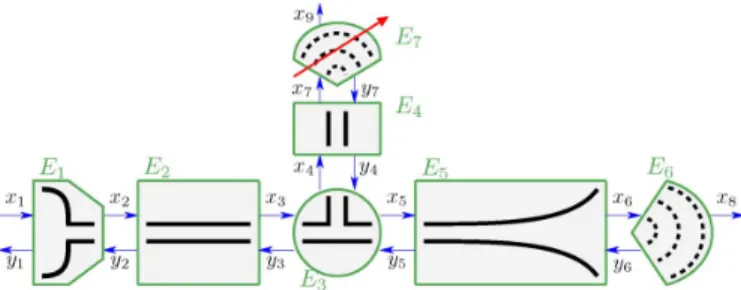
rep-Fig. 1. Example of an acoustic network modeling a resonator with a mouth-piece, a horn, and a tone-hole.
resented by input/output systems. In Section III, using given models, the analytical expressions of transfer functions of el-ements are derived. This section considers models of mouth-pieces, sound radiation, -port junctions and lossy flared pipes. The last one is characterized by the Webster–Lokshin equation. In Section IV, state–space representations are derived for all elements of Section III, in continuous time, then in discrete time. Section V presents standard tools of automatic control which allow the optimization of the numerical realization in order to obtain a low-cost digital simulation in the time do-main. Section VI presents the digital simulations of virtual trom-bones and the comparison between computed impedances and the measured impedance of a real trombone. The last section concludes this paper and deals with stability considerations and possible improvements of the optimization procedure.
II. PROBLEMSTATEMENT
A. Acoustic Waveguide Networks
Dynamic systems, which are described mathematically by sets of time-dependent Partial Differential Equations, can be modeled by networks of smaller input/output systems which ex-change signals. This approach appeared for modeling of elec-trical circuits in the 1970s with the Transmission Line Matrix approach (cf. [15]) and the Wave Digital Formulation (cf. [16]). In the 1980s appears the similar approach of the Digital Wave-guide Networks (cf. [17]) for acoustic systems. These methods of digital wave-based simulations are presented in [18] and [19]. Digital waveguide networks makes possible the representa-tion of a wind instrument by a network of elements which mimic acoustic effects of the pieces of the resonator. These elements are connected with respect to the topology of the real instrument, and exchange signals which are input and output variables.
The example of network in Fig. 1 models a possible res-onator with seven elements: element models the mouthpiece, elements , , represent air columns, element is a three-port junction connecting the three air columns, element represents the effect of the coupling with the sound radia-tion at the end of the horn, and element represents the sound radiation of a tone-hole. In this example, the sound radiation of the tone-hole has to be able to vary in order to take into account the action of a finger.
Examples of wind resonator construction using different models can be found in the literature. See, for instance [5], [20],
Fig. 2. Conversion two-portsC ,C ,C , andC .
and [21]. Moreover, this method allows a modular building and the simulation of imaginary instruments and it enables the exploration of new sounds with a physical validation.
B. Variables at Interfaces of Elements
At interfaces between two elements, the variables and are some acoustic states. A natural choice is to represent the acoustic states by the acoustic pressure and the particle flow (cf., e.g., [22]). Another choice, adapted to digital waveguide networks, consists of defining and using traveling waves which naturally satisfy the causality principle.
To have a common representation of acoustic states, a virtual reference pipe is introduced. It is a lossless cylinder with arbi-trary radius . Defined variables correspond to planar traveling waves for this reference pipe. With the speed of sound
m s , the mass density kg m and ; its characteristic impedance is , and planar traveling waves are
(1) In the case of lossy varying cross-section pipes, these vari-ables are neither decoupled nor perfectly progressive inside the pipe. Nevertheless, they remain “physically meaningful” at in-terfaces of pipe, and respect causality principle.
In order to make this change of variables with connections of input/output systems, conversion systems are recovered from (1). They are presented in Fig. 2.
This choice of variables is similar to that of [16], where the change of variables is defined with a resistance which can be arbitrary (where is the voltage and the current intensity).
C. Realizability and Delay Separation
Connecting discrete-time versions of each element (Fig. 1) involves delay-free loops so that it does not yield a realizable structure, as is, in the sense of automatic control theory. The implicit equations due to these delay-free loops can be solved using techniques such as Wave Digital Formulation (cf. [16]). In this paper, these equations are solved using standard alge-braic manipulations of state–space representations. This allows one the obtaining of a Kelly–Lochbaum framework which is op-timal in the sense that it reduces the number of transfer functions involved in the final digital waveguide network.
III. ACOUSTICMODELS OFRESONATORELEMENTS
This section presents the acoustic modeling of all elements which are used to build resonators of Section VI. First a refined model of varying cross-section pipes is studied, then possible models of the mouthpiece, sound radiation and -port junc-tions are presented. For each element, an -port system is de-rived with its transfer functions, for which inputs and outputs are variables .
A. Modeling a Piece of Pipe
1) Webster–Lokshin Model: The Webster–Lokshin model is a mono-dimensional model which characterizes linear waves propagation in axisymmetric pipes, assuming the quasi-sphericity of isobars near the inner wall (cf. [12]), and taking into account visco-thermal losses (cf. [9], [23], [24]) at the wall. The acoustic pressure and the acoustic particle flow are governed by the following equations, given in the Laplace domain:
(2) (3) where is the Laplace variable ( m is the angular frequency), is the space variable measuring the arclength of the wall, is the radius of the pipe, is the section area, quantifies the visco-thermal losses, and denotes the curvature of the wall. Equation (2) is called Webster- Lokshin equation, and (3) is Euler equation satisfied outside the visco-thermal boundary layer.
Note that the standard horn equation (cf. [2]) corresponds to (2) with no losses ( ) and assuming planar waves ( is replaced by the axis coordinate ). Straight and conical pipes are characterized by , and flared pipes are characterized by . In the following, is assumed to be non-negative, the negative case would require special treatments for deriving stable versions of digital waveguides (cf. [10]) which are out of the scope of this paper.
Denoting the radius of the pipe for the -ordinate, the arclength of the wall is , and
. In consequence, and when
.
For standard conditions, the physical constants are given by: the mass density kg m , the speed of sound
m s , the coefficient
m where and denote characteristic lengths of viscous ( ) and thermal ( ) effect (cf. [25]).
2) Two-Port System of a Piece of Pipe: In this paper, a pipe with varying cross-section is approximated by a concatenation of pieces of pipe with constant parameters. Thus, a piece of pipe is defined as a finite pipe with length , and with constant cur-vature and losses parameters (i.e and .
Notice that, except for a cylinder, and cannot be si-multaneously constant. In practice, pieces of pipe with constant curvature are considered, and is chosen as the mean of .
Fig. 3. Piece of pipe and its two-port systemQ .
This approximation makes sense, at least for realistic lengths and curvatures.
The piece of pipe is modeled by a system, where inputs are
and (incoming
waves at and ), and outputs are and (outgoing waves), this system is represented by the two-port of Fig. 3.
Solving (2) and (3) analytically together with (1), leads to the expressions of global transfer functions
(4) (5) (6) (7) with (8) and where denotes an analytical continuation of the positive square root of on a domain compatible with the one-sided
Laplace transform, namely (see
[26] and [27] for more details). The function is proved to be analytical in , and such that if . Functions and are rational functions of the variables
and .
Remark: Transfer functions and represent left (index l) and right (index r) global (index g) reflexions of the pipe (with length ) on traveling waves. “Global” means that every in-ternal effect of the pipe are mixed in these transfer functions. and represent global transmission of traveling waves through the pipe. An analysis of internal effects is detailed in next section.
3) Decomposed Framework: A detailed analysis of internal acoustic effects (cf. [11]) has enabled isolation of pure delay op-erators, which represent the traveling time of waves through the pipe. From this study, the Kelly–Lochbaum network has been recovered. Moreover, using the variable , a more detailed analysis has been done, and a new framework is derived. In this framework, which is proved to be equivalent to , the effects of geometry of the pipe are isolated from each other. The geo-metrical parameters are the radii at ends and , the slopes at ends and , the curvature and the visco-thermal losses of the
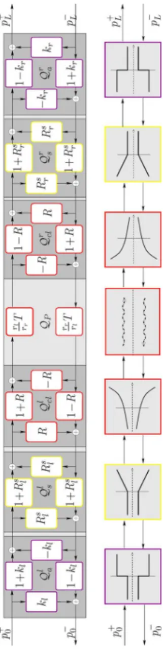
piece of pipe ( and ). The framework is presented in Fig. 4, and an interpretation of each cell follows.
• Cells and
and , with coefficients and , take into account sections of pipe and , at both ends. The index “a” means “area of section”. They are similar to cells of the framework of Kelly–Lochbaum after connection with a lossless cylinder of radius (cf., e.g., [3], [6]).
(9) (10) • Cells and
and , with transfer functions and , take into account slopes of pipe and
at left and right ends. The index “s” means “slope.” They are similar to cells of the framework of Kelly–Lochbaum after connection of cones (cf., e.g., [4], [7]).
(11)
with (12)
With some particular cases of junctions of cones (which correspond to or ), these transfer functions are unstable. This classic problem has been understood and solved in [7], [28]–[30] with some different methods. • Cells and
and , with the transfer function , take into account the constant curvature and losses of the pipe. The indexes “cl” means “curvature and losses”. With defined by (8)
(13) • Cell
This central cell represents the wave propagation with transfer function
(14) (15) In [26], is proved to be causal and stable with , so that represents the delay of wave propagation through the piece of pipe, and the effect due to the visco-thermal losses and the curvature.
The framework of Fig. 4 is interesting because the effects of the curvature and losses are isolated from the other (sections and slopes), and it makes their study easier. Because of the square roots of the function [cf. (8)], the study requires special treat-ments (see Section IV-A).
The six cells , , , , and of the framework of Fig. 4, can be rewritten as Fig. 5 shows. This simplification is used in [3], [4], and [11] to derive the Kelly–Lochbaum frame-work, in order to reduce the cost of calculation.
Fig. 4. Separation of the effects of pipe geometry.
Fig. 5. Simplification of cells.H(s) is any transfer function, and = 61.
B. Modeling the Mouth-Piece
The mouthpiece of a brass instrument is an element which is inserted at the beginning of the resonator, and where the player presses his lips. It is composed by an acoustic cavity (the cup) and a cone (the backbore). In [31], it is proposed to model the mouthpiece by an acoustic compliance for the cup, and a re-sistance and a mass for the backbore, , and , respectively (see Fig. 6). This modeling is a low frequency approximation1 but seems sufficient in respect of the small dimensions of the
1The mouthpiece is an important piece for the spectral envelope and the tone
color of the instrument. More accurate models can be found in [8], [19], but here we prefer to use a simpler model to present the formalism.
Fig. 6. Left: scheme of a mouthpiece. Right: equivalent electrical circuit.
Fig. 7. Two-port system for the mouthpiece.
mouthpiece. With kg m s the dynamic vis-cosity, the values of are given by
and (16)
From Fig. 6 the two-port system with is derived (see Fig. 7). and are given by
and (17)
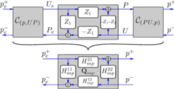
To obtain its equivalent two-port system with as inputs and outputs, two conversion two-ports are connected at each end (top of Fig. 7). The algebraic laws of interconnections (see Appendix I-A) lead to the two-port (see bottom of Fig. 7). The transfer functions of are given by
(18)
with
. C. Modeling Sound Radiation
At the output of the horn or at tone-holes, acoustic pressure and flow are linked by the radiation impedance . To sim-ulate this effect, the corresponding system is derived, for which left-end variables are and right-end output is the radiated pressure (right of Fig. 8). For any radiation impedance
, the radiation reflexion , and transmission are calculated using algebraic laws of interconnections (see Appendix I-A):
(19) (20)
Fig. 8. Equivalent system for the sound radiation.
Fig. 9. N-port junction.
Because of the flared end of the horn, the radiation model of a pulsating portion of a sphere (cf. [32]) seems appropriate for brass instruments. In this paper, this model is chosen for radiation at the end of the horn. Its impedance is denoted and its corresponding reflexion function . Their expressions are
(21)
(22)
with , and
where , and are optimized parameters of the approxi-mated model.
D. Modeling -Port Junctions
Junction elements are -port systems which allow the con-nection of elements, like pieces of pipe for instance (see Fig. 9). They are modeled with no spatial dimension, thus they have to satisfy pressure and flow continuity on all ports. By vention, positive flows go to the junction. Pressure and flow con-tinuities are equivalent to Kirchhoff’s laws for electrical circuits, and are written
for
Introducing [with (1)], and considering as known vari-ables and as unknown variables, solving this linear system leads to
(23)
where , and
. is the identity matrix, and is the matrix filled with 1 ( ).
Remark: Equation (23) is not new, but contrarily to some previous works, using variables , no impedance appears in
this equation. The only parameter is , which makes modular building easier.
IV. STATE–SPACEREPRESENTATION
For a systematic building of resonators, it is proposed to de-rive state–space representations for all elements. These repre-sentations allow algebraic manipulations on the system using well-known tools of automatic control (see Section V).
With the ( 1) vector of inputs and the ( 1) vector of outputs, each element is rewritten with the following repre-sentation in continuous time
(24) where is the ( 1) state vector, is the dynamics matrix,
is the control matrix, is the observation matrix, and is the direct link matrix. is the dimension of the system. Its discrete-time version is
(25) Pure delay operators are treated differently: for , if is commensurate with the sampling period ( with ), its discrete-time version is and is performed by a circular buffer. If is fractional, interpolation filters are needed (cf., e.g., [4], [33]).
In this section, state–space representations are derived in con-tinuous time for all elements presented in Section III, then using their diagonal forms, their discrete-time version are derived, but first, because the Webster–Lokshin model involves irrational transfer functions, it cannot be simulated so easily. It need to be approximated by finite-dimensional systems.
A. Finite-Dimensional Systems
Because of the square roots in , some involved transfer functions are irrational (cf. and of Section III-A4). These transfer functions have continuous lines of singularities in , which are named cuts. These cuts join some points (branching points) and the infinity. If , the function has one branching point at . The cut is chosen to preserve the hermitian symmetry. Therefore, transfer functions have a continuous line of singularities on . The residues theorem shows that these functions are represented by a class of infinite-dimensional systems, called Diffusive Representations (cf. [27], [34]–[36]). For any diffusive representation which is analytic on
(26) (27) For simulation in the time domain, in [35], it is proposed to approximate such diffusive representations by finite-dimensional approximations, given by where is the number of poles, is the position of the th pole and is its weight.
The poles are placed in with a logarithmic scale, and the weights are obtained by a least-square optimization in the Fourier domain.
If , has two more branching points, which are com-plex conjugate. In this case, the diffusive representations are ap-proximated with a finite sum of first and second order differen-tial systems
(28)
Transfer functions to approximate are: , and , for any (see Section III-A4). The order of approximation depends on the desired quality: mainly tunes the quality of approximation of effects due to visco-thermal losses, and , that due to the curvature. For example, in the case of large tubes, visco-thermal losses are negligible so that, the choice can be done. In practice, choosing and leads to fully satisfactory results, in most cases (which corresponds to a 16th-order filter). B. State–Space Representations in Continuous Time
In this section, the state–space representation of every ele-ment presented in Section III, is derived in continuous time.
1) -Port Junctions: These systems have no dynamics because they only contain constant coefficients. That leads to degenerate state–space representations where :
, , and
. However the state–space representation formalism stays convenient and most scientist calculation software manages empty matrices (Matlab©, Maple© for instance). From (23) the degenerate state–space representation of an -port junction is
(29) 2) Pieces of Pipe:
Cells and : These Cells only contain constant co-efficients and . With for example, the matrices of the degenerate state–space representation are
(30) Cells and : They contain one first-order transfer function, using the simplification of Fig. 5, the state–space rep-resentation of is
(31) Cells and : Using the approximation of diffu-sive representations (28), and the simplification of Fig. 5, the
state–space representation of is written with a diagonal form which follows:
(32) Cell : The central cell of the framework contains two pure delay operators which are simulated by circular buffers in discrete time, and two transfer functions for damping. These transfer functions are simulated by two approximation filters . Their state–space representation are
(33) 3) Mouthpiece: From the expression of the 4 transfer func-tions of the mouthpiece two-port [see (18)], the canonical form for the observation leads to the state–space representation which follows:
with and (34)
If , the matrix is diagonalizable in , then the change of variable is done where is the matrix of eigenvectors of . The diagonal matrix of dynamics is . The equivalent diagonal form is
(35) 4) Radiation: Using (22) and (20), the expression of the re-flexion and transmission radiation, the canonical form for the observation leads to the state–space representation which fol-lows:
with and (36)
If , the matrix is diagonalizable in , and its diagonalization is performed.
C. State–Space Representations in Discrete Time
The diagonal form of the previous state–space representations leads to independent one pole filters, which write
(37)
where and .
Then the use of discretization schemes yields discrete-time equations. Standard solutions are forward or backward Euler schemes, the bilinear transform, etc. In this paper, the so-called modified first-order hold (cf., e.g., [37]), that is, the exact dy-namics computed for a linearly interpolated input, is used. One nice property of the first-order hold is the ability to build the exact pole mapping.2 The corresponding difference equations are
for (38)
where
(39)
The matrix version is
(40) (41)
where for , and
.
Equation (40) is not a standard dynamics equation of state–space representation, because depends upon in the time domain. To cope with this problem, let us define the new state vector:
(42)
with , and .
To simplify notations, vectors and matrices of the discrete-time systems are denoted , , , , , , and .
V. REALIZABLENETWORK
This section is devoted to obtaining a computationally re-alizable network. First, from the previous network character-ized by the state–space representations of elements, delay-free loops are removed by concatenating elements without delay (cf.
2Note that, in the special case of convergent cones (cf. [30]), the first-order
hold has revealed to be more efficient than, e.g., the bilinear transform for the
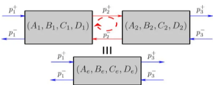
Fig. 10. Concatenating bi two-ports, with state–space representation.
Section V-A). Then, the complexity of the new network is re-duced using standard tools of automatic control consecutively (cf. Sections V-B–V-D).
A. Concatenating Elements
Because of an instantaneous loop, two connected elements without delay cannot be simulated in discrete time (see top of Fig. 10). To cope with this problem, it is possible to derive an equivalent two-port as the bottom of Fig. 10 shows.
In [33, pp. 31–33], the interconnection laws are performed from state–space representation and are given in Appendix I-B. This leads to the matrices , , and of the equivalent two-port.
This operation is performed recursively to remove every in-stantaneous loop, until the network only contains intertwined -port systems (without delay) and cells (with delay oper-ators).
B. Minimal Realization
At this stage of the building, a well-known result in automatic control allows the reduction of the dimensions of the systems, in order to reduce the cost of numerical computation.
For an original state–space representation, the study of its ob-servability allows knowledge of the existence of a state change, which defines observable and non-observable substates. From an input/output point of view it is not necessary to simulate the last substates, because they have no influence on the output.
Similarly, the study of reachability allows the separation of reachable and unreachable substates. With zero initial condi-tions, unreachable substates remain zero for bounded excita-tions .
Using the canonical form of Kalman (cf. [38]), the minimal realization is derived by eliminating non-observable or unreach-able substates. If they exist, the dimension of this minimal real-ization is lower than the original.
Remark: The Kelly–Lochbaum framework (Fig. 5 right part) corresponds to a minimal realization of the original cell (left part) in the sense of automatic control theory.
C. Jordan Decomposition
To reduce the cost of calculation, it is useful to look for a new change of state which makes the matrix sparse.
Considering the minimal realization of a system of the net-work, if its matrix is diagonalizable over , the modal form of the system is computed. If this matrix is not diagonal-izable, it always admits a Jordan decomposition over .
Then, the appropriate change of variable is done to lead to the new dynamics matrix with the diagonal form or the Jordan normal form. Such a matrix contains its complex eigenvalues on its diagonal, some 0 or 1 on its super-diagonal and 0 everywhere else.
D. Last Reduction
Whereas all systems are real-valued ( and ), matrices of the state–space representation are complex-valued. From a numerical point of view, computation with com-plex numbers is more expensive than with real numbers. How-ever, using the hermitian symmetry of input/output transfer ma-trix (that is ), it is possible to reduce the number of substates to calculate, as follows.
The matrix is with the Jordan normal form, then its Jordan blocks are sorted with respect to theixr eigenvalues. Real eigen-values appear first, complex eigeneigen-values with positive imagi-nary part appear second, and finally their complex conjugate ap-pear with the same order. This leads to the matrix
with is a Jordan matrix composed with real eigenvalues, is a Jordan matrix composed with complex eigenvalues with positive imaginary part, and .
Then can be decomposed as follows:
Using the hermitian symmetry of and by identifica-tions, the following properties are proved: and . Thus, the contribution of can be de-duced from that of .
Decomposing the state–space representation with
re-spect to eigenvalues of , ,
, and , the
equivalent scheme for simulation is, in the time domain
Moreover, using an appropriate change of variables, it is pos-sible to ensure that and are real matrices.
VI. RESULTS OFSIMULATIONS
A. Building Two Virtual Trombones
In this section, two virtual trombones are built with a mouth-piece, a varying cross-section pipe, and a radiation impedance. The target instrument is a Courtois trombone, for which the shape and the input impedance have been measured.
In the first case, the pipe is decomposed into 11 pieces of pipe, with some discontinuities of sections or slopes to have a refined fit with the measured shape. This model is denoted . The first piece is a cone at the junction between the mouthpiece and the pipe, the three following are cylinders for the slide, then two cones and two cylinders approximates the junction between the slide and the horn, and finally three flared pieces of pipe approximates the horn.
Fig. 11. Simulated system.
Fig. 12. Comparison (d) between the input impedance (a) measured on the real trombone and the computed impedances (b, forM ) and (c, for M ). The two latter curves are computed from the final discrete-time the state–space represen-tation of Section V and so they include approximations of type (28) and (38). Re-call thatM is built with 11 pieces of pipe, and M with only 5 pieces of pipe.
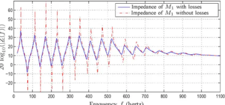
Fig. 13. Comparison of input impedances of M with and without visco-thermal losses. This comparison shows the effect of visco-thermal losses mainly in term of quality factor.
The second case is a simplification of the shape with only one cylinder and four flared pieces of pipe and with continuity of
section and slope at junctions. It leads to the Kelly–Lochbaum scattering network of [11], because of the -regularity of the radius.
Parameters of flared pieces of pipe, of and , have been chosen so that the shapes of the virtual pipes fit the real shape. Then, they have been adjusted by an optimization so that the computed impedance get closer to the measured impedance. The values of geometrical parameters used for the two models are given in Appendix II.
B. Simulated Systems and Computing Impedances
From the geometrical parameters of and , the respec-tive whole networks for simulations are built by following the procedures of Sections IV and V. These global systems which represent the resonator of a trombone, have one input and two outputs: the input is the incoming traveling wave at the entry of the mouthpiece, and their outputs are the traveling wave outgoing from the mouthpiece and the radiated pressure from the horn. In Fig. 11, and represent the global re-flexion and the global transmission, respectively.
Note that in the case of a complete sound synthesizer, and are used for the coupling between the exciter (lips for brass instruments) and the resonator, and is the output variable of the synthesizer.
The input impedance of a virtual trombone is computed, at the sampling frequency Hz, as follows.
• The impulse response of the global reflection is com-puted in the time domain. It is the response of for
with zero initial conditions, when . • Then is evaluated by a discrete
Fourier transform of .
• Finally, from (1), the normalized input impedance is (43) where denotes the section area at the entry of the resonator, which is the mouthpiece here.
C. Comparison of Impedances
In this section, the comparison between the measured input impedance and the impedances of and is presented. The measurements have been done with a Courtois trombone using the impedance sensor of the CTTM.3Impedances are presented in Fig. 12. The importance to take into account visco-thermal losses is illustrated in Fig. 13, where the impedance is calculated with and without losses
The main improvement of the model (with 11 pieces of pipes) compared to that of (with 5 pieces) concerns the spec-tral envelope. Whereas the envelope of maxima and minima of is smooth, that one of the measurements have some irreg-ularities (see the fifth and the sixth maxima for example). With a best fit with the real shape of pipe, the envelope of has the same type of irregularities. However, because of the simpli-fication of , the complexity of the network of simulation is reduced.
3Centre de Transfer de Technologie du Mans (CTTM), Le Mans, France.
VII. CONCLUSION ANDPERSPECTIVES
Using the formalism of state–space representations for digital waveguide networks leads to a good modularity for the assem-bling of elements, and an automatic building of the network of simulation. Moreover, standard tools of automatic control are used to reduce the cost of computation.
Considering the refined model of Webster–Lokshin for lossy flared pipes, it has been shown that this formalism can be applied with an approximation of the diffusive representations by finite-dimensional systems. Compared to models based on cylinders or cones, this model requires fewer pieces of pipe to obtain good geometrical fits and realistic computed impedances. This latter point is the main contribution of this work.
In this paper, only linear and static models have been pre-sented. In order to have a complete computer-aided maker of virtual wind instruments, nonlinear or time-varying system must be considered: trombone slide, valves, lips (cf., e.g., [39]), reed (cf., e.g., [5], [22]), tone-holes (cf., e.g., [5], [40]), brassy effect (cf., e.g., [41]). The modularity of the formalism should make an easy integration possible with few differences.
In Section VI, geometrical parameters of the model are chosen to fit the measured shape of pipe, then they are ad-justed by an optimization to lead to a realistic impedance. It seems interesting to go into details in this way. Moreover, the approximated impedance could be idealized, with a perfect harmonicity for instance.
In the case of -regular radius, the stability and the passivity of a network built by lossy flared pieces of pipe using the Web-ster–Lokshin model has been proved mathematically, but the ap-proximation of Section IV-A does not guarantee to preserve the stability and passivity of the whole network. At present these properties can only be checked a posteriori, before simulation. Nevertheless the automatic conservation of the stability and the passivity is under study.
Even if the order of simulated transfer functions is relatively high (16th order in most cases), the global complexity is com-pensated by the small number of simulated pieces of pipe. More-over, some extended methods of optimization may lead to a sig-nificantly reduced complexity. This promising point is under study.
APPENDIXI CONNECTINGTWO-PORTS
Connecting two systems consists in branching outputs of one system to inputs of the other. In Fig. 14, is defined as the equivalent two-port of the connection of and . In [14], the following notation is defined: , where is the equivalent relation and is the connection operator.
Merging these two-ports into a unique equivalent two-port is interesting for the following reasons.
• First, in some cases, merging allows the simplification of the framework.
• It can be used to prove the equivalence between some dif-ferent forms of a two-port system.
• As Fig. 14 shows, there is an instantaneous loop at inter-face, which cannot be simulated numerically as such. Here are presented two methods of concatenation.
Fig. 14. Connecting two-ports with transfer functions.
Fig. 15. Concatenating 2 two-ports, with state–space representations.
A) Algebraic Concatenation: The first algebraic method is performed from the transfer functions of two-ports and , and leads the analytical expressions of transfer functions of the equivalent two-port [see (44)–(47)]. These expressions are proved in continuous time and in discrete time. Studying stability of the transfer function of leads to study the roots of in the Laplace domain or in the -domain:
(44) (45) (46) (47) B) Concatenation With State–Space Representations: The second method is performed using the state–space representa-tions (cf. Fig. 15). With the block decomposition of and [see (48)], the discrete-time state–space representation of is performed in [33, pp. 31–33] and is given here by (49)–(52)
(48)
(49) (50) (51) (52)
where and are the inverse matrices of and , assuming they are invertible.
APPENDIXII
GEOMETRICALPARAMETERS OFMODELS
The following tables give the values of geometrical parame-ters used for the two trombone models of Section VI. The first model, , is the model with 11 pieces of pipe, and the second model, , is made with five pieces of pipe.
Mouthpiece parameters of and :
Pieces of pipe parameters of :
Pieces of pipe parameters of :
ACKNOWLEDGMENT
The authors would like to thank D. Ralley for proofreading, R. Caussé for giving data of the shape of the Courtois trombone, T. Hézard for measuring the input impedance of the trombone, and P.-D. Dekoninck for programming simulations and auto-matic builder of virtual wind instruments.
REFERENCES
[1] J. O. Smith, “Principles of digital waveguide models of musical in-struments,” in Applications of Digital Signal Processing to Audio and
Acoustics. Norwell, MA: Kluwer, 1998, pp. 417–466.
[2] A. Webster, “Acoustic impedance and the theory of horns and of the phonograph,” Proc. Nat. Acad. Sci. U.S, vol. 5, pp. 275–282, 1919.
[3] J. D. Markel and A. H. Gray, “On autocorrelation equations as applied to speech analysis,” IEEE Trans. and Electroacoust., vol. AE-21, no. 2, pp. 69–79, Apr. 1973.
[4] V. Välimäki, “Discrete-time modeling of acoustic tubes using frac-tional delay filters,” Ph.D. dissertation, Helsinski Univ. of Technol., Espoo, 1995.
[5] G. P. Scavone, “An acoustic analysis of single-reed woodwind instru-ments with an emphasis on design and performance issues and dig-ital waveguide modeling techniques,” Ph.D. dissertation, Music Dept., Stanford Univ., Stanford, CA, 1997.
[6] D. Matignon, “Représentations en variables d’état de guides d’ondes avec dérivation fractionnaire,” Ph.D. dissertation, Univ. Paris-Sud, Paris, France, 1994.
[7] E. Ducasse, “An alternative to the traveling-wave approach for use in two-port descriptions of acoustic bores,” J. Acoust. Soc. Amer., vol. 112, pp. 3031–3041, 2002.
[8] M. van Walstijn, “Discrete-time modelling of brass and reed woodwind instruments with application to musical sound synthesis,” Ph.D. disser-tation, Univ. of Edinburgh, Edinburgh, U.K., 2002.
[9] J.-D. Polack, “Time domain solution of Kirchhoff’s equation for sound propagation in viscothermal gases: A diffusion process,” J. Acoust., vol. 4, pp. 47–67, Feb. 1991.
[10] D. P. Berners, “Acoustics and signal processing techniques for phys-ical modeling of brass instruments,” Ph.D. dissertation, Stanford Univ., Stanford, CA, 1999.
[11] T. Hélie, R. Mignot, and D. Matignon, “Waveguide modeling of lossy flared acoustic pipes: Derivation of a Kelly–Lochbaum structure for real-time simulations,” in Proc. IEEE WASPAA, New Paltz, NY, 2007, pp. 267–270.
[12] T. Hélie, “Unidimensional models of acoustic propagation in axisym-metric waveguides,” J. Acoust. Soc. Amer., vol. 114, pp. 2633–2647, 2003.
[13] D. Matignon, “Physical modelling of musical instruments: Analysis/ synthesis by means of state space representations,” in Proc. Int. Symp.
Musical Acoust., Jul. 1995, pp. 496–502.
[14] P. Depalle and S. Tassart, “State space sound synthesis and a state space synthesiser builder,” in Proc. Int. Comput. Music Conf. (ICMC’95), Sep. 1995, pp. 88–95.
[15] P. J. Johns and R. L. Beurle, “Numerical solution of 2-dimensional scattering problems using a transmission-line matrix,” Proc. IEEE, vol. 118, no. 9, pp. 1203–1208, Sep. 1971.
[16] A. Fettweis, “Wave digital filters: Theory and practice,” Proc. IEEE, vol. 74, no. 2, pp. 270–327, Feb. 1986.
[17] J. O. Smith, “Music applications of digital waveguides,” Stanford Univ., Center for Comput. Res. in Music and Acoust. (CCRMA), Dept. of Music, 1987, Tech. Rep. STAN-M-39.
[18] S. Bilbao, Waves and Scattering Methods for Numerical Simulation. New York: Wiley, 2004.
[19] M. van Walstijn, “Wave-based simulation of wind instrument res-onators,” IEEE Signal Process. Mag., vol. 24, no. 2, pp. 21–31, Mar. 2007.
[20] M. van Walstijn and M. Campbel, “Discrete-time modelling of wood-wind instrument bores using wave variables,” J. Acoust. Soc. Amer., vol. 113, pp. 575–585, 2003.
[21] E. Ducasse, “Modélisation et simulation dans le domaine temporel d’instrumentsà ventà anche simple en situation de jeu: Méthodes et modèles,” Ph.D. dissertation, Univ. du Maine, Le Mans, France, 2001. [22] P. Guillemain, J. Kergomard, and T. Voinier, “Real-time synthesis of clarinet-like instruments using digital impedance models,” J. Acoust.
Soc. Amer., vol. 118, pp. 483–494, 2005.
[23] A. A. Lokshin and V. E. Rok, “Fundamental solutions of the wave equation with retarded time,” (in Russian) Dokl. Akad. Nauk SSSR, vol. 239, pp. 1305–1308, 1978.
[24] A. A. Lokshin, “Wave equation with singular retarded time,” (in Rus-sian) Dokl. Akad. Nauk SSSR, vol. 240, pp. 43–46, 1978.
[25] M. Bruneau, Manuel D’acoustique Fondamentale. Paris, France: Hermès, 1998.
[26] T. Hélie and D. Matignon, “Diffusive representations for the analysis and simulation of flared acoustic pipes with visco-thermal losses,”
Mathematical Models and Methods in Applied Sciences, vol. 16, pp.
503–536, Jan. 2006.
[27] D. Matignon, “Stability properties for generalized fractional differen-tial systems,” ESAIM: Proc., vol. 5, pp. 145–158, 1998.
[28] J. Martínez and J. Agulló, “Conical bores. Part I: Reflection functions associated with discontinuities,” J. Acoust. Soc. Amer., vol. 84, pp. 1613–1619, 1988.
[29] J. Gilbert, J. Kergomard, and J.-D. Polack, “On the reflection functions associated with discontinuities in conical bores,” J. Acoust. Soc. Amer., vol. 84, 1990.
[30] R. Mignot, T. Hélie, and D. Matignon, “Stable realization of a delay system modeling a convergent acoustic cone,” in Proc. Mediterranean
Conf. Control and Automat., Ajaccio, France, 2008, pp. 1574–1579.
[31] N. H. Fletcher and T. D. Rossing, Physics of Musical Instruments. New York: Springer-Verlag, 1991.
[32] T. Hélie and X. Rodet, “Radiation of a pulsating portion of a sphere: Application to horn radiation,” Acta Acustica, vol. 89, pp. 565–577, 2003.
[33] S. Tassart, “Modélisation, simulation et analyse des instrumentsà vent avec retards fractionnaires,” Ph.D. dissertation, Univ. Paris VI, Paris, France, 1999.
[34] O. J. Staffans, “Well-posedness and stabilizability of a viscoealistic in energy space,” Trans. Amer. Math. Soc., vol. 345, no. 2, pp. 527–575, 1994.
[35] G. Montseny, “Diffusive representation of pseudo-differential time-op-erators,” in ESAIM: Proc., 1998, vol. 5, pp. 159–175.
[36] T. Hélie and D. Matignon, “Representation with poles and cuts for the time-domain simulation of fractional systems and irrational transfer functions,” J. Signal Process., Special Iss. Fractional Calculus
Ap-plicat. in Signals and Syst., vol. 86, pp. 2516–2528, 2006.
[37] G. F. Franklin, J. D. Powell, and M. L. Workman, Digital Control of
Dynamic Systems. Reading, MA: Addison-Wesley, 1990, p. 151. [38] R. Kalman, “Canonical structure of linear dynamical systems,” Proc.
National Academy of Sci., pp. 596–600, 1961.
[39] C. Vergez, “Trompette et trompettiste: Un Système dynamique non linéaire analysé, modélisé et simulé dans un contexte musical,” Ph.D. dissertation, Univ. Paris 6, Paris, France, 2000.
[40] J.-P. Dalmont, C. J. Nederveen, S. Dubos, S. Ollivier, V. Meserette, and E. T. Sligte, “Experimental determination of the equivalent circuit of an open side hole : Linear and non linear behaviour,” Acta Acust., vol. 88, pp. 21–31, 2002.
[41] R. Msallam, S. Dequidt, R. Causse, and S. Tassart, “Physical model of the trombone including nonlinear effects. Application to the sound synthesis of loud tones,” Acta Acust., vol. 86, pp. 725–736, 2000.
Rémi Mignot received the Dipl. Ing. degree from
the Institut Galilée of University Paris XIII, Paris, France, in 2004, and the M.S. degree from the ATIAM of University Paris VI in 2006. He is currently pursuing the Ph.D. degree at Télécom ParisTech with the Laboratory Analysis/Synthesis Team at IRCAM-CNRS UMR 9912, Paris.
His research deals with physical modeling of wind instruments and numerical methods for digital simu-lation and sound synthesis.
Thomas Hélie received the Dipl. Ing. degree from the
Ecole Nationale Supérieure des Télécommunications de Bretagne, France, in 1997, and the Ph.D. degree in automatic and signal processing from the Université de Paris-Sud Orsay, France, in 2002.
After a postdoctoral research in the Laboratory of NonLinear System at the Swiss Federal Institute of Lausanne in 2003 and a lecturer position at the Uni-versité de Paris-Sud Orsay in 2004, he has been, since 2004, a Researcher at the National Research Council (CNRS) in the Analysis/Synthesis Team at IRCAM-CNRS UMR 9912, Paris, France. His research topics include physics of mu-sical instruments, phymu-sical modeling, nonlinear dynamical systems, and inver-sion processes.
Denis Matignon graduated from Ecole
Polytech-nique, Palaiseau, France, in 1990 and the Ph.D degree from the University Paris XI, Paris France.
In 1994, he was appointed Associate Professor in the Signal and Image Processing Department at Telecom Paris. He enjoyed a sabbatical stay with Sosso and Poems project teams at INRIA Rocquencourt in 2002–2003. In 2006, he obtained a Habilitationà Diriger des Recherches in Mathematics at University Paris VI. Since 2007, he has been a Full Professor and head of the Applied Mathematics training unit of Supaero syllabus at ISAE in Toulouse.
Prof. Matignon received the first prize for the best Ph.D. thesis in Automatic Control, a French national award given by AFCET for the years 1993–1994, for his Ph.D. thesis on “State–space representations of waveguide models with fractional derivatives” at the University Paris XI.