HAL Id: hal-01279599
https://hal.inria.fr/hal-01279599v2
Submitted on 22 Mar 2016
HAL is a multi-disciplinary open access
archive for the deposit and dissemination of
sci-entific research documents, whether they are
pub-lished or not. The documents may come from
teaching and research institutions in France or
L’archive ouverte pluridisciplinaire HAL, est
destinée au dépôt et à la diffusion de documents
scientifiques de niveau recherche, publiés ou non,
émanant des établissements d’enseignement et de
recherche français ou étrangers, des laboratoires
Transactional Memory
Naweiluo Zhou, Gwenaël Delaval, Bogdan Robu, Éric Rutten, Jean-François
Méhaut
To cite this version:
Naweiluo Zhou, Gwenaël Delaval, Bogdan Robu, Éric Rutten, Jean-François Méhaut. Autonomic
Par-allelism Adaptation on Software Transactional Memory. [Research Report] RR-8887, Univ. Grenoble
Alpes; INRIA Grenoble. 2016, pp.24. �hal-01279599v2�
ISSN 0249-6399 ISRN INRIA/RR--8887--FR+ENG
RESEARCH
REPORT
N° 8887
March 2016 Project-Team CompilerAdaptation on Software
Transactional Memory
Naweiluo Zhou, Gwenaël Delaval, Bogdan Robu,
Éric Rutten , Jean-François Méhaut
RESEARCH CENTRE GRENOBLE – RHÔNE-ALPES
Inovallée
Naweiluo Zhou123, Gwenaël Delaval12, Bogdan Robu45,
Éric Rutten 3, Jean-François Méhaut123
Project-Team Compiler Optimizations and Runtime Systems (CORSE) Research Report n° 8887 — March 2016 — 24 pages
Abstract: Parallel programs need to manage the time trade-off between synchronization and
computa-tion. A high parallelism may decrease computing time but meanwhile increase synchronization cost among threads. Software Transactional Memory (STM) has emerged as a promising technique, which bypasses locks, to address synchronization issues through transactions. A way to reduce conflicts is by adjusting the parallelism, as a suitable parallelism can maximize program performance. However, there is no universal rule to decide the best parallelism for a program from an offline view. Furthermore, an offline tuning is costly and error-prone. Hence, it becomes necessary to adopt a dynamical tuning-configuration strategy to better manage a STM system. Autonomic computing offers designers a framework of methods and tech-niques to build autonomic systems with well-mastered behaviours. Its key idea is to implement feedback control loops to design safe, efficient and predictable controllers, which enable monitoring and adjusting controlled systems dynamically while keeping overhead low. We propose to design feedback control loops to automate the choice of parallelism level at runtime and diminish program execution time.
Key-words: autonomic, transactional memory, feedback control, synchronization, parallelism adaptation
1Univ. Grenoble Alpes, LIG, F-38000, Grenoble, France 2CNRS, LIG, F-38000, Grenoble, France
3INRIA
4Univ. Grenoble Alpes, GiPSA-Lab, F-38000, Grenoble, France 5CNRS, GiPSA-Lab, F-38000, Grenoble, France
dans un système de mémoire transactionnelle logicielle
Résumé : L’exécution de programmes parallèles demande la gestion d’un compromis entre le temps de
synchronisation et le temps de calcul. Un haut degré de parallélisme peut diminuer le temps de calcul, mais augmenter le coût en temps de synchronisation entre processus légers. La mémoire transactionnelle logicielle (Software Transactional Memory, STM) est une technique prometteuse permettant de traiter le problème de synchronisation entre transactions en évitant les verrous. Une manière de réduire les conflits entre transactions est d’ajuster le degré de parallélisme, afin de trouver le niveau de parallélisme per-mettant de maximiser les performances du programme. Cependant, il n’existe pas de règle universelle permettant de décider du niveau de parallélisme optimal d’un programme hors ligne. De plus, un paramé-trage hors ligne est coûteux et peut entraîner des erreurs. Par conséquent, il est nécessaire d’adopter une stratégie de paramétrage et reconfiguration dynamique afin de mieux gérer un système STM. Le con-cept de calcul autonomique offre aux programmeurs un cadre de méthodes et techniques pour construire des systèmes autonomiques ayant un comportement maîtrisé. L’idée clé est d’implémenter des boucles de rétroaction afin de concevoir des contrôleurs sûrs, efficaces et prédictibles, permettant d’observer et d’ajuster de manière dynamique les systèmes contrôlés, tout en gardant bas le surcoût d’une telle méth-ode. Nous proposons de concevoir des boucles de rétroaction afin d’automatiser le choix du niveau de parallélisme à l’exécution, afin de diminuer le temps d’exécution du programme.
Mots-clés : système autonomique, mémoire transactionnelle, rétroaction, synchronisation, adaptation
1
Introduction
Multicore processors are ubiquitous, which enhance program performance through high parallelism (num-ber of simultaneous active threads). Although a high parallelism shortens execution time, it may also potentially increase synchronization time. Therefore, it is crucial to find the trade-off between synchro-nization and computation cost. The conventional way to address synchrosynchro-nization issues is via locks. However, locks are notorious for various issues, such as the likelihood of deadlock and the vulnerabil-ity to failure and faults. Also it is not straightforward to figure out the interaction among concurrent operations.
Transactional memory (TM) emerges as an alternative parallel programming technique, which ad-dresses synchronization issues through transactions. The accesses to the shared data are enclosed in transactions which are executed speculatively without blocking by locks. Various TM schemes have been developed [7, 6, 4] including Hardware Transactional Memory (HTM), Software Transactional Memory (STM) and Hybrid Transactional Memory (HyTM). In the report, we present the work on runtime pro-gram parallelism adaptation under STM systems where the synchronization time originates in transaction aborts. There are different ways to reduce aborts, such as the design of contention manager policy, the way to detect conflicts, the setting of version management and the choice of thread parallelism.
Online parallelism adaptation begins to receive attention recently. The choice of a suitable parallelism level in a program can significantly affect system performance. However it is onerous to set a suitable parallelism for a program offline especially for the one with online behaviour variation. When it comes to the program with online behaviour fluctuation, there is no single parallelism can enable its optimum performance. Therefore the natural solution would be to monitor the program at runtime and alter its parallelism when necessary.
We introduce autonomic computing [10] into STM systems to automatically regulate online program parallelism. In the report we argue that online adaptation is necessary and feasible for parallelism man-agement in STM systems. We demonstrate that the program performance is sensitive to the parallelism. We present two effective profiling frameworks for the parallelism adaptation on TinySTM [6].
2
Contribution
The main contributions of the report are as follows:
1. We propose two profiling frameworks which predict and apply the optimum parallelism at runtime. We develop a simple model to search and apply the optimum parallelism. We build an optimum parallelism predictor based on probability theory.
2. We dynamically resolve a CR range to detect the program phase change.
3. We utilise feedback control loops to regulate the parallelism. The control actions on parallelism are only taken when the contention of the program varies.
3
Background and Related Work
This section first reviews the background techniques and technologies for transactional memory (Sec-tion 3.1), then it gives a brief introduc(Sec-tion (Sec(Sec-tion 3.2) on autonomic computing. Lastly the related work and its comparison with our work are given.
3.1
Transactional Memory
Transactional memory (TM) is an alternative parallel programming technique. A transaction incorporates a set of read and/or write operations. Its accesses to the shared data are enclosed in transactions which are executed speculatively without blocking by locks. Each transaction makes a sequence of tentative changes to shared memory. When a transaction completes, it can either commit making the changes permanent to memory or abort discarding the previous changes made to memory [7]. Two parameters are often used in TM to indicate system performance, namely commit ratio and throughput. Commit ratio (CR) equals the number of commits divided by the number of commits and aborts; it measures the level of conflict or contention among the current transactions. Throughput is the number of commits in one unit of time; it directly indicates program performance. TM can be implemented in software, hardware or hybrid. Different designs explore the trade-off that impacts on performance, programmability and flexibility. In the report, we focus on STM systems and utilise TinySTM [6] as our experimental platform. TinySTM is a lightweight STM system which adopts a shared array of locks to control the concurrent accesses to memory and applies a shared counter as clock to manage the transaction conflicts.
The performance of STM systems has been continuously improved. The study to improve STM sys-tems mainly focus on the design of conflict detection, version management and conflict resolution. Con-flict detection decides when to check the read/write conCon-flict. Version management determines whether logging old data and writing new data to memory or vice versa. Conflict resolution, which is also known as contention management policy, handles the actions to be taken when a read/write conflict happens. The goal of the above designs is to reduce wasted work. The amount of wasted work resides in the num-ber of aborts and the size of aborts. The higher contention in a program, the larger amount of wasted work. The time spent in wasted work is the synchronization time in a STM view. Apart from dimin-ishing wasted work, one way to improve STM system performance is to trim computing time. A high parallelism may accelerate computation but resulting in high contention thus high synchronization time. Hence parallelism can significantly affect a program performance.
3.2
Autonomic Computing
Autonomic computing [9] is a concept that brings together many fields of computing with the purpose of creating computing systems that self-manage. A system is regarded as an autonomic system if it supports one of the following features [10]: (1) self-optimization, the system seeks to improve its performance and efficiency on its own; (2) self-configuration, when a new component is introduced into a system, the component is able to learn the system configurations. (3) self-healing, a system is able to recover from failures; (4) self-protection, a system can defend against attacks.
In the report, we concentrate on the first feature: self-optimization. We introduce feedback control loops to achieve autonomic computing. A classic feedback control loop is illustrated in Figure 1 in the shape of a MAPEK loop proposed by IBM.
In general, a feedback control loop is composed of (1) autonomic manager, (2) sensor (collect infor-mation), (3) effector (carry out changes), (4) managed element (any software or hardware resource). An autonomic manager (also seen as a controller) is composed of five elements:
1. monitor: this is used for sampling.
2. analyser: analysing date obtained from the monitor. 3. knowledge: knowledge of the system.
4. plan: utilise the knowledge of the system to carry out computation. 5. execute perform changes.
Managed Element
sensor Effectors
Monitors Knowledge Execute Autonomic Element
Analyse Plan
Autonomic Manager
Figure 1: A MAPEK control loop. It incorporates an autonomic manager, a sensor, an effector and a managed element among which the autonomic manager plays the main role.
3.3
Related Work
It has been been addressed in a few previous work [1, 2, 13, 5, 11] to dynamically adapt parallelism via control techniques to reduce wasted work in TM systems. Ansari et.al.[1, 2] proposed to adapt the parallelism online by detecting the changes of the application’s CR. The regulation action is made to the parallelism if the CR falls out of the pre-set CR range or is not equal to a single fixed CR value. This is based on the fact that CR falls during phases with high contention and rises when low contention. Ansari
et.al.gave five different algorithms which decide the profile length and the level of parallelism.
Ravichan-dran et.al.[11] presented a model which adapts the thread number in two phases: exponential and linear
with a feedback control loop. Rughetti et.al. [13] utilise a neural network to enable the performance prediction of STM applications. The neural network is trained to predict the wasted transaction execution time which in turn is utilised by a control algorithm to regulate the parallelism. Didona et.al. [5] intro-duces an approach to dynamically predict the parallelism based on the workload (duration and relative frequency, of read-only and update transactions, abort rate, average number of writes per transaction) and throughput, through one feedback control loop its prediction can be continuously corrected.
Our approaches differ from the previous work as (1)comparing with Ansari et.al., we resolve a CR range which is adaptive to the online program behaviour rather than a fixed range or value; (2)comparing with the parallelism prediction by Didona et.al., Ravichandran et.al. and Rughetti et.al., we present a model which predicts the optimum parallelism based on probabilistic theory which requires no offline training procedure or to try different thread number to search the optimum; (3)comparing with the afore-mentioned work which either only use CR or throughput to indicate the performance, we employ both: CR to indicate the program phase and throughout to indicate the correctness of the parallelism regulation.
4
Control of Autonomic Parallelism Adaptation
In this section, we detail the design of the feedback control loop for parallelism adaptation. We present two models which yield optimum parallelism at runtime. We firstly introduce a simple model which searches the optimum parallelism, then we present a more sophisticated model probabilistic model based on probability theory which directly predicts the optimum parallelism.
1st profiling
non- ac�on interval (�med by Tx)
...
Parallelism profile interval
Program starts A parallelism profile starts
decision point decision point
one profile length ...
...
one profile length
decision point
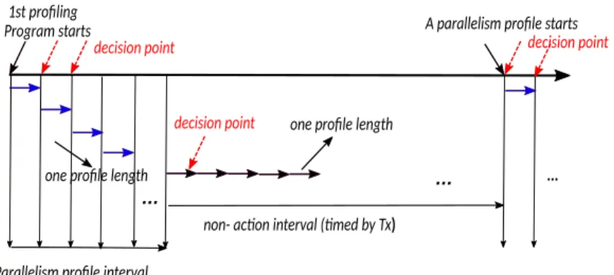
Figure 2: Periodical profiling procedure. The actions are taken at each decision point (marked by dashed red arrow). A profile length is a fixed period for information gathering, such as commits, aborts and time.
We measure three parameters from the STM system, namely the number of commits, the number of aborts and physical time. The number of commits and the number of aborts are addressed as commits and aborts in the rest of the report. We choose CR and throughput as the indicators to denote program performance, as CR and throughput are both sensitive to thread variation. But only one of them is not sufficient enough to represent the program performance, as:
• A high throughput shows fast program execution whereas a low throughput represents slow pro-gram progress. But a low throughput may be caused by a low parallelism or simply just a few transactions are due to execute at certain phase.
• CR indicates the conflicts among threads. A high CR means low synchronization time whereas a low CR mean high synchronization time. But a low CR can bring a high throughput when a large number of transactions are executing concurrently, whereas a high CR may give low throughput due to a small number of transactions executing concurrently.
The controller observes CR to detect the contention fluctuation and enable the corresponding control actions. The correctness of the control actions are verified by checking if the throughput is improved after the taken actions.
4.1
Overview of the Profiling Algorithm
To achieve autonomic thread adaptation which enables a program to always work under its optimum parallelism, we propose to periodically profile the applications at runtime. By observing CR, we can obtain the contention information of an application. However CR fluctuates in a certain CR range at the same program phase where the contention is relatively stable. When a program enters a new phase, the current parallelism will produce a different CR which falls out of the current CR range. This CR range fluctuation will trigger a new thread control action. Initially the two CR thresholds (CR_UP, CR_LOW) are both set to be 0 and are trained in the later profile stage. When the CR falls out of the thresholds, a new parallelism may be required to control the conflicts of the program in order to obtain the optimum throughout. The detail of the profiling procedure is illustrated in Figure 2.
The parallelism profiling procedure starts once the program starts. Initially the program creates a pool of threads, among which only 2 threads are awaken and the rest are suspended. At each decision point, which corresponds to one state of the automaton in Figure 3(b), the control loop (see section 4.2) is activated to regulate the parallelism or suspend the parallelism regulation. A profile length is a fixed period for information gathering, such as commits, aborts and time. A parallelism profile interval is
composed of a continuous sequence of profile lengths within which the parallelism is adjusted and the CR range is computed. The non-action interval is composed of one or a continuous sequence of profile lengths, within which the parallelism regulation is suspended. The duration of parallelism profile interval and non-action interval are not fixed values as we can see from Figure 2. The above procedure continues until the program terminates.
4.2
Feedback Control Loop of the Simple Model
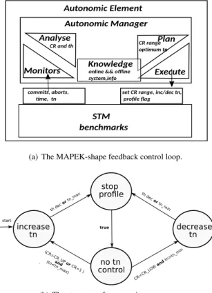
Figure 3(a) gives the structure of the complete platform which forms a MAPEK feedback control loop. The structure of the autonomic manager is shown in Figure 3(b). The autonomic manager, which can be also seen as the controller, is described as an automaton in the report. The automaton is composed of four states, and the program can only stay in one at each decision point.
STM benchmarks
commits, aborts, �me, tn
set CR range, inc/dec tn, profile flag
Autonomic Element Autonomic Manager
Monitors Execute Analyse
CR and th CR rangePlan op�mum tn
Knowledge
online && offline system,info
(a) The MAPEK-shape feedback control loop.
increase tn no tn control th dec or tn_max CR<CR _LOW and tn>tn _min (CR>C R_UP or CR=1 ) and ( tn<tn _max) . true start decrease tn th dec or tn_min stop profile
(b) The structure of autonomic manager
Figure 3: The feedback control loop of the simple model.
4.2.1 Control Objective
Under control theory terminology, the control objective of the feedback control loop is to maximize throughput and reduce the application execution time. This is achieved by controlling the level of paral-lelism to obtain the trade-off between the synchronization time and the computing time.
thread number 0
thr
oughput
local optimum point
global optimum point
10% variation
Figure 4: Throughput fluctuation. The throughput may continuously rise and descend before reaching the maximum point.
4.2.2 Inputs and Outputs
The inputs of the loop are commits, aborts and physical time (see Section 3.1 for definition). The output-s/actions are the optimum parallelism, the parallelism profile flag and the CR range setting.
4.2.3 Three Decision Functions
The control loop is activated at each decision point. Three decision functions cooperate to make decisions: a parallelism decision function, a CR range decision function and a profiling decision function. At each decision point as illustrated in Figure 3(b) one corresponding decision function reacts to make its decision. We firstly detail the parallelism decision function and the profiling decision function as they overlap with each other. Then we present the CR range decision function.
The automaton commences at state increase tn to increase the thread number, since the thread number is set to be the minimum at the starting point. In each parallelism profile interval, the parallelism can either continuously increase or decrease. The direction of parallelism regulation (increase or decrease) is determined by the profiling decision function. If the current throughput is greater than the previous throughput, one thread is awaken or suspended and the current throughput is recorded as the maximum throughput. The state transfers to stop profile when the current throughput is less than the maximum throughput. At the final decision point of a parallelism profile interval (state stop profile), the parallelism is set to be the value which yields the maximum throughput. A new CR range may be computed at the end of a parallelism profile interval, we will detail it later in this section. Then the automaton enters from state stop profile to state no tn control which corresponds to non-action interval in Figure 2. At each decision point of a non-action interval, the profiling decision function decides if a new parallelism profile interval is needed. More specifically, if the CR falls into the CR range, the program stays in no tn control state. Otherwise a boolean value is set indicating the direction of the parallelism regulation. Specifically, the automaton jumps into increase tn if CR is higher than the upper CR threshold or decrease tn if CR is lower than the lower CR threshold. It is worth noting that, In case the maximum value of the upper threshold is 100%, and the program CR is 100% (when only reads operation in the transactions or no conflicts among transactions), a higher parallelism to the program is assigned.
It is worth noting that the throughput often fluctuates before reaching the optimum value (shown in Figure 4). To prevent a parallelism profiling procedure from terminating at a local maximum throughput, parallelism profiling procedure continues until the throughput decreases over 10% of the maximum value (10% is an empirical value which can be tuned).
predict tn stop profile no tn control th dec (CR<C R_L OW and tn>tn_m in) ((CR>C R_UP or CR =1 ) and tn<tn_ma x) . verify OR true true true start CR range th inc
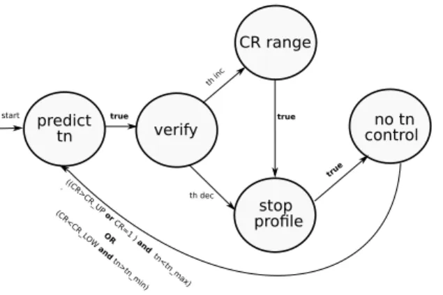
Figure 5: The controller of the probabilistic model described as an automaton. th in the figure stands for throughput and tn means the number of thread.
tn. A program still progresses in the same phase when its CR fluctuate within a certain range. Within the range the program produces its optimum throughput level. Therefore no parallelism regulation is required. However it is onerous to determine such a CR range offline, especially it is impossible to set a fixed CR range for some programs with online performance variation. Also, a constant CR range impedes programs to search its optimum parallelism. Therefore it becomes necessary to dynamically resolve a CR range. We add a CR range decision function. So at the end of a parallelism interval, a new CR range is prescribed. The function is activated at state stop profile. The two thresholds of the CR range are the CR values produced by running with one more or one less parallelism than the optimum one.
4.3
Feedback Control Loop of the Probabilistic model
The approach to manipulate one thread number at each decision point engages long profiling time which may slow down the program. This section presents a probabilistic model which predicts the optimum parallelism after one profile length based on the CR and current active thread number. The profiling procedure is similar to the simple model as shown in Figure 2, hence only the automaton is detailed in the section.
As illustrated in Figure 5, the automaton commences from predict tn state which yields an optimum parallelism. Then it unconditionally enters verify state to verify the correctness of the predicted paral-lelism where the predicted optimal paralparal-lelism is applied for the subsequent one profile length. The new parallelism is only applied when the throughput of the successive profile length is larger than the previ-ous throughput which leads to the state transfer to CR range state where a new CR range is prescribed. Otherwise the automaton enters stop profile state where the parallelism is switched back to the value before profiling and no new CR range is needed. Unlike the simple model, the probabilistic model re-quires an individual state to obtain the CR range. Simple model continuously increase and decrease the thread number until reaching the optimum value, therefore no additional state is needed to compute the CR range.
This model share the same inputs, outputs and control objective are as in the simple model. It also in-corporates three decision functions. As the CR range decision function and the profiling decision function are the same as that in Section 4.1, we only cover the parallelism decision function in this section.
4.3.1 Parallelism Decision Function
This section describes a probabilistic model which serves as the parallelism decision function. This probabilistic model however has its limitation, it is based on two assumptions:
• as every thread shows similar behaviour in our TM applications, we assume that the same amount of transactions are executed in the active threads during a fixed period,
• there is a large amount of transactions executed during the fixed period making the probability of conflicts between two transactions infinitely approaches a constant, thus the probability of one commit (see Section 3.1 for definition) infinitely approaches a constant.
Suppose during an application execution and within a fixed period L0, assuming that the average
length of transactions (including the aborted transactions and the committed transactions) is L , thus the
number of transactions N executed during L0can be expressed in equation (1).
N= n.L0
L = α.n (1)
Where n stands for the number of active threads during L0, N contains both aborts and commits, and
a=L0
L.
We assume that the probability of the conflicts p between two transactions is independent from the current active threads, thus independent from the number of active transactions. Therefore during the
L0period, one transaction can commit if it encounters no conflicts with other active transactions. The
probability of a commit can be expressed in Equation (2).
P(Xi= 1) = q(N−1) (2)
Where q = 1 − p, which stands for the probability of a commit between two transactions. However, the transactions executed in a sequence within the same thread do not cause conflicts among each other, the
probability of a commit in Equation (2) is lower than the reality. We suppose that during L0period, each
thread approximately execute the same number of transactions which is Nn. Therefore the number of
transactions causing conflict are reduced to N −Nn. So Equation (2) can be modified as in Equation (3).
P(Xi= 1) = q(N−
N
n) (3)
Equation 3 is correct only if there is a large amount of transactions executed during L0period making
the probability of conflicts p between two transactions infinitely approaches a constant, thus q infinitely approaches a constant%.
Under the terminology of probability theory, Xiis a random variable with Xi= 1 if the transaction i is
committed, Xi= 0 if i aborted. Xifollows a Bernoulli law of parameter q(N−
N n).
Let T represents the throughput. In a unit of time, the throughput can be also expressed as T = ∑ Xi
and CR can be expressed as CR = TN. As T is a random variable which follows a binomial distribution
B(N, q(N−Nn)). The expected value of T is therefore to be:
E[T ] = N.q(N−Nn)= αnqα(n−1) (4)
Hence
E[CR] = q(N−Nn)= qα(n−1) (5)
Equation (4) can be rewritten as a function from n to T as shown in Equation (6).
To obtain the value of n where the throughput can reach the maximum, we compute the derivation of Equation (6) as shown in Equation (7).
T0(n) = αqα(n−1)
+ α2nqα(n−1)ln(q) (7)
Therefore
T0(nopt) = 0 ⇔ αqα(nopt−1)+ α2noptqα(nopt−1)ln(q) = 0
⇔ qα(nopt−1).(α + α2n
optln(q)) = 0
⇔ α + α2n
optln(q) = 0
⇔ nopt= −α ln(q)1 (8)
Where noptstands for the optimum value of n which is the optimum thread number.
From Equation (5), we can obtain q = CR 1
α(n−1). Then Equation (8) can be rewritten as follows.
nopt= −
n− 1
ln(CR) (9)
Where noptstands for optimum thread number, n stands for the number of current active threads and
CRis the current commit ratio.
5
Implementation
There are two methods of collecting application profile information in a parallel program. One can employ a master thread to record the interesting information of itself. An alternative way is to collect the information from all threads. The first method requires little synchronization cost for information gathering but the obtained information may not represent the global view. Also the master thread must be active during the whole program execution which may make it terminate much earlier than the other threads, meaning that the fair execution time among threads can not be guaranteed. The later method may suffer from synchronization cost but the profile information gathered represent the global view. And more importantly, a fair execution time strategy can be employed among threads. We choose the second method. The synchronization cost of information gathering is negligible for most of our applications.
We have implemented a monitor to control the dynamic parallelism as well as the race condition. The monitor is a cross-thread lock which consists of the concurrent-access variables by threads. The major variables of the monitor are commits, aborts, two FIFO queues recording the suspended and active threads, the current active thread number, the optimum thread number and the throughput. There are three entry points of the monitor which is illustrated in Figure 6. The first entry point is upon threads initialization, where some threads are allowed to pass and the rest are suspended. Only two threads pass the entry point in the simple model and all the threads pass in the probabilistic model. The second entry point is upon transaction committing, where commits are accumulated and where the control functions take actions. The third entry point is upon a thread exiting, where one suspended thread is awaken when one thread exits.
Two metrics are often used to time the profile length: physical time and logic time. We choose logic time due to the fact that the size of transaction varies in various applications leading to the huge variation of execution time. Commits and aborts are two frequent meaningful events in TM and are good candidates to track the logic event. We choose to use the number of commits as the timing metric, as it is often a fixed value for an application. The choice of the profile length mainly depends on the total amount of transactions in an application. The applications with the same magnitude number of transactions share the same profile length. For instance, genome and vacation share the same profile length as the total
1 void control_func(time,commits,aborts)
2 {
3 ...
4 tn decision func;
5 CR range decision func;
6 profiling decision func;
7 ... 8 } 1 stm_thread_init(){ 2 ... 3 control_func(time,commits,aborts); 4 ... 5 } 1 stm_commit() { 2 ... 3 control_func(time,commits,aborts); 4 } 1 stm_thread_exit(){ 2 ... 3 control_func(time,commits,aborts); 4 ... 5 }
Figure 6: The three entry points of the monitor and the control functions. monitor in the figure is a cross-thread lock which includes the concurrent access variables by cross-threads. The codes are written in pseudo C. tn stands for active thread number.
Some benchmarks themselves such as genome and ssca2 incorporate multiple thread barriers which cause conflicts with the monitor, thus deadlock. We insert an additional function before thread barriers to avoid the deadlock. Once a thread encounters a barrier, it awakes one suspended thread. When all the thread have passed the barrier, the last thread sets the parallelism back to the optimal value.
A time overhead is added to each transaction when calling and releasing a monitor. The overhead caused by calling locks is negligible on the transaction with medium length or long length. But this overhead is significant for the transaction with a small number of operations. This is the case for intruder and ssca2. Such an overhead can be reduced through diminishing the frequency of calling the monitor. More specifically, the monitor is called every 100 commits rather than every commit.
To avoid thread starvation, we adopt round-robin thread scheduling to periodically awaken early sus-pended threads and put the running threads with the longest execution time to sleep. When a thread is awaken or suspended, it always awakes the one suspended at the earliest time or suspends the one run-ning for the longest time. We have implemented two different round-robin scheduling algorithms. A time stamp based round-robin and two FIFO queues. The time stamp method marks an explicit time line for each thread (the time when it is awaken, the time when it is suspended). While the FIFO gives a simple implementation but without explicit time line.
6
Performance Evaluation
In this section, we present the results from 6 different applications from STAMP [3] and two applications from EigenBench [8]. EigenBench and STAMP are the benchmarks that are widely used for perfor-mance evaluation of TM systems. The data set covers a wide range from short transaction length to long transaction length, long program execution time to short execution time, from high program contention to low contention. Table 1 presents the qualitative summary of each application’s runtime transactional char-acteristics: length of a transaction (number of instructions per transaction), execution time and amount of contention. The classification is based on the application with its static optimal parallelism. A trans-action with execution time between 10us and 1000 us is classified as medium-length. The contention between 30% and 60% is classified as medium. The execution time between 10 seconds and 30 seconds are classified as medium.
Application TX length Execution time Contention
EigenBench stable medium long medium
EigenBench online medium long medium
intruder short medium high
genome medium short high
vacation medium medium low
ssca2 short short low
yada medium medium high
labyrinth long long low
Table 1: Qualitative summary of each application’s runtime transactional characteristics. Tx length is the number of instructions per transaction. Execution time means the whole program execution time. Contention is the global contention of the application. The classification is based on the application with its optimal parallelism applied.
6.1
Platform
We evaluate the performance on a SMP machine which contains 4 processors with 6 cores each. Every two cores share a L2 cache (3072KB) and every 6 cores share a L3 (16MB) cache. This machine holds 2.66GHz frequency and 63GB RAM. We utilise TinySTM as our STM platform.
6.2
Benchmark Settings
We show two different data set of EigenBench. One with stable online behaviour and one with online variation. The two data set both incorporate medium-length transactions. As EigenBench does not experience online variation, we have modified its source code to enable online fluctuation. EigenBench include 3 different arrays which provide the shared transactional accesses (Array1), private transactional accesses (Array2) and non-transactional accesses (Array3). We vary the size of Array1 at runtime making the conflict rate vary among threads during execution. More specifically, within the first 40% amount of the transactions, the size of Array1 keeps the value given by the input file. From 40% to 70%, the array size is shrunk to be 16% of the original value and afterwards the size is set to be 33% of the original value. The main inputs of the both data sets are given in Figure 7.
We have tested 6 different applications from STAMP, namely intruder, ssca2, genome, vacation, yada and labyrinth. Two applications namely Bayes and Kmeans from STAMP are not taken into consideration in this report. As Bayes exhibits non-determinism [12]: the ordering of commits among
loops 16667 A1 35536 A2 1048576 A3 8192 R1 30 W1 30 R2 20 W2 200 R3i 10 W3i 30 R3o 10 W3o 10 NOPi 0 NOPo 0 Ki 1 Ko 1 LCT 0
(a) inputs for stable be-haviour loops 33333 A1 145530 A2 1048576 A3 8192 R1 30 W1 30 R2 20 W2 200 R3i 10 W3i 30 R3o 10 W3o 10 NOPi 0 NOPo 0 Ki 1 Ko 1 LCT 0
(b) inputs for online varia-tion
Figure 7: Two data sets of EigenBench inputs for 24 threads
threads at the beginning of an execution can drastically affect execution time. Kmeans owns too low contention, even running with the maximum parallelism, its CR is almost 100%. Hence there is little interest to employ runtime parallelism adaptation for this benchmark. The inputs of the six selected applications are detailed in Figure 8.
intruder -a8 -l176 -n109187
ssca2 -s20 -i1.0 -u1.0 -l3 -p3
genome -s32 -g32768 -n8388608
vacation -n4 -q60 -u90 -r1048576 -t4194304
yada -a15 -i inputs/ttimeu1000000.2
labyrinth -i random-x1024-y1024-z7-n512.txt
Figure 8: The inputs of STAMP applications.
6.3
Results
We firstly present the results of the execution time comparison between two autonomic parallelism adap-tation approaches and static parallelisms. Followed that we illustrate the online parallelism change from the two models. To verify that the runtime thread number change corresponds to the program behaviour change, we present the online throughput change of the static and dynamic parallelisms. The maximum parallelism is 24 which is the number of the available cores. The minimum parallelism is restricted to be
2. All the applications are executed 10 times and results are the average execution time. We also show the probabilistic variance to indicate stability of the autonomic approaches.
Figure 9 and Figure 10 illustrate the execution time comparison with different static parallelisms and adaptive parallelisms of EigenBench and STAMP. The dots represent the execution time with different static parallelism. The solid black line stands for execution time with the simple model and the dashed red line gives the execution time with the probabilistic model.
thread number
e
x
ecution time (second)
● ● ● ● ● ● ● ● ● ● ● ● 0 4 8 13 18 23 28 33 38 43 48 53 58 63 68 2 4 6 8 10 12 14 16 18 20 22 24 simple probabilistic (a) stable thread number e x
ecution time (second)
● ● ● ● ● ● ● ● ● ● ● ● 0 10 20 30 40 50 60 70 80 90 110 130 2 4 6 8 10 12 14 16 18 20 22 24 simple probabilistic (b) online variation
Figure 9: Time comparison of EigenBench on static and adaptive parallelisms. The dots represent the execution time with different static parallelism.
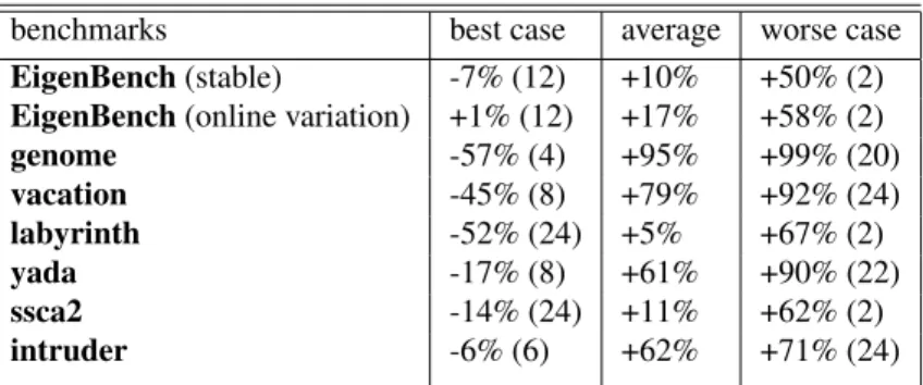
According to Figure 9 and Figure 10, our adaptive models outperform the performance of the major-ity of the static parallelisms. The probabilistic model shows better performance on applications: Eigen-Bench, genome, vacation, labyrinth against the simple model, but it indicates a performance degrada-tion on yada, ssca2 and intruder against the simple model. Table 2 and Table 3 detail the performance comparison. We compare the results with best, average and worst case to show that our models are able to outperform the performance of static parallelism if an unknown application is given. The digits in the brackets are the static thread numbers which give the best performance and the worst performance respectively.
benchmarks best case average worse case
EigenBench (stable) -7% (12) +10% +50% (2)
EigenBench (online variation) +1% (12) +17% +58% (2)
genome -57% (4) +95% +99% (20) vacation -45% (8) +79% +92% (24) labyrinth -52% (24) +5% +67% (2) yada -17% (8) +61% +90% (22) ssca2 -14% (24) +11% +62% (2) intruder -6% (6) +62% +71% (24)
Table 2: Performance comparison on applications with simple model. The performance is compared with the minimum, average and the maximum value of the static parallelisms. The digits in the bracket are the thread numbers of the best case and the worst case.
Table 4 presents the variance of the ten-time executions, as well as the average value on simple and probabilistic models. As shown in the table, the turbulence of the ten-time executions is low.
Figure 11 and Figure 12 elucidate the runtime parallelism variation with simple and probabilistic model. The simple model spends some time before reaching the optimum parallelism which gives stairs
thread number
e
x
ecution time (second)
● ● ● ● ● ● ● ● ● ● ● ● 0 2 4 6 8 11 14 17 20 23 26 29 32 35 38 2 4 6 8 10 12 14 16 18 20 22 24 simple probabilistic (a) intruder thread number e x
ecution time (second)
● ● ● ● ● ● ● ● ● ● ● ● 0 1 2 3 4 5 6 7 8 9 11 13 15 17 19 2 4 6 8 10 12 14 16 18 20 22 24 simple probabilistic (b) ssca2 thread number e x
ecution time (second)
● ● ● ● ● ● ● ● ● ● ● ● 0 40 80 130 180 230 280 330 380 430 480 530 2 4 6 8 10 12 14 16 18 20 22 24 simple probabilistic (c) genome thread number e
xecution time (second)
● ● ● ● ● ● ● ● ● ● ● ● 0 10 30 50 70 90 110 130 150 170 2 4 6 8 10 12 14 16 18 20 22 24 simple probabilistic (d) vacation thread number e
xecution time (second)
● ● ● ● ● ● ● ● ● ● ● ● 0 10 20 30 40 50 60 70 80 90 100 110 2 4 6 8 10 12 14 16 18 20 22 24 simple probabilistic (e) yada thread number e
xecution time (second)
● ● ● ● ● ● ● ● ● ● ● ● 0 10 30 50 70 90 110 130 150 170 2 4 6 8 10 12 14 16 18 20 22 24 simple probabilistic (f) labyrinth
Figure 10: Time comparison for STAMP on static and adaptive parallelism. The dots represent the execution time with different static parallelism.
in the figure. The probabilistic model react immediately once the contention or phase change is detected. As less time spent to reach the optimum parallelism, the performance by probabilistic model usually outperforms the simple model. In Figure 11, simple model and probabilistic model produce different parallelism on EigenBench. This is because certain parallelisms yield similar throughputs which can be seen in Figure 13. For instance in Figure 13(b), on the third phase 8, 16 and 24 thread number produce very similar throughput. genome experiences three phased at runtime. The first phase is short (two or three profile lengths) which contains both read and write operations. During the second phase, the transactions only contain read operations resulting in 100% of CR, hence the maximum parallelism is applied. The third phase brings high contention to the program, hence low parallelism. intruder shows an abrupt thread number fluctuation with probabilistic model due to the sudden CR change, but simple model smooths the abrupt fluctuation. ssca2 has low CR with trivial but frequent change and its performance stays stable after 8 thread number. In Figure 12(b), the simple model brings frequent parallelism variation due to the frequent CR change. In contrary, the probabilistic model does not give frequent parallelism change, as CR is high which makes the model always predict the maximal thread number. Figure 12(e), the parallelism shows periodically change from both models. yada has very high contention with its average CR lower than 10%. Although CR is low and its variation is relatively small, it varies periodically leading to the models to adapt the parallelism periodically.
Figure 13 and Figure 14 elucidate the online throughput behaviour under different static parallelism as well as the adaptive parallelisms for EigenBench and STAMP. The autonomic parallelism adaptation aims to regulate the parallelism which retains throughput at the optimum level at each phase. Ideally the throughput should rival the one with the static parallelism which achieves the maximum through-put. Therefore the runtime thread number adaptation is correct if the corresponding throughput always
benchmarks best case: average worse case
EigenBench (stable) +5% (12) +20% +56% (2)
EigenBench (online variation) +3% (12) +19% 59% (2)
genome +3% (4) +95% +99% (20) vacation -14% (8) +83% +94% (24) labyrinth +8% (24) +42% +80% (2) yada -31% (8) +56% +89% (22) ssca2 -22% (24) +5% +60% (2) intruder -32% (6) +52% +64% (24)
Table 3: Performance comparison on applications with probabilistic model. The performance is compared with the minimum, average and the maximum value of the static parallelisms. The digits in the bracket are the thread numbers of the best case and the worst case.
benchmarks (unit=second) simple model probabilistic model
EigenBench (stable) 1.78|34.03 0.39|33.30
EigenBench (online variation) 1.69| 56.81 0.92|55.82
genome 1.21|7.20 0.21|4.51 vacation 9.06|13.56 1.52|10.66 labyrinth 2.86|56.32 1.59|34.27 yada 0.01|10.78 0.11|12.09 ssca2 0|7.03 0|7.47 intruder 0.57 |11.27 0.91|14.12
Table 4: The variance and average of 10-time executions on simple and probabilistic models. The value before the line is the variance (the lower the better), the other one is the average value.
approaches the optimum throughput produced by the static parallelism at each phase.
7
Discussion
The overhead of our approaches mainly originate in the following aspects:
1. Thread migration. This can introduce a large overhead especially when the parallelism is adapted at runtime, as threads keep migrate among different cores.
2. The choice of the thread number to manipulate at each parallelism profile length. We simply choose to manipulate one thread number at each decision point (in the simple model) which delays the procedure to reach the maximum parallelism.
3. The choice of throughput variation rate. Parallelism profiling procedure continues even if the cur-rent throughput is slightly lower than the recorded maximum throughput in order to avoid the procedure to terminate at a regional maximum point. We choose 10%, which is an empirical value, as variation between the current throughput and the maximum throughput.
4. The cost of calling locks. Two factors contribute to this cost: the operation of obtaining and releas-ing the lock and the time spent contendreleas-ing for the lock. The later cost increases significantly with more active thread number and give huge imparts on the applications with short-length transaction. The cost of calling a lock is insignificant in our approaches.
logic time (1K commits) thread n umber 0 1 2 3 4 5 6 7 8 9 10 11 12 13 14 15 16 17 18 19 20 21 22 23 24 0 10 20 30 40 50 60 70 80 90 100 110 120 130 140 150 160 170 180 190 200 210 220 230 240 250 260 270 280 290 300 310 320 330 340 350 360 370 380 390 400 410 simple probabilistic (a) stable
logic time (1K commits)
thread n umber 0 1 2 3 4 5 6 7 8 9 10 11 12 13 14 15 16 17 18 19 20 21 22 23 24 0 50 110 180 250 320 390 460 530 600 670 740 810
thread variation online
simple probabilistic
(b) online
Figure 11: Runtime thread number variation by simple and probabilistic model. The solid black line and the dashed red line is by simple model and probabilistic model respectively.
logic time (300K commits)
thread n umber 0 1 2 3 4 5 6 7 8 9 10 11 12 13 14 15 16 17 18 19 20 21 22 23 24 0 2 4 6 8 10 12 14 16 18 20 22 24 26 28 30 32 34 36 38 40 42 44 46 simple probabilistic (a) intruder
logic time (10K commits)
thread n umber 0 1 2 3 4 5 6 7 8 9 10 11 12 13 14 15 16 17 18 19 20 21 22 23 24 0 100 200 300 400 500 600 700 800 900 1000 1100 1200 1300 1400 1500 1600 1700 1800 1900 2000 2100 2200 2300 simple probabilistic (b) ssca2
Additionally, the choice of profile length may degrade application performance. A short profile length does not provide sufficient information to the profiling algorithm to search the best parallelism, while a long length wastes time in parallelism profiling where the program executes under a sub-optimum parallelism.
The simple model demonstrates an effective way to control programs with medium-length transac-tions (e.g.genome) and short-length transactransac-tions (e.g. intruder). However it gives a heavy overhead against the best case for the application with long-length transactions, as simple model only manipulates one thread number at each decision point. However this eludes the possibility of skipping a certain
op-logic time (10K commits) thread n umber 0 1 2 3 4 5 6 7 8 9 10 11 12 13 14 15 16 17 18 19 20 21 22 23 24 0 10 20 30 40 50 60 70 80 90 100 110 120 130 140 150 160 170 180 simple probabilistic (c) genome
logic time (10K commits)
thread n umber 0 1 2 3 4 5 6 7 8 9 10 11 12 13 14 15 16 17 18 19 20 21 22 23 24 0 10 20 30 40 50 60 70 80 90 100 110 120 130 140 150 160 170 180 190 200 210 220 230 240 250 260 270 280 290 300 310 320 330 340 350 360 370 380 390 400 410 420 430 simple probabilistic (d) vacation
logic time (10K commits)
thread n umber 0 1 2 3 4 5 6 7 8 9 10 11 12 13 14 15 16 17 18 19 20 21 22 23 24 0 10 20 30 40 50 60 70 80 90 100 110 120 130 140 150 160 170 180 190 200 210 220 230 240 250 simple probabilistic (e) yada
logic time ( 15 commits)
thread n umber 0 1 2 3 4 5 6 7 8 9 10 11 12 13 14 15 16 17 18 19 20 21 22 23 24 0 2 4 6 8 10 12 14 16 18 20 22 24 26 28 30 32 34 36 38 40 42 44 46 48 50 52 54 56 58 60 62 64 66 68 70 simple probabilistic (f) labyrinth
Figure 12: Runtime thread number variation by simple and probabilistic model. The solid black line and the dashed red line is by simple model and probabilistic model respectively.
timum parallelism while profiling. The application always starts with two threads activated rather than the maximum value to avoid excessive contention, as high contention may prevent a program from pro-gressing. However this setting imposes long parallelism profiling time on the applications which require a high parallelism, this is especially true for labyrinth that requires maximum thread number to achieve its maximum throughput. Such an overhead is difficult to be compensated by the performance improve-ment brought by the optimum parallelism. genome requires the maximum thread number in the second phase but only needs minimal parallelism in the third phase leading to a high overhead which originates in the slow parallelism descending procedure. Such overhead is especially large when the application is
commits (1k) throughput( ktx/s) 0 1 2 3 4 5 6 7 8 9 10 11 12 13 14 15 16 17 18 19 0 10 20 30 40 50 60 70 80 90 100 110 120 130 140 150 160 170 180 190 200 210 220 230 240 250 260 270 280 290 300 310 320 330 340 350 360 370 380 390 400 410 online throughput variation
● ● ● ● ● ● ● ● ● 2threads 4thread 8threads 16threads 24threads simple probabilistic (a) stable commits (1k) throughput( ktx/s) 0 10 20 30 40 0 100 200 300 400 500 600 700 800 online throughput variation
● ● ● ● ● ● ● ● ● 2threads 4thread 8threads 16threads 24threads simple probabilistic (b) online
Figure 13: Online throughput variation of EigenBench. The red line with crosses and the sky blue line with circles is the simple model and probabilistic model respectively.
commits (300k) throughput( ktx/s) 0 100 200 300 400 500 600 700 800 900 1000 1100 1200 1300 1400 1500 1600 1700 1800 1900 2000 2100 2200 2300 2400 2500 2600 2700 2800 2900 0 2 4 6 8 10 12 14 16 18 20 22 24 26 28 30 32 34 36 38 40 42 44 46 ● ● ● ● ● ● ● ● ● ● ● ● ● ●● ● ●● ●● ● ● ● ● ● ●● ● ● ● ● ● ● ● ● ●● ● ● ● ● ● ● ● ● ● 2threads 4thread 8threads 16threads 24threads simple probabilistic (a) intruder commits (10k) throughput( ktx/s) 0 1000 2000 3000 4000 5000 6000 7000 8000 9000 10000 11000 12000 0 100 200 300 400 500 600 700 800 900 1000 1100 1200 1300 1400 1500 1600 1700 1800 1900 2000 2100 2200 2300 ● ● ● ● ● ● ●● ● 2threads 4thread 8threads 16threads 24threads simple probabilistic (b) ssca2
experiencing high contention.
The probabilistic model predicts the parallelism in one step which diminishes the profiling time and gives better performance than the simple model in most of the cases. However the probabilistic model starts with the maximum parallelism to guarantee enough amount of concurrent transactions. And such a setting delivers a large time spending in the first profile length. In addition, the probabilistic model has the potential risk of overreacting to the phase variation as only one profile length is required for prediction. On top of that, the probabilistic model is based on two assumptions:
commits (10k) throughput( ktx/s) 0 1000 2000 3000 4000 5000 6000 0 10 20 30 40 50 60 70 80 90 100 110 120 130 140 150 160 170 180 ● ● ● ● ● ● ●● ● 2threads 4thread 8threads 16threads 24threads simple probabilistic (c) genome commits (10k) throughput( ktx/s) 0 100 200 300 400 500 600 700 0 10 20 30 40 50 60 70 80 90 100 110 120 130 140 150 160 170 180 190 200 210 220 230 240 250 260 270 280 290 300 310 320 330 340 350 360 370 380 390 400 410 420 430 ● ● ● ● ● ● ●● ● 2threads 4thread 8threads 16threads 24threads simple probabilistic (d) vacation commits (10k) throughput( ktx/s) 0 100 200 300 400 500 0 10 20 30 40 50 60 70 80 90 100 110 120 130 140 150 160 170 180 190 200 210 220 230 240 250 online throughput variation
● ● ● ● ● ●● ● ● 2threads 4thread 8threads 16threads 24threads simple probabilistic (e) yada commits (15) throughput(tx/s) 0 10 20 30 40 50 60 70 80 90 100 110 120 130 140 150 160 170 180 190 200 210 220 0 2 4 6 8 10 12 14 16 18 20 22 24 26 28 30 32 34 36 38 40 42 44 46 48 50 52 54 56 58 60 62 64 66 68 ● ● ● ●●● ● ●●●●●●● ● ●●● ● ● ● ●●● ● ● ● ● ●● ● ● ● ● ● ● ● ● ● ● ● ● ● ● ● ● ● ● ●● ● ●● ● ● ● ● ● ● ● ● ● ●● ● ● ● ● 2threads 4thread 8threads 16threads 24threads simple probabilistic (f) labyrinth
Figure 14: Online throughput variation. The red line with crosses and the sky blue line with circles is the simple model and probabilistic model respectively.
• the same amount of transactions are executed in the active threads during a fix period.
• if there is a large amount of transactions executed during the fixed period making the probability of conflicts p between two transactions infinitely approaches a constant, thus q infinitely approaches a constant.
8
Conclusion and Future Work
In this report, we have investigated two autonomic parallelism adaptation approaches on a STM system (TinySTM). We examined the performance of different static parallelisms and conclude that runtime reg-ulation of parallelism is crucial to the performance of STM systems. We then presented our approaches and compared their performance with static parallelisms. We introduced feedback control loops to au-tonomically manipulate parallelism. We then analysed the implementation overhead and discussed the advantages as well as limitation of our work.
Apart from inappropriate parallelism, thread migration among cores impacts on system performance and cause performance degradation too. We plan to investigate the issue and design additional loops which will work together with the current loops to control the thread affinity and further enhance system performance.
Acknowledgement
This work has been partially supported by the LabEx PERSYVAL-Lab (ANR-11-LABX-0025-01) funded by the French program Investissement d’avenir.
References
[1] M. Ansari, C. Kotselidis, K. Jarvis, M. Luján, C. Kirkham, and I. Watson. Adaptive concurrency control for transactional memory. In MULTIPROG ’08: First Workshop on Programmability Issues for Multi-Core Computers, January 2008.
[2] M. Ansari, C. Kotselidis, K. Jarvis, M. Luján, C. Kirkham, and I. Watson. Advanced concur-rency control for transactional memory using transaction commit rate. In Proceedings of the 14th International Euro-Par Conference on Parallel Processing, Euro-Par ’08, pages 719–728, Berlin, Heidelberg, 2008. Springer-Verlag.
[3] C. Cao Minh, J. Chung, C. Kozyrakis, and K. Olukotun. STAMP: Stanford transactional applica-tions for multi-processing. In IISWC ’08: Proceedings of The IEEE International Symposium on Workload Characterization, September 2008.
[4] P. Damron, A. Fedorova, Y. Lev, V. Luchangco, M. Moir, and D. Nussbaum. Hybrid transactional memory. SIGPLAN Not., 41(11):336–346, Oct. 2006.
[5] D. Didona, P. Felber, D. Harmanci, P. Romano, and J. Schenker. Identifying the optimal level of parallelism in transactional memory applications. In V. Gramoli and R. Guerraoui, editors, Net-worked Systems, volume 7853 of Lecture Notes in Computer Science, pages 233–247. Springer Berlin Heidelberg, 2013.
[6] P. Felber, C. Fetzer, and T. Riegel. Dynamic performance tuning of word-based software transac-tional memory. In Proceedings of the 13th ACM SIGPLAN Symposium on Principles and practice of parallel programming, PPoPP ’08, pages 237–246, New York, NY, USA, 2008. ACM.
[7] M. Herlihy and J. E. B. Moss. Transactional memory: architectural support for lock-free data structures. SIGARCH Comput. Archit. News, 21(2):289–300, May 1993.
[8] S. Hong, T. Oguntebi, J. Casper, N. Bronson, C. Kozyrakis, and K. Olukotun. Eigenbench: A simple exploration tool for orthogonal tm characteristics. In Workload Characterization (IISWC), 2010 IEEE International Symposium on, pages 1–11, Dec 2010.
[9] M. C. Huebscher and J. A. McCann. A survey of autonomic computing — degrees, models, and applications. ACM Comput. Surv., 40(3):7:1–7:28, Aug. 2008.
[10] J. O. Kephart and D. M. Chess. The vision of autonomic computing. Computer, 36(1):41–50, Jan. 2003.
[11] K. Ravichandran and S. Pande. F2c2-stm: Flux-based feedback-driven concurrency control for stms. In Parallel and Distributed Processing Symposium, 2014 IEEE 28th International, pages 927–938, May 2014.
[12] W. Ruan, Y. Liu, and M. Spear. Stamp need not be considered harmful. In 9th ACM SIGPLAN Workshop on Transactional Computing, Salt Lake City, March 2014.
[13] D. Rughetti, P. Di Sanzo, B. Ciciani, and F. Quaglia. Machine learning-based self-adjusting con-currency in software transactional memory systems. In Modeling, Analysis Simulation of Computer and Telecommunication Systems (MASCOTS), 2012 IEEE 20th International Symposium on, pages 278–285, Aug 2012.
Contents
1 Introduction 3
2 Contribution 3
3 Background and Related Work 3
3.1 Transactional Memory . . . 4
3.2 Autonomic Computing . . . 4
3.3 Related Work . . . 5
4 Control of Autonomic Parallelism Adaptation 5 4.1 Overview of the Profiling Algorithm . . . 6
4.2 Feedback Control Loop of the Simple Model . . . 7
4.2.1 Control Objective . . . 7
4.2.2 Inputs and Outputs . . . 8
4.2.3 Three Decision Functions . . . 8
4.3 Feedback Control Loop of the Probabilistic model . . . 9
4.3.1 Parallelism Decision Function . . . 10
5 Implementation 11 6 Performance Evaluation 13 6.1 Platform . . . 13 6.2 Benchmark Settings . . . 13 6.3 Results . . . 14 7 Discussion 17
Inovallée BP 105 - 78153 Le Chesnay Cedex inria.fr