Designing Equitable Merit Rating Plans

--

~ ~

~

~

~

~ ~

~ ~ ~

-~

S5_,1

<G:

: il

. 0

:

: 00 \; ::

r

i: ::::--:

'a S

t

f~-

rlworking

:papc

er. -

;

0 ffI:

f

f..0.:.ff:. ff 0

...-

..

::

:-

*

:

a:

;

: :

:000:

:0000000;000

00000

0

0

-0

0:0

|fff: 0000~~~~~~~~

''' ",'_'_,, ' ''.' '' " "-,. ,_'',, '' '' ' '''' '.1 D"...E 1 ' '"

MAg,,,,,SACHUE

_WDO

_Mf

_:-i

TTS:,

_I,

INSTITUwTt,0

,-B.:i

-1~~·1~~~·73--

E4

X

· · ,~~~~!B·~~I-::-·-~A

f.

f

·:·

..II' · · · _{I --:.} -:.··..I -·---.··: . .-i-i *; _:· · : :.·'·..-.-r ;.-.. I'_.1 · · :.:. · · ··· ' ·: ., ·- -- - - .: - ·:-: .·: · · ; · ·

Designing Equitable Merit Rating Plans* by

Joseph Ferreira, Jr.**

OR-057-76 August 1976

All rights reserved. No part of this manuscript may be reproduced in any form without the written permission of the author.

Presented at 1976 annual meeting of the American Risk and Insurance Associ-ation, Boston, Massachusetts, August 16, 1976.

The author acknowledges the financial support, in part, of the MIT Class of 1972 Career Development Chair, the Massachusetts Automobile Rating and Accident Prevention Bureau, and the Massachusetts Division of Insurance. Associate Professor of Urban Studies and Operations Research currently on leave at the State Rating Bureau of the Massachusetts Division of Insurance. l

DESIGNING EQUITABLE MERIT RATING PLANS

Table of Contents

1. The Purpose of Merit Rating

2. Modeling the Effects of Merit Rating

3. Typical Merit Rating Plans and Model Parameters

4. An Illustrative Example

5. Conclusions and Implementation Issues

References 1 7 11 15 25 27

Designing Equitable Merit Rating Plans by

Joseph Ferreira, Jr.

Throughout the United States it is common practice for automobile insurance premiums for a particular policy to vary depending upon the driver class and geographic location of the policyholder as well as the type and number of

vehicles covered by the policy. In addition, most states also permit so-called "merit rating" plans whereby each policyholder's annual premium is adjusted up or down depending upon the insured's claims experience and traffice viola-tion record during previous years. Although these merit rating plans may be viewed as a special type of risk classification, the rationale underlying their use is quite different from the justification for driver class and territory differentials. This paper develops a methodology for evaluating merit rating plans that are used in conjunction with other risk classification

criteria. A theoretically equitable merit rating plan is designed and com-pared with plans commonly used throughout the country. The differences are striking, especially among high risk classes. For example, most typical merit rating plans overcharge good drivers in high risk classes -- often by more than 25%.

1.0 The Purpose of Merit-Rating

The popular rational behind merit-rating is straightforward: Merit-Rating keeps "good" drivers from subsidizing "bad" drivers and, because having any accident or traffic violation means higher rates, it promotes safe driving and

-2-deters motorists from having accidents and filing insurance claims. In the ideal situation where the "bad" drivers are readily identifiable, and the

deterrent effect is sizable merit-rating would indeed work well. Unfortunately, those who have--or even cause--accidents during a particular year are not always the "worst" drivers. A generally "good" driver whose rare instance of misjudg-ment causes an accident, must pay significantly higher premiums for several sub-sequent accident-free years. Furthermore, the plan might not save "good" drivers much money, since the vast majority of drivers are accident-free during any

particular year. Unless the deterrent effect were substantial, accident-free drivers would pay only 5% or 10% less with merit-rating than without, whereas accident-involved drivers might pay 100% to 500% more.

Before embarking on a mathematical discussion of merit-rating some notation and a non-technical discussion with help identify the important issues and trade-offs. For simplicity, let us focus on a particular line of auto insurance--such as collision coverage--and a standard policy for the actual cash value of a single private passenger vehicle of a particular age and value with, say, a

$100. deductible. In pricing such a policy one would like to consider the losses and a variety of

that might arise/other expense, profitability, marketing and competitive factors. Since we are primarily interested in variations in premiums that are at least

theoretically related to expected losses, we shall focus only on the "pure premium" component--that portion of earned premium that is expected to cover losses and loss adjustment expenses that can be associated with particular claims.*

If, as is typically the case in ratemaking, these other factors are expressed as a percentage of pure premium, the distinction between pure premium and total premium affects only a scaling factor.

-3-Classification schemes and merit rating plans try to distinguish policy-holders with relatively high and low loss potential. The differences might arise from driving behavior or from a host of exposure or driving environment

factors. Since accidents are rare events for virtually all inidividual motorists, one also recognizes that chance plays a large role in the timing of accidents.

Merit rating proceeds one step further and assumes that the loss potential associated with a policy is approximately constant from one year to the next*

(as long as the vehicle usage and driver characteristics remain unchanged). Hence those policyholders--within a driver class and territory--who drive poorly and had (or caused) accidents in the past are those most likely to generate losses in the future.

If we could characterize by a one-dimensional variable the loss potential of any individual policyholder, then one could envision a histogram such as that in Figure l of the loss potential among all policyholders of a particular com-pany or within a given state. In Figure 1, I have arbitarily specified the average loss potential to be $100,** and have drawn a histogram with a long right tail and many policies with below average loss potential.***

We would not expect the histogram to be very concentrated around the

average figure of $100 since class and territory distinctior are expected to be useful in distinguishing policyholders with relatively high and low loss potentials.

Note that class and territory distinctions alone do not require this strict an assumption--an entire classification group might have similar experience from one year to the next even if those within the group with above average loss potential one year were the drivers with below average loss potential the next year.

In Massachusetts most annual premiums for collision insurance amount to con-siderably more than $100. A typical Massachusetts policy holder in 1975 with, say, a new $4,000 car paid more than $150 for $200 deduction Collision coverage.

Histograms with this shape are commonly used in characterizing auto insurance risks. The rationale will become more apparent shortly.

//l sl)

Y'O jwi O

F

Z

oss

_{l -e, z}

_L

C /a rX · ,

Y )

Fl',gv t,

2

I

AVI

/')/C'

c)

you

30

aO-10 Q,

1y

K\

K

_ _ 2 s-_ · ., --CIIIIIIIIC( I l , - = ' B ! _{/cc- /;o /-/'O 16}

I

I

-5-Conceivably, an ideal 2 class by 2 territory scheme might divide the policy-holders in Figure 1 into the 4 non-overlapping subgroups as shown in Figure 2a. What is much more likely to occur is shown in Figure 2b. Each of the 4 class and territory subgroups is more concentrated* around the subgroup average than the composite histogram in Figure 1 but not as sharply concentrated as the ideal case in Figure 2a. Figure la situations are unlikely since age, sex, town of residence and other such characteristics are unlikely to explain all the differences in loss potential among policyholders.

Note also that the histogram refers to loss potential and not actual losses. The $100 average loss potential results from a combination of claim frequencies that average 1 every 6 to 10 years and claim costs that might run into the

thousands. Hence the majority of policyholders at each loss potential level will have no losses during any one year. But we expect those policyholders with the higher loss potential to constitute a disproportionately large share of those policyholders with some losses during year. The more pronounced this effect is, the better merit rating will work.

Using merit rating in addition to class and territory distinctions is least appropriate for the Figure 2a type of situation. In this case, all policyholder in each class and territory subgroup have the same loss potential and should ideally pay the same premium. Those within a subgroup who have losses during one year are not more likely to have losses again in the future and should not be merit rated.** Merit rating will be most useful when class

*

In subsequent sections we shall define more precisely a measure of concentration. Merit Rating might still be considered if it resulted in a large enough deterrent effect to outweigh this inequitable cost redistribution whereby those with acci-dents subsidize those without.

'-I '4 11 t ,.L 11. w

4z

N ---

~

.. ---A L Lj LA %

Ilttz

d · · r-~~~~~~r- i / 4 · a' c r 4 74t a~ ,_{NA~ -I}

~i

e2

. 0_{3- I I} J- -L U -4- - -Q -'4 It ·-``

E

L

K

.4: I-it -4 *2S cv fs

V

I _IGj

L

1

,

o 'Y

C

Y>

2Q

o - V 0L IN ' ' . o 3r _5 0

a

04Z 3 -4~ . .3

d

i

Z;

' J f~J

4,

Za

---11 0 0 '1- c 0 1 I Q 'r 1 1 .b Q Im 4~p~

rl,

- --Z C:~

C-z j

11I 7 11I

-and territory categories do not sharply differentiate policyholderswith high and low potential.

The remainder of the paper explores these issues in more detail using a mathematical model of accident involvement. Using the model, it is possible to estimate within-class variations in loss potential, develop a theoretically appropriate merit rating plan, and compare it with plans currently in use.

2.0 Modeling the Effects of Merit Rating

Theoretical work concerning strategies for rating various drivers has come from actuaries (Casualty Actuarial Society, 1960). The compound Poisson acci-dent model that will be used here to estimate the effects of merit-rating plans is well known among actuaries (Seal, 1969). However, the actuarial work has been, quite naturally, oriented toward the needs of the insurance companies and not toward the policyholder or regulatory agency. As a result, their work has been concerned with the annual pricing of risk classes on the basis of accumulated

loss experience, or has been oriented toward the use of compound Poisson and Markov models in the investigation of solvency questions, the design of balanced

risk-classification systems, and the study of related financial and economic questions. Actuarial models have seldom been used to examine in any detail the net redistribution of premium costs among motorists with different loss potential that would result after several year's operation of proposed merit-rating schemes.

In an earlier paper (Ferriera, 1974), I outlined the basic methodology for studying the long term effects of merit rating plans on individual motorists. But the earlier work did not consider the problem of using merit rating in con-junction with driver class and territory classifications.

-8-To model the claims experience of individual policyholders, we assume that an individual policy's loss potential Li can be expressed as the product

Li ' r i * 8i (1)

whew s_i and ri are independent random variables corresponding to the policy s expected claim frequency and claim severity respectively. For ease of exposi-tion we assume further that individual policies differ only with respect to claim frequency.

To estimate when and how often individual motorists are involved in acci-dents, assume a compound Poisson accident model commonly employed by actuaries and industrial safety researchers for more than half a century (Seal, 1969). Accordingly, the conditional probability that a policy with claims likelihood*

r is involved in i accidents during T years follows a Poisson distribution

~iiT~r

= -rTrTi

P (ilT,r) = (rT) e /i!. (i = 0,1,2,... ) (2)

Different policies.may have different claims likelihoods and the distribution of r values among all policies is approximated by a two-parameter gamma-1 function

(a Pearson Type III distribution)

f(rlk,k/m) = [(k/m)/r(k)](rk/m) k - e , r > 0) (3)

We use the term claims likelihood rather than claims frequency since the former refers to an unobserved characteristic of an individual policy whereas a claims

frequency commonly implies the observed average claims rate of a class and/or territory subgroup of policies.

-9-in terms of two nonnegative parameters k and m that may be estimated from sample driver-accident records. The gamma-1 family is rich and its use here is particularly desirable, since it is the natural conjugate family for Poisson sampling and facilitates a Bayesian approach toward updating claims likelihood estimates. The parameter m may be interpreted as the overal average accident rate. The k parameter affects the shape of the distribution. Since the variance of r equals mk, the coefficient of variation is 1/k and the distribution in more concentrated for larger values of k. For k = 1.00, a simple negative

exponential distribution results. To account for class and territory differences, the k and m parameters in (2) may be considered functions of the class and

territory characteristics for the collection of policies being considered.* This model is sometimes referred to as an accident-proneness model since it allows some policies to have consistently higher claims likelihoods than others, but assumes that an individual policy has a characteristic claim likelihood that is essentially unchanged from one year to the next. Simce the accuracy of

such a model has been considered at length elsewhere,** itis not reviewed here. One goodness-of-fit test is presented in the next Section.

If we adopt a Bayesian interpretation of the compound Poisson accident model, then a policy's claims history may be used to predict future experience.

Strictly speaking, a weighted sum of gamma distributions is no longer a gamma function. However, the gamma assumption need only be approximately correct since the exact shape of the claims likelihood distributions is not important to the analysis.

Arbous and Kerrich (1951) discuss in detail the application to accident process-es in general. Seal (1969) reviews actuarial usprocess-es and Ferreira (1971) reports detailed tests of the model using California driver accident data.

- 10

-Since the gamma-1 family is the natural conjugate for Poisson sampling, the

posterior density function for the claims likelihood of a policy with y accidents in t years is again a gamma-l function

f"(rly,t) = f'(rj(k + y), (k/m) + t). (4)

The expected value of this posterior distribution is (k + y)/((k/m) + t) whereas the mean of the prior was simply m.

This relation suggests a simple scheme for merit rating--charge policy i a premium

k + i

Ri(k,m,y,t) = C * Sj h (5)

m+t

m + t

if the policy had yi accidents during the last t years, where C is a loading factor to reflect overhead, profitability, etc., Sj is the average claim cost for policies with class/territory combination , and k and m are the para-meters of the claim likelihood distribution estimated for class/territory com-bination j. Note that (5) implies a linear relation between R and yi so that each claim during the t years adds an additional surcharge of C Sj/((k/m) + t) dollars to the premium.

If merit rating had a deterrent effect, the estimate in (5) might be high depending upon the extent to which the marginal cost of a claim affects a policy's claims likelihood in the future. We shall assume that, whatever deterrent

effect arises, it is not very sensitive to the differences in the surcharges for accidents among the plans we shall consider but only to the fact that claims history has some effect on future premiums.

- 11

-Another simplifying assumption that facilitates exposition without loss of generality is that we shall consider merit rate based only on claims ex-pefiende and not on traffic violation convictions as well.*

3.0 Typical Merit Rating Plans and Model Parameters

In most states, polices are assigned points depending upon the number of chargeable accident claims or traffic violation convictions they have had during the previous three years. These points are then used to adjust the policies rating factors. The rating factor for a particular class of policy is the ratio of the premium charged to that class and the so-called base pre-mium charged to a reference class--usually that class with the largest number of policies within the same territory. Rating factors typically range from

.80 to 4.00 or more. A single accident during three years might yield a 0.40 addition to a policy's rating factor. After all the rating factors are estab-lished, the number of policies with each factor may be estimated so that one can determine the level of the base premium required to produce the desired territory-wide average premium. Note that this process fixes the premium re-lativities among the various classes.

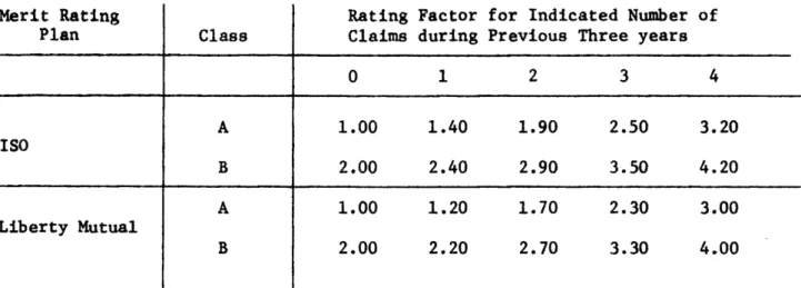
Table 1 presents the incrementalmerit rating factors used in the 1976 rating manuals published by the Insurance Services Office (ISO) and by Liberty Mutual Insurance Company.**

A bivariate model can be used to incorporate both convictions and claims in a manner similiar to that expressed in (5).

This factors differ somewhat by certain secondary rating classes but not by the primary classes reflecting age, sex, etc.

Table 1 Typical Merit Rating Plans

Merit Rating Plan

ISO

Liberty Mutual

Incremental Rating Factors for Indicated Number of Merit Rating Points during previous three years

0 1 2 3 >4 +0.00 +0.00 +0.40 +0.20 +0.90 +0.70 +1.50 +1.30 +2.20 +2.20

13

-If the base premium in a territory for, say, property damage liability was $100, any policy with two merit rating points would pay a $90 surcharge regardless of primary driver class. Both the ISO and Liberty plans apply this incremental

factor in computing premiums for both bodily injury and physical damage cover-age.

The Massachusetts Automobile Rating and Accident Prevention Bureau has provided the author with some preliminary data indicating the fraction of

Massachusetts policies (by coverage) with 0,1,2,... BI, PD or option 1 collision claims during 1975. These data were developed from the experience of a sample of companies writing auto insurance in Massachusetts. An effort was made to count only those claims that would be likely to be considered chargeable acci-dents for the purpose of merit rating under the recently enacted Massachusetts insurance law (Chapter 266 of the Acts of 1976). Table 2 presents some of

together with the

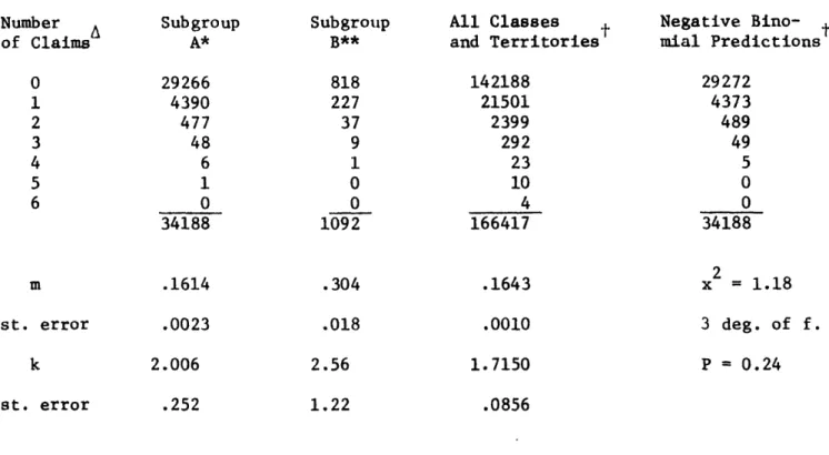
these dat/estimated model parameters for the "no youthful driver" class and one of the youthful driver classes. In both cases an average-risk territory is used. For comparison, the experience for all classes and territories combined is also shown.* Note that the combined experience has a considerably smaller k parameter value indicating--as we expect from the Section 1 discussion--that the distribution of claim likelihood within a class/territory subgroup is con-siderably more concentrated than the aggregate distribution for all policies.

By compounding the estimated gamma-l distribution for claims likelihood given in (3) with the Poisson distribution in (2), one can estimate the fraction of policies within a subgroup characterized by f(rlk,m) who will have 0,1,2,...

In all three cases shown in Table 2, only single-vehicle policies with option 1 collision coverage and voluntary market coverage are considered.

Table 2 Preliminary 1975 Massachusetts Data Number of Claims 0 1 2 3 4 5 6 Subgroup A* 29266 4390 477 48 6 1 0 34188 m .1614 st. error k .0023 2.006 st. error .252 Subgroup B** 818 227 37 9 1 0 0 1092 .304 .018 2.56 1.22 All Classes and Territories 142188 21501 2399 292 23 10 4 166417 .1643 .0010 1.7150 Negative Bino- tt mial Predictions 29272 4373 489 49 5 0 0 34188 2 x = 1.18 3 deg. of f. P = 0.24 .0856

Ahe estimated number of claims.

"at-fault" bodily injury, property damage or collision

A sample of Massachusetts class 10, BI territory 4 policies with a single vehicle, voluntary market coverage, and Bodily Injury, Property Damage, and Option 1

collision coverage.

A similar sample of Massachusetts class 40, BI territory 4 policies. A similar sample of all Massachusetts classes and territories.

- 15

-claims during one year. This compounded distribution is a negative binomial. In Table 2 the predicted negative binomial distribution for the first subgroup is also shown. The good fit is consistent with the results of much more de-tailed tests of the model's accuracy that the author has previously reported using California driver records (Ferreira, 1971). The earlier study used multi-year data and indicated that the predicted posterior distributions for the accident likelihood of drivers with similar records also fit the empirical data well.

4.0 An Illustrative Example

The estimated k and m parameters in Table 2 can be substituted into the merit rating equation given in (5) to examine the indicated premium levels. However the class and territory subgroups considered in Table 2 are only two

of the several dozen currently in use in Massachusetts. In order to obtain base pre-miums needed to develop the applicable ISO and Liberty merit rating prepre-miums

would require much more data than we have provided thus far. To avoid such complications here, we consider instead an illustrative example in which only two clauses and a single territory exist and each class has claims likelihood characteristics similar to the actual subgroups described on Table 2. We shall also assume that each risk class has the same number of policies.

Class A, the low-risk class, has an average claim frequency which we round off to m = 0.15 claims per year while class B has m = 0.30 claims per year. For both classes we assume a shape parameter k = 2.0--close to the estimated value for subgroup A in Table 2 and well within a one standard error range of the estimated value for subgroup B. Figure 3 graphs the predicted percent-age of policies in each class with 0,1,2, and 3 or more claims during a three

F7/g e

3

A

CL

-a a, IS rV?7t L.-O A i 1 sr! 111 B

Class R

B,

Li· , U** . H U N

1

a

CL8..

C

r;iy

70-

Yo0-

30-ut v_U S.

C-, I . r; .,I I.

r-B.: I..

0

B

33

3

,rJ)

I

1

IIIPIIIC -- -,--

fEx p + r

ni e

s9

C

,s.a

17

-year period.*

For clarity, we assume that policies in each class will be priced only on the basis of policy class and the claims experience during the three year period.

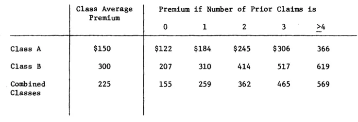
(That is, we have no additional information with which to differentiate among the policies). Also, we ignore differences in the severity distribution for claims in each class and do not explicitly consider the allocation of adjust-ment costs, overhead and the like. Under these conditions, a rating plan based only on the two classes would charge $150 per year to those in Class A and $300 to those in Class B if the average claim cost were $1000.

Figure 4 plots the theoretical distribution of loss potential among

policies in each class. The curves are the gamma-l distributions given in (3) using the appropriate k and m values. Note the extensive amount of overlap. Both distributions are skewed to the right (a property of gamma distributions) and have many policies with a loss potential below the overall average of $225.

Using the mean of the posterior claims likelihood distribution given in (5) we can estimate the average amount of losses during the next year for those policies in each class that had 0,1,2, and 3 or more claims during the last three years.** The estimates are

Class A: Premium = $122 + $ 61 X, and (6)

Class B: Premium = $207 + $103 X, (7)

The predictions are made using the negative binomial distribution mentioned earlier with the selected k and m parameter value for each class.

In making these computations we assume that C. in (5) equals unity so that only the pure premium is considered without loaing for expenses, profit, etc.

/F /a " w e

Zo)J

/o

_16e9 zi Ic

I

6q -LI(~~~~~~~~~~~~~~~~~~~~

a

/00

; 00

300

too

Y400

_t00

'D. . w i4c 191 's -- 4z

- 19

-where X is the number of claims during the previous three years. The coefficients (but not the linear form) of these equations are quite sensitive to the shapes

of the within class loss potential distributions (Figure 2).

The differences between these estimated premiums and the $150 and $300 class averages are the merit rating surcharges and discounts reflecting prior claims experience. In terms of the Bayesian model and a least squares loss function, the estimated premiums are the best we can do in trying to charge policies their expected losses on the basis of class and three years of claims experience. Had the two classes been pooled together before we estimated model parameters, the result would have been m = 0.225, k = 1.51, and merit rating premiums given by

Premium = $155 + $103 X. (8)

Note that these premiums are those that would be estimated if we could obtain claims incidence data (of the type given in Figure 3) only for the combined classes. The three sets of theoretical merit rating premiums are tabulated in Table 3. Table 4 expresses these same premiums in terms of the surcharge or discount relative to the class average premium.

The policies are treated quite differently in each case. The differences are plausible if one focuses on the purpose of merit rating as it was described

in Section 1. Class B policies are expected to have more claims as a group they pay twice as much as Class A but have the same number of policies. Since it is less surprising for a class B policy to have one claim than for a class A policy to have one claim, we expect the class A surcharge for one claim to be higher. The class B policy still pays much more in total premiums, since the one claim is not sufficient to overshadow the two to one claims frequency ratio between the two classes. A class A policy would need three claims in three years before

Tables 3 Theoretical Merit Rating Premiums Class Average Premium $150 300 225

Premium if Number of Prior Claims is 0 $122 207 155 1 $184 310 259 2 $245 414 362 3 $306 517 465

Table 4 Surcharges and Discounts for each Theoretical Plan

Class Average Premium $150 $300 $225 Surcharge or (Discount) Prior Claims is 0 1 ($28) $34

(

93)

(

70)

2

$ 95

10 114 34 137 if the Number of 3 >4 $156 217 240 216 319 344 Class A Class B Combined Classes >4 366 619 569 Class A Class B Combined Classes . .i

21

-the total premium reached -the level charged to a class B policy with one claim during three years.

Alternatively, it is more surprising for a class B policy not to have a claim--and the discount of $93 instead of $28 reflects this.

Finally, class B drivers with several accidents have larger surcharges than class A drivers with the same number of accidents. This situation arises since the class B drivers with the worst records are most likely to be those who in-deed are the highest risks (cf. Figure 4).

The two-class example illustrates how different the implications of having a claim can be for policies in relatively low and high risk classes. The results for the combined risk class case indicate yet one more difficulty. Note from Table 2 that a policy with 2 or more claims pays a larger surcharge under the combined class arrangement than the same policy would under the two-class case. This result occurs because the distribution of expected losses for the combined classes is less concentration than for either of the two classes. When both classification and experiences are considered, the sensitivity of the surcharges to experience is less than when only experience is considered. Upon reflection, this is not surprising, but it can cause problems. If claims incidence data

(such as Figure 3) are obtained for combined classes only and then used to com-pute surcharges to be applied to each risk class, the estimated surcharges will be inappropriate and drivers in the higher risk classes will be overcharged for their accidents. No amount of claims frequency and loss experience data developed from combined classes will point out the inequitable within class distribution of premiums resulting from this error.

Let us now compare these theoretical merit rating premiums with those of typical merit rating plans that surcharge all policies within a territory the

22

-same dollar amount for a specific number of claims. We shall use the ISO and Liberty Mutual plans described earlier. Let the base class be class A policies with 0 claims. Then the class B to class A relativity is 2.00 and the rating

factors to be used for each class/claim count combination are those given Table 5. Using the claims frequency incidences in Figure 3 to estimate the fraction of policies with each rating factor in each class and the assumed 50-50 split between class A and class B, we can compute the estimated average rating factor for each plan. The results are 1.80 for ISO and 1.71 for Liberty when both class relativities and merit rating factors are considered. Dividing the overall premium of $225* by these average factors indicates an ISO base premium of $125 and a Liberty base premium of $131. The resulting merit rating pre-miums are compared with the theoretical rates in Table 6 and Figure 5.

Two basic differences explain the variations between the theoretical and actual rates. First, the ISO and Liberty rating factors increase faster than linearly (recall the theoretical relations in equations (6) and (7) are linear). Secondly, the same rating factors are used for both classes. Although the ratio of average experience between class B and class A is 2 to 1, the ratio of the average theoretical merit rating premiums is only 1.7 to 1. Plans such as the ISO and Liberty will tend to overcharge accident free drivers (especially those in the higher risk classes). If the ISO or Liberty rating factors were

In fact each company would have different loading factors for expenses profit and the like so that territory-wide average premium used by each company would differ.

**

The reason it can be different is that the proportion of people with 0,1,2,... accidents is not the same for each class. If the Figure 2 curves for Class A and Class B had different shapes the ratio of premiums would differ by number of accidents as well.

Table 5 Rating Factors Merit Rating Plan 'ISO Liberty Mutual Class A B A B Rating Claims

Factor for Indicated Number during Previous Three years

of 0 1 2 3 4 1.00 1.40 1.90 2.50 3.20 2.00 2.40 2.90 3.50 4.20 1.00 1.20 1.70 2.30 3.00 2.00 2.20 2.70 3.30 4.00

Table 6 ComparingTheoretical and Typical Premiums

Merit Rating Plan Theory ISO Liberty Theory ISO Liberty Class A B

Premium for Indicated Number of Claims during Previous Three Years

0 1 2 3 4 122 184 245 306 366 125 175 238 313 400 131 157 223 301 393 207 250 263 310 300 288 414 363 354 517 438 432 619 525 524

.·-Qz

K1

KQ - Id -O -C) - o d , d -J 4r, X -- 4 I.

Q

C·t

-'-1

,--r

a - p r `, CC - 1

- o

F-

_Vr

_Kl

-ri

- 0

t~~~

0

~

K % , % O, iCFS , e e , "U U1) 1 Q ct S "t - O 0 -o O 0 mP k -I lip 15 4"C I O .

o

u

m

Qt

0 0 4 M 'd 04"_o I-Ii It i _

~J

S -' r --j -t_{fj 1 o} qj 04 ( r4 QQ \j . C I

(3

q, 1. 'I v

0

,0

25

-changed to 0.00, 0.50, 1.00, 1.50, 2.00, they would better reflect the relations in (6) and (7) for the k 2.0 parameter value situation. Using standard rate-making procedures would then produce class A rates close to the theoretical ones. But the class B rates would be far off with accident-free class B drivers over-charged and Class B drivers with multiple accidents underover-charged.

The graph in Figure 5 highlights this problem. Since the premium differ-entials for both the ISO and Liberty plans are the same for each class, they span a rangethat is too concentrated for class B and too dispersed for class A. In addition the class B premiums begin at too high a level for the claims-free policy.

5. Conclusions and Implementation Issues

In summary, the appropriateness of merit rating depends critically on the distribution of expected losses with each class. Surcharges and discounts developed from aggregate data and applied uniformally across all classes can generate undesirable subsidies.

The results of the paper indicate that certain variations by class in the surcharges and discounts provide a more desirable redistribution of costs than one can obtain using plans currently in use. The author is currently studying a number of related issues (in the context of Massachusetts recent auto insurance

reform law) that must be resolved in order to implement the ideas developed in this paper. Two such issues relate to effects not considered in this paper: (a) how to incorporate convictions for naming violations as well as claims in the merit rating plan, (b) how to estimate and account for the deterrent effect that might arise from introducing merit rating into Massachusetts auto insurance. A third issue is that Massachusetts law provides for surcharges only for

26

-at-fault accidents although the company must pay certain insurance claims re-gardless of fault. Two more issues relate to the nature of auto insurance cover-age: the claims processes for bodily injury, property damage and collision

coverage are not identical and policies with several vehicles must be priced as well. Another issue is the administrative feasibility of implementing such a plan and the possibility of developing plans similar to the ideal one discussed here that enable rapid and accurate determination of premiums by insurance agents. Finally, several credibility and model validity issues must be further developed to determine the extent to which the model applies to Massachusetts experience and the degree of accuracy with which the premiums for a particular

class and territory subgroup can be estimated.

___ _I I IILI 1_1 _ ___ _{._.}

-- 27

References

Arbous, A. and J. Kerrich (1951), "Accident Statistics and the Concept of Accident-Proneness," Biometrics 38, 340-432.

Casualty Actuarial Society (1961), Automobile Insurance Rate Making, New York.

Ferreira, Jr., Joseph (1971), "Some Analytical Aspects of Driver Licencing and Insurance Regulation," MIT Operations Research Center, Technical Report #58, Cambridge, MA.

Ferreira, Jr., Joseph (1974), "The Long-Term Effects of Merit-Rating Plans on Individual Motorists," Operations Research, Vol. 22, No. 5 (September-October 1974).

Seal, H. (1969), Stochastic Theory of a Risk Business, John Wiley and Sons, Inc., New York.