Continuous Multi-Echelon Inventory Optimization by
Sundeep Mathur
Master of Science in Engineering Management, Syracuse University
SUBMITTED TO THE PROGRAM IN SUPPLY CHAIN MANAGEMENT IN PARTIAL FULFILLMENT OF THE REQUIREMENTS FOR THE DEGREE OF
MASTER OF APPLIED SCIENCE IN SUPPLY CHAIN MANAGEMENT AT THE
MASSACHUSETTS INSTITUTE OF TECHNOLOGY May 2020
© 2020 Sundeep Mathur. All rights reserved.
The authors hereby grant to MIT permission to reproduce and to distribute publicly paper and electronic copies of this capstone document in whole or in part in any medium now known or hereafter created.
Signature of Author: ____________________________________________________________________ Department of Supply Chain Management
May 8, 2020
Certified by: __________________________________________________________________________ Dr. Alexis H. Bateman Director, MIT Sustainable Supply Chains Capstone Advisor
Accepted by: __________________________________________________________________________ Prof. Yossi Sheffi Director, Center for Transportation and Logistics Elisha Gray II Professor of Engineering Systems Professor, Civil and Environmental Engineering
Continuous Multi-Echelon Inventory Optimization by
Sundeep Mathur
Submitted to the Program in Supply Chain Management on May 8, 2020, in Partial Fulfillment of the
Requirements for the Degree of Master of Applied Science in Supply Chain Management
ABSTRACT
Global supply chains are becoming increasingly complex systems that drive significant investments in inventory throughout the network. Our sponsor for this project uses a multi-echelon inventory optimization (MEIO) model to manage safety stock inventory across its network. The MEIO model helps them optimize inventory based on upstream and downstream supply chain performance but it does not guarantee year over year reductions in inventory levels that the company desires. To address this issue, we studied how the company can better utilize MEIO to systematically reduce its inventories over time and created a methodology that can be employed by other companies also. We applied the methodology on two products that are presented as case studies. For the chosen products, we found that variation in supply lead time is the primary reason for high MEIO safety stock values. We further identified the underlying cause of variation and provided recommendations to reduce variation in lead time in each case study. This research creates a framework that companies can use to systematically minimize MEIO safety stocks and presents case studies that apply this framework to minimize variation in supply lead time on two products and their corresponding MEIO safety stocks.
Capstone Advisor: Dr. Alexis H. Bateman Title: Director, MIT Sustainable Supply Chains
ACKNOWLEDGMENTS
I would like to thank my adviser, Dr. Alexis H. Bateman, for her mentorship and support throughout this research. Her continuous guidance was invaluable to this project and my learning experience at MIT. I am grateful to staff and faculty at MIT’s Center for Transportation and Logistics for providing us with tools and learning resources that contributed to this project. I especially appreciate the guidance provided by our writing coaches, Toby Gooley and Pamela Siska, who helped refine our message.
I am thankful to the Global Supply Chain leadership team at the sponsor company for allowing us to work on this project and sharing relevant information that made this project a success.
Table of Contents
1. Introduction ... 6
1.1 Problem Definition and Motivation ... 7
1.2 Background: Multi-Echelon Inventory Optimization ... 7
1.3 Research Objective and Scope ... 9
2 Literature Review ... 10
3 Project Methodology ... 11
3.1 Define Phase ... 12
3.2 Measure Phase ... 14
3.3 Analyze Phase ... 16
3.4 Improve and Control Phases ... 19
3.5 Limitations... 19
4 Results ... 20
4.1 Case Study 1: Delays in the start of production order ... 20
4.2 Case Study 2: Variable Production Process ... 25
5 Conclusion ... 29
6 Recommendations ... 32 References
List of Figures
Figure 1: Supply chain network map for MDM Corporation ... 7
Figure 2: Components of the Statistical Safety Stock Model (MEIO) used by MDM Corporation ... 9
Figure 3: Product segmentation by Coefficient of Variation (COV) in Demand and Supply Lead Time ... 14
Figure 4: Analyze Phase: Variation in manufacturing vs shipping lead time ... 18
Figure 5: Analyze phase: Production lead time vs Delay in starting an order ... 18
Figure 6: Case Study 1: Demand and Supply Variability of Product A ... 21
Figure 7: Case Study 1: Variation in manufacturing and shipping lead time ... 23
Figure 8: Case Study 1: Total production lead time vs Days of delay at the start of an order ... 23
Figure 9: Case Study 1: Total production lead time vs Actual time to build an order ... 24
Figure 10: Case Study 2: Demand and Supply Variability for products made at the same facility ... 26
Figure 11:Case Study 2: Variation in manufacturing and shipping lead time ... 27
Figure 12: Case Study 2: Total production lead time vs Days of delay at the start of an order ... 28
Figure 13: Case Study 2: Total production lead time vs Actual time to build an order ... 28
List of Tables Table 1: Data Set 1 for MEIO Calculations ... 15
1. Introduction
Global supply chains are becoming increasingly long and complex networks that drive significant investments in inventory. The service level performance of each tier in such supply chain networks is dependent on the performance of its upstream and downstream tiers. Traditionally, inventory strategies for each tier were set to optimize the performance of that tier that created multiple local optimums and not a global optimum for an end-to-end supply chain. Many companies are now adopting a multi-echelon inventory optimization (MEIO) approach to create global optimums and drive inventory strategy across the network. Adopting MEIO tools to optimize inventory offers improvement in inventory across the network but does not necessarily guarantee a reduction in inventory levels over time that is desired by many companies. This research aims to address this issue by creating a methodology to systematically reduce safety stock inventory for a large healthcare company that utilizes MEIO to set inventory strategy across its network.
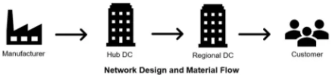
For reasons of confidentiality, we will use MDM Corporation (MDM) as the name for our project sponsor in this paper. MDM Corporation is a Fortune 500 healthcare manufacturer with a product portfolio of over 25,000 stock keeping units (SKU). MDM uses a make-to-stock inventory planning model and builds inventory to forecast and support safety stock requirements in its DC network. Goods are manufactured at MDM’s production facilities and are shipped to a Tier 1 distribution center (DC) which then ships the products to regional DCs. Regional DCs ship products to customers local to that DC (Figure 1). MEIO model is used to calculate safety stock at each of the 40 DCs in MDM’s supply chain network. The company uses a proprietary MEIO software that uses supply variability from upstream tiers, demand variability from downstream tiers, average cycle stock quantity, and service level goals to suggest safety stock inventory targets at each DC.
Figure 1: Supply chain network map for MDM Corporation
1.1 Problem Definition and Motivation
MDM Corporation switched from single-tier optimization to multi-tier inventory optimization software a few years ago. The MEIO software took upstream and downstream DC performance data as input and suggested safety stocks for each DC within their network. Adoption of MEIO led to a large reduction in inventory initially but the safety stock values from the model became stable over time. The company is looking to uncover opportunities to reduce inventories over time. To address this issue, our objective is to create an inventory optimization methodology to systematically reduce inventory levels each year. The methodology will help identify opportunities that will yield the highest savings on inventory carrying costs and recommend ways to improve MEIO safety stocks for those products.
1.2 Background: Multi-Echelon Inventory Optimization
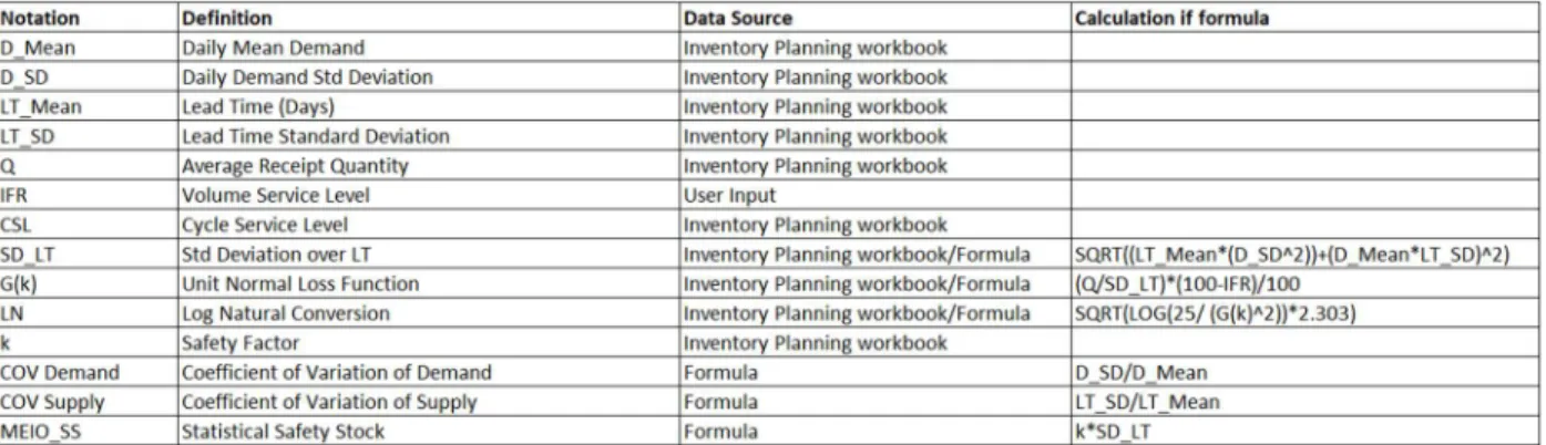
MDM uses a multi-tiered network to manufacture and deliver products to its customers. The company uses a make-to-stock model to build inventory to forecast and place in its Tier 1 distribution center. The inventory policy in these Tier 1 distribution centers is set by the Global Supply Chain Planning group within the company. A proprietary MEIO modeling software is used to calculate safety stocks for all products. The software uses the following data from upstream and downstream supply networks [Figure 2]:
Supply variability, calculated as the standard deviation in lead time over the last six months
We conducted simulations using MDM’s MEIO software and user interviews with the company’s supply chain planners to understand critical inputs to their MEIO model. After analysis, we determined that demand variability is a function of historic sales trends that is outside the company’s control. The demand pattern for such medical devices cannot be shaped by promotions to hospitals. Hence, exploring demand variability to improve safety stocks was ruled out for this project. The second component, average order quantity, is a function of batch sizing in upstream tiers that are outside the scope of this project. Batch sizes are determined by factors other than just inventory carrying cost and changing them did not have a significant impact on MEIO safety stock inventory so it was ruled out for further exploration. The third component, service level target, is set by management and is not considered an input we can change to improve safety stocks in the MEIO model. The fourth and last component, supply variability, is dependent on variability in lead time from upstream tiers of the supply chain and was identified as the primary focus of this project to improve MEIO safety stocks. Supply lead time variability is not actively monitored by the company and many products have consistently high safety stocks because of stable but high variability in supply lead time. For instance, a product may have a Coefficient of Variation (COV) for supply lead time of 60% but because COV is consistently at 60%, MEIO safety stocks for the product remain at the same level (assuming other parameters are constant as well). Reducing COV for such products create a large opportunity for MDM to systematically reduce inventories. We will focus the capstone on reducing this variation in supply lead time for MDM.
Figure 2: Components of the Statistical Safety Stock Model (MEIO) used by MDM Corporation
1.3 Research Objective and Scope
The objective of this research is to create an inventory optimization methodology to systematically reduce inventory levels each year. The methodology will help identify opportunities that will yield the highest savings on inventory carrying costs and recommend ways to improve MEIO safety stocks for those products. This process can be adopted in other companies that utilize MEIO to set inventory levels in their supply chain network.
The paper is structured as follows. In Section 2, we provide a literature review about inventory optimization strategies and MEIO specifically. In Section 3, we present the methodology used to create the framework. In Section 4, we apply the framework on two products and present them as case studies. Section 5 provides a conclusion and Section 6 provides recommendations to MDM Corporation that can be applied by other companies utilizing the MEIO model to set their safety stock policies.
2 Literature Review
MEIO safety stock model has been a topic of study since the 1950s and has been extensively documented especially after the 2000s (de Kok, Ton & Grob, Christopher & Laumanns, Marco & Minner, Stefan & Rambau, Jörg & Schade, Konrad, 2018). The majority of research in this area has been done to create optimal policies to reduce costs. These studies mainly focus on the selection of the right inventory policy for a certain situation to optimize inventory levels. With the improvement in technology, many companies started finding applications of this research in multi-echelon supply chain networks to reduce inventory costs and to create more dynamic inventory policies. These policies used data from upstream and downstream nodes in the supply chain to optimize inventory levels throughout the network. This also led to the development of software to optimize inventory levels. MDM Corporation uses similar software to set inventory policies.
Other studies related to multi-echelon optimization focus on approaches to simulate and measure the performance of a network when a specific policy is selected. For example, Eddoug, ElHaq, and Echcheikh (2018) constructed a simulation to measure the impact of various inventory policies on service level and total cost but their objective is to pick the best model and not to improve inventory recommendations from the same model over a period. Such studies are useful to understand the impact of switching to the MEIO safety stock model but do not suggest ways to improve safety stocks from the same MEIO model.
The impact of variability on inventory performance has also been documented. This relates to the hypothesis of this capstone that improving supply variability will reduce inventory levels. For instance, Wright (2019), documents the impact of demand variation and the bullwhip effect on inventory performance of a pharmaceutical supply chain. The impact of variability in the supply chain has been
quantified in other studies in various supply chain industries as well (Castilho, Lang, Peterson, Volovoi, 2015). However, the impact of supply lead time variability on MEIO and the creation of a methodology to systematically improve inventory performance has not been documented. Our goal is to help MDM Corporation reduce their inventory and document this framework so it can be utilized by other companies and researchers for further exploration of this topic. We will also provide case studies that will document real-world examples to reduce supply lead time variability.
In conclusion, documented research focuses on choosing the right inventory policy or simulating the impact of demand or supply variation on costs. This capstone examines the importance of reducing supply lead time variation to reduce MEIO safety stocks and create a framework that can be used by companies to reduce inventory over time.
3 Project Methodology
The objective of this research is to create a framework to reduce supply lead time variability in supply chain for a large portfolio of products. In this section, we present the methodology used by the project team to reduce this variability. We will use this methodology on two products to show how this can be generalized and applied by other companies.
To create the framework, we adopted Six Sigma’s DMAIC (Define, Measure, Analyze, Improve, Control) approach to define the scope and analyze improvement opportunities in this capstone (Mast, J.D., & Lokkerbol, J.,2012). Each phase in DMAIC has multiple steps of quantitative analysis and deliverables within it. We provide a detailed explanation of each phase in this section.
Here is a summary of each phase in the DMAIC cycle to help create a continuous inventory optimization program for the company:
• Define Scope and Impact of Variation: Segment products with high safety stock inventory cost, high coefficient of variation of supply, low coefficient of variation of demand; Select products that meet the criteria for next step
• Measure and Collect Data: Collect data for all input parameters for MEIO along with corresponding MEIO values
• Analyze Data for Sources of Variation: Identify the root source that causes supply lead time variation for the selected product
• Improve Root Cause: Collaborate with manufacturing, logistics, DC operations or other relevant function to eliminate the source of variation
• Control: Create metrics to monitor progress
This capstone will cover the Define, Measure, and Analyze phase of this project. We will provide high-level recommendations for Improve and Control phases but they will not be covered in this capstone, as their implementation requires additional time and internal company resources for implementation. The following sections explain each phase in detail.
3.1 Define Phase
Multi-billion dollar companies generally have a large portfolio of products that make it difficult to focus on all products for any project. MDM Corporation also has a wide portfolio of products with more than 25,000 finished items for inventory management. The goal of this phase is to identify target products to improve supply lead time variability that will deliver significant cost improvements to the company. In the
case of this capstone, this phase was applied to a business unit with 60 product families that consisted of 550 items or SKUs.
3.1.1 Process Steps
The following process steps were followed to segment product families and select the most impactful products.
I. Filter products with safety stock value greater than $10,000
II. Segment products by the coefficient of variation of demand and supply III. Shortlist products with the highest supply variation and high inventory costs
IV. Conduct internal stakeholder discussion to select target products for next phase of DMAIC cycle
As a final deliverable for this phase, products that meet the criteria specified were identified for further exploration. Shortlisted products were reviewed with project sponsors and two products (Product A and Product B) were selected for this pilot project based on the strategic importance and impact on cost savings to the company.
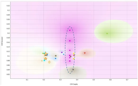
Figure 3 shows products by coefficient of variation of demand (COV Demand) on the vertical axis and coefficient of variation of supply lead time (COV Supply) on the horizontal axis for products. All products on the graph have safety stock value greater than $10,000. Based on internal stakeholder discussion, Product A and Product B were chosen as pilot products for further analysis of supply variation. Specific details for each product are provided in case studies in Section 4 of this paper.
Figure 3: Product segmentation by Coefficient of Variation (COV) in Demand and Supply Lead Time
The figure shows Product A, marked by symbol x, has 6 individual finished parts that have a high coefficient of variation of supply and is a good candidate for the next phase.
3.2 Measure Phase
The purpose of this phase is to collect and aggregate data sets for the analysis phase. MDM Corporation uses proprietary software for MEIO model calculations and all the data resides in their system. We used the data available in their software as the source for this capstone. The data used was for the year 2019 and included MEIO suggestion by-product, corresponding demand, lead time, service level target, and average order quantity detail. Once the data is collected, it is compiled at the part level into two data sets.
3.2.1 Data Set 1 for MEIO Calculations:
This data set was used to understand the impact of variation on the pilot products and to verify the hypothesis that high variation in supply is the primary reason for higher safety stocks. The primary features of this data set are the Coefficient of Variation of supply, coefficient of variation
of demand, average receipt quantity, and item fill rate target (or volume service level). See Figure 2 for graphical representation and Table 1 for a detailed field list of this data set.
3.2.2 Data Set 2 for Supply Variation Analysis:
This data set was used to progressively analyze the root cause of the supply variation. This data set breaks down supply variation into variation due to the manufacturing site and due to the shipping process. The manufacturing site variation is further broken down into variation in lead time due to planner overriding system suggested order start date and variation in lead time due to the manufacturing process. There could be multiple reasons for planners to override the system suggested start date for an order. The most common are component shortages and changes in production line capacity due to operator shortages. Variation in the manufacturing process occurs if the process is not well-controlled and it may take different time to build the same number of units of the same product from one order to the other. See Figure 2 for graphical representation and Table 2 for a detailed field list of this data set.
Table 2: Data Set 2 for Supply Variation Analysis
Data for the capstone was collected in September 2019 from several reports within the company and aggregated using MS Access. It is important to note that the data was collected for the same time interval across this analysis. Aggregated data was fed into the next phase of analysis using a visualization software like Orange. The final deliverable for the measure phase is two data sets as stated above for the project sponsor. The data schema might differ when the project is reproduced for other companies, but primary data features are expected to be the same for most safety stock models.
3.3 Analyze Phase
The primary focus of this phase is to understand the sources of variation in supply for selected products. We followed an iterative approach to understand the root cause of variation that MDM needs to fix to reduce safety stocks. We break down supply variation into manufacturing variability and shipping lead time variability and analyze factors that most significantly cause process variation. Figure 2 describes how supply variability from the start of order in manufacturing to delivery in a Tier 1 DC is broken down into smaller components for this analysis.
3.3.1 Process Steps
The section below describes an iterative methodology to identify the source of variation in supply. These steps are specific to MDM Corporation based on the setup of their supply chain systems
but at a macro level, the approach will be similar for other companies using different supply chain systems.
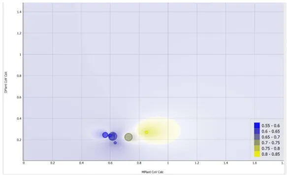
I. Root-cause Level 1: Shipping lead time versus manufacturing lead time variability
The objective of this step is to understand the primary driver of supply variability by analyzing variability in shipping (CoV DPlant) and variability in the manufacturing process (CoV Mplant). See Figure 4.
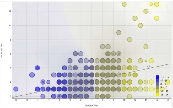
II. Root-cause Level 2: Breaking down Level 1
The objective of this step is to break down the components of shipping lead time or manufacturing lead time variability and investigate the data further. For instance, we analyzed the drivers of variability in the manufacturing process (CoV MPlant) for Product A. We found that there are two primary drivers, variability in system suggested and actual start dates for an order due to a system override entered by materials planner (termed Delayed Start) or lead time variability in the manufacturing process. Figure 5 breaks down the total lead time into delayed starts and actual lead time in manufacturing. Delayed start lead time (in days) represents if the order was started early or late compared to the system suggested date for the origination of the order. Actual lead time represents the lead time for the physical production of an order. Each dot represents a single order from Jan - Sep 2019.
III. Root-cause further analysis
Progressively break down the sources until the root cause for supply variation is determined. In this case, the root cause was identified at the previous level and no further analysis was needed.
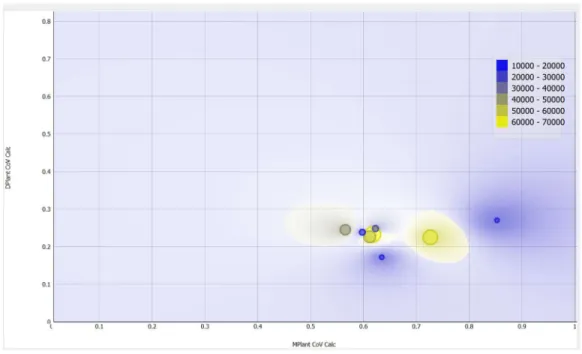
Figure 4: Analyze Phase: Variation in manufacturing vs shipping lead time
Manufacturing Variability (MPlant CoV) v/s Shipping Variability (DPlant CoV) for Product A. Figure shows that MPlant CoV is much higher than DPlant CoV. Hence, MPlant CoV should be analyzed further.
Figure 5: Analyze phase: Production lead time vs Delay in starting an order
Lead time from system suggested start date for a production order to actual release for shipping to DC is broken into Delayed Start (X-axis) and Actual Production Lead Time (Y-axis).
The root cause of supply lead time variation is determined at the end of this step. The next phase of the project is to implement and monitor the improvements. The MEIO model will pick up the improvements over time as history builds up in its input data and will lower safety stocks as a result.
3.4 Improve and Control Phases
As the next step, we recommend MDM Corporation’s production and distribution teams to brainstorm solutions to alleviate root causes of variation identified in the Analyze phase. Once a fix has been identified and implemented, the variation in supply lead time is expected to diminish. The reduction in supply lead-time variation will be recorded by the MEIO model over lead-time and will result in the reduction of the safety stocks for downstream DC. The Improve and Control Phases are outside of the scope of this capstone as they require teams internal to MDM Corporation that we do not have access to and require a longer time horizon to implement and monitor the process.
3.5 Limitations
The Improve and Control Phases are outside of the scope of this capstone as they require teams internal to MDM Corporation that we do not have access to and require a longer time horizon to implement and monitor the process. Also, we applied this methodology to a set of products from one division of MDM Corporation that are make-to-stock and strictly follow the MEIO safety stock model. Our methodology is most suited to such products and may need to be adapted for companies with different supply chain models. We also used historical data in our analysis and our results for the same products may change if the conditions in manufacturing and distribution change. For instance, a long-term component shortage may hamper a production line’s ability to meet schedule and increase variability. Our analysis may not be
4 Results
The goal of this project is to devise a methodology for MDM Corporation to continuously lower its inventory investment throughout its supply chain network. This project adopts Six Sigma DMAIC cycle to create such a continuous inventory optimization program. The methodology lays out various steps to define the scope, measure variation, and analyze primary sources of variation in the supply chain for the MDM Corporation.
We present the results in the form of two case studies to demonstrate the results of applying this methodology at MDM Corporation. Two different products with different primary sources of supply lead time variability are chosen for the case study. The case studies will present the results of steps to the Define and Analyze phase as described in Section 3. Steps in Measure phase are for data collection and are not part of the result. Also, as stated earlier, the Improve and Control phases are outside the scope of this capstone due to time limitations to time limitations to complete the project.
4.1 Case Study 1: Delays in the start of production order
The first product is chosen (Product A) is manufactured at a facility in Indiana, USA. The product has a stable demand but a highly variable supply. High variation in supply leads to a disproportionate increase in safety stock when compared to other products manufactured at the same manufacturing facility. The case study will explore the root cause of this issue.
4.1.1 Define Phase:
The objective of this phase is to select relevant products for analysis. The company is looking to lower the investment in inventory while maintaining service levels, hence products with
large inventory investments are used as the first criteria for selection. In this case, products families with more than $10,000 in safety stock investment value are selected.
The next level of criteria is to identify products with large variations in demand or supply lead time. As discussed above, the demand pattern for products sold by MDM Corporation cannot be impacted hence we focus on products with a high coefficient of supply (CoV Supply). Comparing CoV of Supply for various products manufactured by the company, it was determined that products with CoV Supply greater than 30% are considered highly variable. Thus, our goal is to identify families with high inventory investment and high CoV Supply. Figure 6 identifies Product A as a candidate for further analysis.
Figure 6: Case Study 1: Demand and Supply Variability of Product A
4.1.2 Analyze Phase
The objective of this phase is to understand the primary source of variation in supply lead time. As detailed in section 3.3.1, the source of variation is understood by applying a top-down approach to decipher the root-cause.
We will analyze the coefficient of variation of lead time for shipping and the coefficient of variation of lead time for manufacturing the same product for data collected over six months in 2019 (Figure 7). This comparison will help us understand which of the two factors is dominant and must be explored further to identify the root cause. It is evident from the figure that variation in manufacturing lead time is much larger than variation in shipping lead time. Hence, we explore the reasons for variation in manufacturing lead time.
Manufacturing lead time can be broken into delayed start (time between system suggested start of production order and actual start) and lead time from the actual start of the production order to when it is finished). After analyzing the data, it was determined that for Product A, the delayed start is highly variable for each production order of Product A and is the most dominant factor that contributes to increased total lead time. Figure 8 shows a highly deviant delayed start from -4 days (early start) to + 10 days (order started 10 days later than system suggestion) and a strong correlation between the two axes. After reviewing the results from Figure 9, the delayed start was considered as the primary source of variation in supply lead time.
Figure 7: Case Study 1: Variation in manufacturing and shipping lead time
Variation in Lead time in Manufacturing (MPlant CoV) versus Variation in Lead time in Shipping (DPlant CoV). The figure shows that the lead time in manufacturing is a highly variable process.
Figure 9: Case Study 1: Total production lead time vs Actual time to build an order
The figure shows a weaker correlation between the two axes, hence actual lead time was ruled out as the primary cause of variation in supply lead time.
4.1.3 Case Study 1 Conclusion
From the results described above, the delayed start of a production order compared to the system suggestion was confirmed as the primary source that causes a variable supply lead time. After speaking with production teams at the manufacturing site, it was discovered that the materials planners often manually intervened and updated the planning system with a different start date for production orders based on the availability of a sub-component. The planning of sub-components is managed outside the software used for finished goods by the company, hence, the component level changes in supply are not factored in start production orders. To avoid operators to be idle due to a lack of components, the manufacturing planners frequently override production start dates for finished goods. This process introduces variability in the total lead time of a production order. Our objective will now be to improve this source of variability.
The production teams identified that Kanban’s and safety stock settings for the sub-component were out of date compared to current demand. The Improve phase is out of the scope of this capstone, however, the teams will be focusing on updating safety stock settings for the sub-components to improve overall supply variability.
4.2 Case Study 2: Variable Production Process
The second product chosen (Product B) is manufactured at a facility in Costa Rica. The product has a stable demand but a high manufacturing lead time. High variation in supply leads to a disproportionate increase in safety stock when compared to other products manufactured at the same manufacturing facility. The case study will explore the root cause of this issue.
4.2.1 Define Phase:
As described in the previous case study, the objective of this phase is to select relevant products for analysis. We have chosen product B because the inventory investment for this product is greater than $10,000.
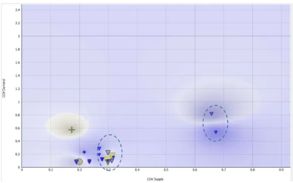
The next level of criteria is to identify products with large variations in demand or supply lead time. As discussed above, the demand pattern for products sold by MDM Corporation cannot be impacted hence we focus on products with a high coefficient of supply (CoV Supply). Comparing CoV of Supply for various products manufactured by the company, it was determined that products with CoV Supply greater than 30% are considered highly variable.
Figure 10: Case Study 2: Demand and Supply Variability for products made at the same facility The figure shows Product B, marked by a symbol triangle, has many individual finished parts that have a high
coefficient of variation of supply and is a good candidate for the next phase.
4.2.2 Analyze Phase
The objective of this phase is to understand the primary source of variation in supply lead time. As detailed in section 3.3.1, the source of variation is understood by applying a top-down approach to decipher the root-cause.
Figure 11 describes the coefficient of variation of lead time for shipping versus the coefficient of variation of lead time for manufacturing the same product for data collected over six months in 2019. It is evident from the figure that variation in manufacturing lead time is much larger than variation in shipping lead time. Hence, we explore the reasons for variation in manufacturing lead time.
Manufacturing lead time can be broken into delayed start (time between system suggested start of production order and actual start) and lead time from the actual start of the production order to when it is finished). After analyzing the data, it was determined that for Product B, manufacturing lead time is highly variable for each production order of Product B and is the most dominant factor that contributes to increased total lead time. See Figures 12 and 13 for further explanation of results.
Figure 11:Case Study 2: Variation in manufacturing and shipping lead time
Variation in Lead time in Manufacturing (MPlant CoV) versus Variation in Lead time in Shipping (DPlant CoV). The figure shows that the lead time in manufacturing is a highly variable process compared to shipping lead time.
Figure 12: Case Study 2: Total production lead time vs Days of delay at the start of an order
The figure shows a highly deviant total lead time but not the delayed start time. The correlation between the two axes is not strong so delayed start is ruled out as the primary source of lead time variation.
Figure 13: Case Study 2: Total production lead time vs Actual time to build an order
The figure shows a strong correlation between the two axes, hence actual lead time is considered as the primary cause of variation in supply lead time.
4.2.3 Case Study 2 Conclusion
From the results described above, the actual lead time of a production order has been verified as the primary source that causes a variable supply lead time. Our objective will now be to improve this source of variability.
After speaking with production teams at the manufacturing site at the MDM Corporation, it was discovered that this production line has many steps and is used to manufacture more than 200 items that belong to the same family of products. It was determined that work in process (WIP) inventory should be pulled by operators on the production line based on first in first out (FIFO) process. However, operators give priority to high volume items which cause some lower-volume items to remain in WIP for a longer period. This introduces variability in the system and raises the standard deviation of manufacturing lead time for the entire product family, thereby raising the value of safety stock inventory needed in Tier 1 distribution centers.
The improve phase is out of the scope of this capstone, however, the teams will be focusing on implementing robust processes, so all products are in WIP are given equal priority. The priority should be determined by the system before beginning a production order, however, once the order has been started all WIP steps should execute based on the FIFO process.
5 Conclusion
create a supply chain strategy. We started by understanding the key components of this model, which were demand variability, supply variability, average order quantity and service level target.
First, we concluded that demand variability in the MEIO model is outside the control of the company. The company manufactures and sells medical devices and demand is dependent on the rate of surgeries in hospitals which cannot be shaped. This led us to focus on supply variability as the most dominant factor leading to an increase in the company’s safety stock.
Second, we adopted Six Sigma’s DMAIC methodology to scope, measure and analyze products with high supply variability. We analyzed a large portfolio of products and used the methodology to identify two products with high safety stock investment and high supply variability. We analyzed the source of variability for each product in further detail and identified the root cause of variation in supply lead time for the company to improve.
For Product A manufacturing in the US, we concluded that the shipping lead times are stable, but manufacturing lead times are variable. Investigating further, we found that lead time to manufacture order is stable, but the orders do not always start on time. The delayed start of orders was due to manufacturing planners' overriding system-suggested start dates based on factors like component or labor availability. These factors are not captured in the MEIO system used at the company. Our recommendation to the company for this product was to review component safety stock levels and ideally use the MEIO model to drive their supply.
For Product B manufactured in Costa Rica, we noted that the shipping lead times are stable but the manufacturing lead times are variable. In this case, however, we found that the manufacturing process
was not under control and an order for the same product took anywhere from 20 to 60 days to build. After working with the production planning team in Costa Rica, we found that this production line involves many sub-processes and that the standard lead time to manufacture a product is 2 weeks. Product B had a very high number of SKUs, and operators picked the highest volume SKUs to work on their station as they understood those products are strategic. This resulted in increased wait time between stations and an increased total production time for low volume SKUs and very less wait time between stations and standard total production time for high volume SKUs. This however led to a highly degree of variation in lead time from one order to the other on the production line. We recommended to strictly enforce first-in, first-out (FIFO) process at each step of manufacturing on this product line as operators should not pick which order to work on next. Rather, operators should follow the queue established by the planning system that considers other factors to determine order priority.
By using the framework on the two pilot products above, we intended to show how companies can systematically improve supply variability and lower their inventories over time. We recommend that a central group within a company should manage the process to define the scope and work with respective local teams to implement solutions.
In addition to the framework, we attempt to shift the dialogue from benefits of MEIO implementation and using it as a black box to deeper understanding of how the MEIO model calculates safety stocks for a company. Implementing MEIO can result is a step reduction in inventory values for a company but understanding how MEIO drives inventory in the network will help them identify future improvements opportunities.
6 Recommendations
Most companies utilize MEIO model to set safety stocks in their network. However, given the same demand and service requirements for a product, the output of MEIO model output will remain the same. MDM Corporation is looking to reduce their inventory levels and we recommend a methodology in this paper to lower safety stocks over time. This approach will help MDM identify products to target for reduction and identify actions needed to reduce safety stocks. We identified ways to supply lead time variability for products in scope of this project. The methodology used can be expanded beyond MDM Corporation and adapted by other companies to improve their safety stock inventory levels.
Additionally, we recommend the methodology to be implemented by a central team at MDM Corporation. Managing centrally will ensure fulfillment of end-to-end supply chain goals and global optimization of supply chain rather than by site. It would be helpful to develop metrics to detect trends in variation before they start impacting MEIO safety stocks that use 6 months historical data as input. This will ensure fixing the problems before an investment in inventory is made by the company. This work can be extended by applying the methodology to improve demand variability.
References
de Kok, T. & Grob, C. & Laumanns, M. & Minner, S. & Rambau, J. & Schade, K. (2018). A typology and literature review on stochastic multi-echelon inventory models. European Journal of Operational Research. 269. 10.1016/j.ejor.2018.02.047.
Eddoug, K., ElHaq, S. L. & Echcheikh, H. (2018). Performance evaluation of complex multi-echelon distribution supply chain, 2018 4th International Conference on Logistics Operations Management (GOL), Le Havre, 2018, pp. 1-10.
Castilho, J., Lang, T., Peterson, D., and Volovoi, V. (2015). Quantifying variability impacts upon supply chain performance. In Proceedings of the 2015 Winter Simulation Conference (WSC ’15). IEEE Press, 1892–1903.
Wright, M. (2019). An Analysis and Mitigation of Demand Variability on External Supply Chains. Thesis, Massachusetts Institute of Technology, 2019. https://dspace.mit.edu/handle/1721.1/122267. Schneider, C. (2016). Modeling End-to-End Order Cycle-Time Variability to Improve on-Time Delivery
Commitments and Drive Future State Metrics. Thesis, Massachusetts Institute of Technology, 2016. https://dspace.mit.edu/handle/1721.1/104390.
Mast, J.D., & Lokkerbol, J. (2012). An analysis of the Six Sigma DMAIC method from the perspective of problem solving.