Lattice-based and topological representations of binary relations with an application to music

HAL Id: hal-01256854

https://hal.archives-ouvertes.fr/hal-01256854

HAL is a multi-disciplinary open access archive for the deposit and dissemination of sci-entific research documents, whether they are pub-lished or not. The documents may come from teaching and research institutions in France or abroad, or from public or private research centers.

L’archive ouverte pluridisciplinaire HAL, est destinée au dépôt et à la diffusion de documents scientifiques de niveau recherche, publiés ou non, émanant des établissements d’enseignement et de recherche français ou étrangers, des laboratoires publics ou privés.

Lattice-based and topological representations of binary

relations with an application to music

Anton Freund, Moreno Andreatta, Jean-Louis Giavitto

To cite this version:

Anton Freund, Moreno Andreatta, Jean-Louis Giavitto. Lattice-based and topological representations of binary relations with an application to music. Annals of Mathematics and Artificial Intelligence, Springer Verlag, 2015, 73 (3-4), pp.311-334. �10.1007/s10472-014-9445-3�. �hal-01256854�

Lattice-based and Topological Representations of Binary

Relations with an Application to Music

Anton Freund

Ludwig–Maximilians–Universit¨at, Munich, Germany afreund@phare.normalesup.org

Moreno Andreatta

CNRS – UMR 9912, IRCAM & Sorbonne Universit´es–UPMC, France Moreno.Andreatta@ircam.fr

Jean-Louis Giavitto

CNRS – UMR 9912, IRCAM & INRIA Rocquencourt MuTAnt team & Sorbonne Universit´es–UPMC, France

Jean-Louis.Giavitto@ircam.fr

Abstract

Formal concept analysis associates a lattice of formal concepts to a binary relation. The structure of the relation can then be described in terms of lattice theory. On the other hand Q-analysis associates a simplicial complex to a binary relation and studies its properties using topological methods. This paper investigates which mathematical invariants studied in one approach can be captured in the other. Our main result is that all homotopy invariant properties of the simplicial complex can be recovered from the structure of the concept lattice. This not only clarifies the relationships between two frameworks widely used in symbolic data analysis but also offers an effective new method to establish homotopy equivalence in the context of Q-analysis. As a musical application, we will investigate Olivier Messiaen’s modes of limited transposition. We will use our theoretical result to show that the simplicial complex associated to a maximal mode with m transpositions is homotopy equivalent to the (m − 2)–dimensional sphere.

Keywords. formal concept analysis; Q-analysis; simplicial complex; homotopy invariance; Betti numbers; combinatorial classification of harmonies; mode of lim-ited transposition

1

Introduction

Formal concept analysis (FCA) relies on lattice theory for the analysis of binary relations. It has been developed around 1980 by Rudolph Wille [Wil82], Marc Barbut, Bernard Monjardet [BM70] and others. Another approach to the analysis of binary relations is to give them a topological representation in terms of a simplicial complex. Originating in Dowker’s research on the homology groups of relations [Dow52], this idea has been developed by Ronald Atkin under the name of Q-analysis1 _{since the beginning of the 1970s [Atk72] and has been applied}

to many problems in the social sciences [Cas79, Fre80, Joh91, DN97, BKLW01].

Both frameworks heavily rely on lattice theory, an enabling instrument for rigorous anal-ysis and design in AI [Kab11]. Both focus on the backcloth representation of binary relations

1

This methodology is not to be confused with an algorithm that groups objects (from variables) and is called Q-analysis or Q-factor analysis (in opposition to R-analysis that groups variables).

relating two sets of indicators, features or characteristics. They both have been developed for and applied to the qualitative analysis of symbolic data where they have proven espe-cially useful in solving problems involving systems with complex structures. They provide respectively algebraic and topological tools for data reduction that facilitate an agnostic and macroscopic conceptualization of the systems. Yet, it does not exist a thorough comparison of these two theoretical approaches.

Contributions. The aim of this article is to compare the two approaches from a mathe-matical point of view: A first observation will be that each approach captures information which is neglected in the other. To see this we will exhibit different relations which give rise to equal (more precisely: isomorphic) concept lattices but to different (non-isomorphic) simplicial complexes, and vice versa. This means that neither the concept lattice nor the simplicial complex can in general be fully reconstructed from the other object.

In contrast to this negative result we will show that (the isomorphism class of) the concept lattice alone allows to determine the homotopy type of the simplicial complex, i.e. most properties typically studied in the topological approach. Sections 2 to 6 of the present paper are devoted to these theoretic questions.

This result is of fundamental interest: it relates two approaches in the analysis of a binary relation, an order theoretic one and a topological one. It has also a practical interest because some topological questions are more simple to answer in the framework of lattice theory and vice versa. We show an application in the field of mathematical music theory in section 8: We use the results of the previous sections to investigate simplicial complexes associated to modes of limited transposition. This is inspired by Michael Catanzaro’s [Cat11] classification of the simplicial complexes associated to prime forms with three chromas.

2

A brief tour in FCA and Q-analysis

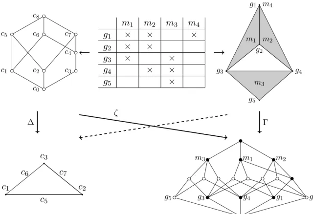
Both FCA and Q-analysis study the relationships between two finite sets by looking at the boolean matrix specifying the interactions between elements of the sets. Following the ter-minology of formal concept analysis we associate rows of this incidence matrix with objects and columns with attributes. Then the table contains the value true at position (i, j) if the i-th object has the j-th attribute. See figure 1 (top center) for an example (crosses represent the value true).

2.1 FCA background

The formal notion corresponding to such a table is that of a formal context. We will often drop the specification “formal”.

Definition 2.1. A formal context2 is a triple K = (G, M, I) where I ⊂ G × M is a binary relation. Elements of G are called objects and elements of M are called attributes. We always assume that G and M are finite, and that the formal context is clarified. The latter means that no object has all attributes and that no attribute holds for all objects.

The requirement of finiteness and the interdiction of full rows and columns is usually not included in the definition. As shown in [GW99, p. 27] the latter is not actually a restriction

2

from the perspective of formal concept analysis. Finiteness is given in most applications. The reasons for this restriction will be seen in the sequel.

Such a context can be analysed using the methods of formal concept analysis. The central notion is that of a (formal) concept. To get some intuition, let us consider the context in the upper middle of figure 1. Following an example of Atkin [Atk78], one can imagine that the five objects g1, . . . , g5 represent five people working on a joint project. To coordinate their

work they have established four regular meetings m1, . . . , m4, each with different participants.

There is a cross at position (i, j) if the i-th person is a member of the j-th meeting group. How can we find reasonable organisational substructures of that collaboration? Let us think about people first: Do person 1 and person 3 constitute an interesting subgroup? An answer in the spirit of formal concept analysis is no: The only meeting at which both of them participate is m1. However m1 has an additional participant, namely person g2. So if we are

looking for an organisational group containing g1 and g3, then we should also include g2, who

is present at all their joint meetings.

We can also think the other way around: Do meeting m1 and m2 form an interesting

collection of meetings? Our answer is yes: The only people who are participating at both of these meetings are g1 and g2. Furthermore m1 and m2 are the only meetings which these two

people share. So this seems to be their forum.

Generalizing the example, a formal concept is a pair consisting of a set of objects and a set of attributes of a formal context. The two sets have to be maximal in the sense that there are no other objects having all attributes in the list and no other attributes that hold for all the objects. As before we drop the specification “formal” when talking about formal concepts.

Definition 2.2. Let K = (G, M, I) be a context. For sets A ⊂ G and B ⊂ M we define associated sets A0⊂ M and B0 ⊂ G as

A0 := {m ∈ M | (g, m) ∈ I for all g ∈ A} and B0 := {g ∈ G | (g, m) ∈ I for all m ∈ B}.

A pair (A, B) of sets A ⊂ G and B ⊂ M is called a formal concept if we have A0 = B and B0= A. The set A is called the extent of the concept and the set B is called its intent.

As shown in [GW99, p. 19] the prime operators in the two directions induce a Galois connection. We will not need this notion in general but shall eventually invoke certain facts that it implies. We can order concepts according to set-theoretic inclusion of their extents, making one concept bigger than another if it includes all objets falling under the competitor, and more. It is proved in [GW99, p. 20] that the resulting order is a lattice. Staying in the above example a meeting is termed bigger — or superordinate — compared with another if it has at least all the participants of the smaller meeting. Figure 1 (top left) depicts the whole concept lattice of the example.

Definition 2.3. Let K be a context. We define an ordering ≤ on its concepts by putting (A, B) ≤ (C, D) if and only if A ⊂ C,

for two concepts (A, B) and (C, D). The resulting order is called the concept lattice of K and is denoted by B_K.

c8 c5 c6 c7 c4 c1 c2 c3 c0

m

m

m

m

g

×

×

×

g

×

×

g

×

×

g

×

×

g

×

ζ

c

c

c

c

c

c

Figure 1: In the upper part of the diagram one finds a formal context (center), the associated concept lattice (left) and the associated simplicial complex (right). The formal concepts of the concept lattice are given as c0 = (∅, {m1, . . . , m4}), c1 =

({g3}, {m1, m3}), c2 = ({g4}, {m2, m3}), c3 = ({g1}, {m1, m2, m4}), c4= ({g1, g2}, {m1, m2}),

c5 = ({g3, g4, g5}, {m3}), c6 = ({g1, g2, g3}, {m1}), c7 = ({g1, g2, g4}, {m2}) and c8 =

({g1, . . . , g5}, ∅). In the simplicial complex filled triangles correspond to 2-dimensional

sim-plices while the triangle in the middle is a hole. The lower part of the diagram, in particular the meaning of ∆, Γ, ζ and the dashed arrow, is explained in Section 3.

Invoking definition 2.2 it is straightforward to show that (A, B) ≤ (C, D) as defined is equivalent to B ⊃ D. Note that our definition of context implies that (∅, M ) and (G, ∅) are always concepts. They are the least and the greatest element of the lattice.

We are mostly interested in properties of the concept lattice which do not depend on the labelling but only on the form of the lattice. Formally these are properties which are preserved under isomorphisms of partial orders. An example of such a property is the number of atoms (upper neighbours of the least element) of the lattice.

2.2 Q-analysis background

Another way to represent a table for data analysis is in the form of a simplicial complex. Such a complex represents a generalized polyhedron in a suitable multidimensional Euclidian space whose vertices are the objects (the rows) or alternatively the attributes (the columns) of the table.

vertices which may be pictured as the target points of linearly independent vectors in some Euclidian space. The simplex is then the convex hull of its vertex set. For instance, a simplex with three vertices is a triangle and a simplex with four vertices is a tetrahedron. By glueing such simplices along their vertices, edges and higher-dimensional sub-simplices we obtain what is called a simplicial complex. We could glue for example three line segments to form the boundary of a triangle, with the interior of the triangle left empty.

Typical topological questions about a simplicial complex are: Is it connected? i.e. can we find a path from any point of the simplicial complex to any other without leaving it? For the boundary of a triangle this is the case. Is it simply connected? i.e. can every closed curve on the simplicial complex be contracted to a single point, or are there “holes” in the simplicial complex which prevent this? For example a filled triangle is simply connected, but the boundary of a triangle is not, since a curve which goes around once cannot be contracted without “jumping” over the hole in the middle.

For our investigation it will often be useful to abstract from the geometric nature of a simplicial complex: We do not mind which precise shape the boundary of a triangle has, as long as it consists of three vertices which are pairwise connected but do not all three belong to one common simplex. For more detailed explanations of topological notions we refer to [Hat02, chap. 1]. Discarding the geometrical interpretation of simplicial complexes we get the following definition.

Definition 2.4. An abstract simplicial complex is a set S of finite sets which contains any subset of a set it contains, i.e. such that σ ∈ S and τ ⊂ σ together imply τ ∈ S. Elements of S are called simplices and elements of simplices are called vertices.

The purely combinatorial definition of a simplicial complex seems to be the most suitable for our investigation and, in the following, we drop the specification “abstract” when we talk about simplicial complexes. However, in section 6 we will discuss notions that depend on continuity. It will then be the easiest approach to consider the realizations of abstract simplicial complexes in Euclidean space. Such a geometric realization of an abstract simplicial complex is built by choosing one point for each vertex such that these points are linearly independent, and to add a line, a triangle or a higher-dimensional polytope for each simplex. To represent data from a table of objects and attributes as a simplicial complex one takes the objects as vertices and agrees that a set of objects constitutes a simplex if all these objects share a common attribute. An example can be seen in figure 1 (top right).

Definition 2.5. Let K = (G, M, I) be a context. The simplicial complex associated to K is the set S_K of those subsets σ of G that satisfy the following: There is an attribute m ∈ M such that (g, m) ∈ I holds for all g ∈ σ.

Note that the requirement that G is finite comes in at this point. To include infinite contexts one would have to work with finite approximations.

Let us analyse the example discussed above — people giparticipating at different meetings

mj — via a simplicial complex. The formal context is again that of figure 1, and the relevant

simplicial complex can be found on the top right of that figure. The filled triangles very conspicuously represent the three main meetings m1, m2 and m3, with the strange solo

working group m4somewhat falling out of the picture. An obvious question would be whether

all people can somehow share ideas, possibly propagating them throughout their group via a chain of meetings with common participants. It is clear from the picture that the answer is

yes: If for example person 1 has a message for person 5 then he can talk to person 3 in meeting m1. The latter can then spread the news in meeting m3 where person 5 is present. In the

topological terms introduced above this corresponds precisely to the fact that the simplicial complex is connected. What do we make out of the fact that it is not simply connected? Well, this corresponds to the fact that there is a chain of communication between (for example) g2,

g3 and g4 going around a “missing meeting” represented by the hole in the center.

3

Relating FCA and Q-analysis

We have seen in the example that formal concept analysis and simplicial complexes typically capture different aspects of the same situation. What this article wants to find out is whether this is just a matter of habit or whether it has principal reasons. Can we find characteristics of the lattice which allow to read off everything which is present in the simplicial complex? Or is it possible that we have two different contexts which give rise to the same concept lattice but to two different simplicial complexes, so that from the concept lattice alone we can never fully reconstruct the simplicial complex? And vice versa? Finally, if we can not reconstruct all the findings of the other approach, is there an interesting part which can be reconstructed? To see what we can expect, let us again consider the example from figure 1. Assume that attribute m4, i.e. the solo meeting within our project, would be canceled. It is easy to see

that the simplicial complex in the upper right of the figure does not change: It didn’t really record the solo meeting from the beginning on. However the concept lattice changes: Persons 1 and 2 now participate at precisely the same meetings, so their roles in the undertaking become identified, and consequently the concepts c3 and c4 collapse into one.

Since the concept lattice changes while the simplicial complex remains the same, we obtain a first negative result:

In general, the concept lattice cannot be fully reconstructed from the simplicial complex.

The same works the other way around: If person 5 leaves the project, then the simplicial complex changes, with the lower triangle turning into a line. However if one computes the concept lattice for the new situation, one can see that it is the same as the one in the figure. To be more precise, the new lattice looks the same as long as we do not consider the labelling, i.e. it is in the same isomorphism class. Thus also:

In general, the simplicial complex cannot be fully determined from (the isomor-phism class of ) the concept lattice alone.

The goal of our article is to show that in spite of these negative outcomes, the two approaches have an interesting and deep connection. Especially formal concept analysis has the power to capture many important topological characteristics of the simplicial complexes approach. In the given example two important properties of the simplicial complex were that it is connected and that it is not simply connected, or in the somewhat biased terms of the example that there are ways of communication between all the people in the group but that they are inefficiently wrapped around a missing meeting. The theoretical results of the following sections will show that these findings of simplicial complex analysis can also be read off from the concept lattice:

The (isomorphism class of the) concept lattice alone allows to determine the ho-motopy type of the simplicial complex.

To establish the connections between FCA and Q-analysis, we take the following course (cf. to the figure 1). In section 4 we will define a map ∆ which transforms a lattice into a simplicial complex, the lattice complex. The vertices of the new simplicial complex correspond to the atoms of the lattice: atoms are the immediate upper neighbours of the minimal elements in the lattice. Co-atoms are the immediate lower neighbours of the maximal elements. Each co-atom gives rise to a maximal simplex, the vertices of which are the atoms lying beneath that co-atom. In the example depicted in figure 1, the lattice complex is a triangle made up of three line segments, with a hole in the middle.

In the same section 4 we will define a map Γ which transforms a simplicial complex into its incidence relationship. The incidence relationship is a lattice, called the incidence lattice: The nodes of this lattice are the simplices of the simplicial complex, ordered by inclusion. Thus in the lower right of figure 1 the atoms correspond to the vertices of the simplicial complex, the three co-atoms correspond to the filled triangles and the nodes in between to the eight line segments which form the boundaries of the triangles.

The next step is to compare the two lattices and the two simplicial complexes, respectively. The map ζ to be defined in section 5 between the concept lattice and the incidence lattice will turn out to be an order embedding which preserves co-atoms and meets (images of the lattice elements are marked in black in the incidence lattice).

In section 6 we will deduce that the lattice complex is a retract of the initial simplicial complex. In other words, the dashed line in figure 1 corresponds to a strong deformation retraction, which means that the two simplicial complexes have the same homotopy type, i.e. share many important topological properties.

All that machinery is developed to compute the homotopy type of the initial (upper) simplicial complex from the initial lattice. This is now possible by applying ∆ to that lattice. The image has precisely the homotopy type we were looking for. Note that ∆ depends only on the isomorphism class of the concept lattice, not on the labelling.

Before implementing this agenda, we briefly explain why we have excluded the situation of an attribute holding for all objects. Adding such an attribute to a given context K would add a simplex containing all vertices in S_K, which will in general completely change the topology of S_K. On the other hand adding such an attribute does not change the structure of the concept lattice B_K. If we want to reconstruct the topology of S_K from B_K we have to keep track of this piece of information, e.g. by labelling the lattice. Since this leads to lengthy case distinctions and since our definition of context poses no serious restriction we have decided to exclude this situation alltogether. We exclude the situation of an object having all attributes for similar reasons.

4

Associating a lattice to a simplicial complex, and vice versa

In this section we establish the vertical maps depicted in figure 1, namely the map ∆ asso-ciating a simplicial complex to a lattice and the map Γ assoasso-ciating a lattice to a simplicial complex.

Let us start with Γ, which is easier to define. The image of Γ should be a lattice. We use the usual definition from order theory, i.e. that a lattice is a partially ordered set in which any pair of elements has a join and a meet. The nodes of the lattice can be arbitrary sets, which

means that unlike when talking about concept lattices we don’t imagine them to be formal concepts associated to a certain context. Now assume that we are given a simplicial complex S. What could be the nodes of the associated lattice Γ(S)? A good candidate for the nodes are the simplices of S: Since some simplices are included in others (e.g. an edge of a triangle is a subsimplex of it) they already come with a natural ordering. It is straightforward to check that this ordering becomes a lattice if we add a biggest element for the ordering, which we denote by 1: The meet of two simplices is just their intersection (possibly the empty simplex) — for two edges of a triangle we would e.g. obtain the corner of the triangle in which they intersect. The join of two simplices is the union of their two vertex sets if this is a simplex and 1 otherwise — thus the join of two sides of a filled triangle is the simplex which has all three corners as vertices, which is just the triangle itself. We cast this reasoning into the following definition. A full example can be found in figure 1 (right part).

Definition 4.1. Let S be a simplicial complex. Its associated incidence lattice is defined to be the set S ∪ {1} ordered by inclusion, where we have added 1 as greatest element. This lattice is denoted by Γ(S).

The map ∆ from a lattice to a simplicial complex is less intuitive. The ultimate jus-tification of its definition is that it makes the dashed line in figure 1 a strong deformation retraction. Nevertheless we can give it some intuitive appeal: Under the map Γ just defined the vertices of a simplicial complex S became the atoms of the lattice Γ(S). Thus going the other way, i.e. starting from a lattice L, it makes sense to define the vertices of the simplicial complex ∆(L) as the atoms of L. The only other choice left is to decide when a set of vertices forms a simplex of ∆(L). Clearly this is the case if and only if they belong to some common maximal simplex. Now we saw that under Γ the maximal simplices became the co-atoms. Thus it makes sense to define that a set of vertices forms a simplex in ∆(L) if the corresponding atoms in L lie under a common co-atom, or equivalently if they have an upper bound different from 1.

We define ∆ not only for lattices but for a larger class of orders. This does not introduce additional difficulties but facilitates the proofs to come.

Definition 4.2. A partially ordered set (poset) is said to be bounded if it has a greatest and a least element. These are denoted by 1 and 0 respectively. Upper neighbours of 0 are called atoms and lower neighbours of 1 are called co-atoms. In this paper we assume that all posets are finite.

We can now give the definition motivated above. An example can be seen in figure 1 (left part).

Definition 4.3. Suppose that L is a bounded poset. Its associated simplicial complex is defined to be the set of those sets of atoms that have an upper bound different from 1. The resulting simplicial complex is denoted by ∆(L).

In less technical terms the definition states that the atoms of the poset which are different from 1 become the vertices and that a simplex is a set of atoms which lie below a common co-atom. In particular the co-atoms themselves correspond to the maximal simplices.

If we take the concept lattice from figure 1 for L we can observe that (Γ ◦ ∆)(L) is different from L: The simplicial complex ∆(L) is the triangle in the lower left of the figure. The nodes of the lattice (Γ ◦ ∆)(L) are the vertices and the edges of this triangle, plus a minimal and a

maximal element. Thus the lattice (Γ ◦ ∆)(L) has eight nodes, while the lattice L had nine. Contrary to this observation the converse composition is the identity, modulo the renaming of vertices. This fact will be needed in future proofs.

Proposition 4.4. Let S be a simplicial complex. Then (∆ ◦ Γ)(S) is equal to S, modulo the renaming of vertices.

Proof. Vertices of (∆ ◦ Γ)(S) correspond to atoms of Γ(S) that are different from 1. These in turn correspond to minimal non-empty simplices of S, that is to vertices of S. A set of vertices constitutes a simplex in (∆ ◦ Γ)(S) if and only if the join of the corresponding atoms in Γ(S) is different from 1. This is the case if and only if the corresponding vertices constitute a simplex in S.

As an example one can take S to be the simplicial complex in the upper right of figure 1. Then Γ(S) is the lattice in the lower right of the figure. The three co-atoms of this lattice, each of which lies over three different atoms, give three triangles as the maximal simplices of (∆ ◦ Γ)(S). One sees that the two right co-atoms of the lattice Γ(S) lie over two common atoms, while the other two pairs of co-atoms only share one atom which is below both of them. Thus the three triangles of (∆ ◦ Γ)(S) are arranged in the same way as they were arranged in S.

5

Reconstructing the concept lattice from the simplicial

com-plex

In this section we define and investigate the map ζ beetwen the initial lattice and the incidence lattice depicted in figure 1. To define ζ : B_K→ Γ(S_K) we have to specify the image of a lattice element. Consider for example the left co-atom labeled c5 in the left upper lattice of figure 1.

Its extent is the set {g3, g4, g5} of objects. Now this set is also a simplex, namely the lower

triangle of the simplicial complex to the upper right of the figure. As we have seen at the end of the previous section, that triangle corresponds to the left co-atom of the lattice at the lower right of the figure. Thus this co-atom must be the image under ζ of the co-atom we started with. For the general definition recall that both the extent of a formal concept and a simplex in the simplicial complex correspond to a certain set of objects in the context K. We can thus give the following definition of ζ. Since not every set of vertices constitutes a simplex we have to show well-definedness, which is done just after the definition.

Definition 5.1. Let K be a context. We define a map ζ : BK → Γ(SK) by putting

ζ((A, B)) = (

A if B 6= ∅ 1 otherwise for a formal concept (A, B).

To see that ζ is well-defined, suppose that B is not empty. Let m be some attribute in B. Since (A, B) is a concept we have B0 = A. In particular (g, m) ∈ I holds for all elements g of A. This means that A is a simplex of S_K, by the very definition of this simplicial complex. Then A is an element of Γ(S_K). Note that it is different from 1.

In the example of figure 1 the image of ζ consists of the black filled nodes. Amongst these nodes we find the top and the bottom node of the lattice, all co-atoms and any meet of two nodes which are marked black. The following proposition shows that this is always the case.

Proposition 5.2. Let K be a context. The map ζ : BK → Γ(SK) is an order embedding and

it preserves meets. One has ζ(0) = 0 and ζ(1) = 1, and the restriction of ζ to co-atoms of B_K is a bijection between the co-atoms of the two lattices.

Proof. To see that ζ is an order embedding recall that concepts are ordered corresponding to set-theoretic inclusion of their extents, i.e. their first components. The concept (G, ∅) is the greatest element of B_K. In parallel, elements of Γ(S_K) are ordered by inclusion and 1 is the greatest element.

Taking the meet of two concepts corresponds to taking the intersection of their extents, as is shown in [GW99, p. 20]. In parallel, meets in Γ(S_K) correspond to intersections of simplices. If B and D are not empty we thus have

ζ((A, B) ∧ (C, D)) = ζ((A ∩ C, (A ∩ C)0)) = A ∩ C = = A ∧ C = ζ((A, B)) ∧ ζ((C, D)).

Note that we have A0 ⊂ (A ∩ C)0 _{because the prime operator is anti-monotone. So (A ∩ C)}0 _is

not empty if A0 = B is not. The case where B or D is empty is easy to treat. We have thus shown that ζ preserves meets.

With our definition of context (∅, M ) and (G, ∅) are concepts. This implies ζ(0) = 0 and ζ(1) = 1.

We show next that each element of Γ(S_K) different from 1 has a majorant of the form ζ((A, B)) with B 6= ∅. Let σ be such an element. By the definition of S_K there is an attribute m such that (g, m) ∈ I holds for all g ∈ σ. In particular we have σ ⊂ {m}0 and m ∈ {m}00, so that ζ(({m}0, {m}00)) is the desired majorant. Since ζ is an order embedding it follows that co-atoms of B_K can only be mapped to co-atoms of Γ(S_K), and also that each co-atom of Γ(S_K) is the image of some co-atom of B_K.

One of the goals described in the introduction was to find out as much as possible about the concept lattice B_K if we suppose that we are only given the simplicial complex S_K belonging to the same context K. We now have a way to do that: Starting from SK we compute Γ(SK).

Now suppose that we would like to know the number of co-atoms of B_K. By the proposition we can simply count the co-atoms of Γ(S_K), and the result is what we asked for. To see that we can do even more, let us again turn to figure 1. Without knowing the left upper lattice the proposition tells us that all co-atoms of the lower right lattice must be marked black. Then, again by the proposition, also the second atom from the left, which is the meet of the two leftmost co-atoms, must be black. In this way we can reconstruct all black nodes, with the exception of the second atom from the right, which does not arise as a meet of black nodes.

Our main interest in ζ however is that it allows us to establish the dashed arrow of figure 1, as will be worked out in the next section.

6

Reconstructing the simplicial complex from the concept

lat-tice

This section is devoted to the relationships between the initial simplicial complex built by the Q-analysis and the lattice complex derived from the concept lattice built by the FCA, that is, the dashed arrow of figure 1. Our goal is to show that this arrow corresponds to a strong

deformation retraction. Formally this means that there is a continuous map

r : S_K→ ∆(B_K) ⊂ S_K

which is the identity on ∆(B_K) and such that we can pass from the identity on S_K to r by a continuous family of maps that are all the identity when restricted to ∆(B_K).

The intuition behind this definition is that the simplicial complex at the source of the arrow can be shrinked to the simplicial complex at the arrow head without “destroying” any holes. For example, the lower triangle of the simplicial complex at the upper right of figure 1 can be flattened more and more, moving its lower edge towards the base, which finally leaves only the base itself. We can flatten the two upper triangles of the same simplicial complex in the same way, which leaves us with a triangle with a hole in the middle — the simplicial complex to the lower left of figure 1. Note that this latter simplicial complex cannot in turn be shrinked to a single line, since it has a hole in the middle which obstructs the deformation. So far simplicial complexes were officially only combinatorial and not geometrical or topo-logical objects. Retraction can be defined in purely combinatorial terms on abstract simplicial complex. “Combinatorial retraction” and “geometric retraction” of simplicial complex coin-cides and the latter is definitively more intuitive. So, from now on, we associate to an abstract simplicial complex a “geometric realization” in some Euclidian space RN_{. We sketch the}

pro-cedure rather briefly and refer to [Mun84, p. 2–16] for the details. A first step is to define the new notion of “geometric simplicial complex”: A geometric simplex in RN is a n-dimensional convex hull of a set of n + 1 linearly independent points, its vertices. Examples are a triangle, which is a two-dimensional object with three vertices, or a tetrahedron, a three-dimensional body with four vertices (i.e. a pyramid with triangular base). A geometric simplicial complex is a union of geometric simplices living in the same RN, where two simplices are only allowed to intersect in a common face. For an example we again refer to the upper right part of figure 1, which shows three triangles glued at some of their common faces (a vertex does also count as a face). For finite simplicial complexes the topology is just the subspace topology inherited from RN.

Now that we have defined geometric simplicial complexes we have to connect them to the abstract simplicial complexes we have considered so far. To do so we say that a geometric simplicial complex is the geometric realization of an abstract simplicial complex if we can bijectively map their vertex sets to each other such that membership to a common simplex is preserved. Thus any filled triangle is a geometric realization of the abstract simplicial complex given by saying that we have three vertices all belonging to one common simplex. As shown in [Mun84, p. 15] any abstract simplicial complex admits a geometric realization. The latter is unique up to linear isomorphism, thus in particular up to homeomorphism, which means that for our purpose it does not matter which geometric realization of a given abstract simplicial complex we use. Topological properties of and relations between abstract simplicial complexes will be interpreted as holding between some (and thus any) geometric realizations. Note that from this point of view it is the same to say that an abstract simplicial complex is a deformation retract of another simplicial complex and to say that the first one is isomorphic to a deformation retract of the second. In the proofs in which we have to consider a specific geometric realization of a simplicial complex, this will always be the following: Assume that the given abstract simplicial complex has N + 1 vertices. Then identify one vertex with the origin and the other vertices with the heads of the unit vectors of RN. Add those geometric simplices that correspond to simplices of the combinatorial simplicial complex.

Let us recall the goal of the whole undertaking: We have a formal context K, its concept lattice B_Kand its simplicial complex S_K. From B_Kwe can compute a second simplicial complex ∆(B_K). Our goal is to show that this latter simplicial complex is a strong deformation retract of S_K, in more informal terms that S_K can be continuously deformed into ∆(B_K).

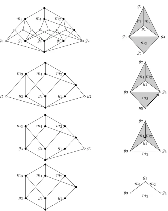
The idea of the proof is to perform the deformation through a number of intermediary easier reduction steps. To keep track of the changes performed in each step we will at the same time transform the lattice Γ(S_K) (belonging to S_K) into the lattice B_K (belonging to ∆(B_K)). Thus the deformation of the simplicial complex S_K into the simplicial complex ∆(B_K) will be performed simultaneously with a simplification of lattices to be defined in the sequel, starting with the lattice Γ(S_K) and ending in the lattice B_K. For a first glimpse of this process we refer to figure 2. The reduction relation on lattices (or rather bounded posets, since the intermediary objects do not need to be lattices) will have the following properties:

(i) We can reduce the lattice Γ(S_K) to the lattice B_K via a finite number of intermediary bounded posets.

(ii) If L reduces to L0 in one reduction step then the simplicial complex ∆(L0) is a strong deformation retract of the simplicial complex ∆(L).

By consecutively applying a finite number of strong deformation retractions one obtains again a strong deformation retraction. Thus from (i) and (ii) we get a strong deformation retraction from ∆(Γ(S_K)) to ∆(B_K). The desired theorem follows since we have ∆(Γ(S_K)) = S_K by proposition 4.4.

We start to elaborate the proof just sketched by defining the described reduction relation between posets. The term “reflexive and transitive closure” to be found in the definition means that we also allow multiple (including zero) reduction steps performed in a row.

Definition 6.1. Let L be a poset and K a subset of L. Define one-step reduction →K of L

with respect to K by the clause

L →K L\{x} if x is a maximal element of L\K.

Let →∗_K be the reflexive and transitive closure of →K. If L →∗K L0 holds we say that L0 is a

K-reduct of L.

To see an example consider the second lattice from the top in the left column of figure 2. For K take the set of black filled nodes. Then the atom labelled g5 is a maximal node which

is not in K, so removing this node is a one-step reduction of the lattice. The result of the reduction step is the lattice below, i.e. the third lattice from the top in the same figure. As for motivation, we will apply the definition always with a set K which is closed under meets. Then maximality of x implies that x can have at most one upper neighbour, which will turn out to be important in the proofs to come. Since we are only dealing with finite posets the following lemma is easy to show: As long as there is a node of the lattice which is not in K there is a maximal node with this property, so we can remove it until eventually all remaining nodes are in K.

Lemma 6.2. We have L →∗_K K for any poset L and any subset K of L.

Recall the function ζ : B_K → Γ(S_K) from the precedent section. The image ζ(B_K) of B_K under that function is a subset of the lattice Γ(S_K). If we take L = Γ(S_K) and K = ζ(B_K)

in the precedent lemma, then we obtain Γ(S_K) →∗_ζ(B

K) ζ(BK). Recall also that ζ is an order

embedding, thus an order isomorphism onto its image. This gives the following corollary that corresponds to point (i) above.

Corollary 6.3. The lattice B_K is a ζ(B_K)-reduct of Γ(S_K), up to the renaming of nodes. It remains to elaborate point (ii) above: We have to show that if L reduces to L0 in one reduction step then the simplicial complex ∆(L0) is a strong deformation retract of the simplicial complex ∆(L). Let us first look at an example: For L and L0 take the third and fourth lattice from the top in the left column of figure 2. The subset K ⊂ L consists of the nodes marked black. The reduction step from L to L0 consists in removing the atom g2,

which is a maximal node not in K. How does this reduction affect the simplicial complexes belonging to the two lattices (right column of the figure)? Removing the atom g2 from the

lattice L means removing the vertex g2 from the simplicial complex ∆(L). We have to show

that this results in a strong deformation retraction. Now the atom g2 has a special role in the

lattice L: There is a second atom, namely g1, which lies below any co-atom above g2 (these

co-atoms are m1 and m2). In terms of simplicial complexes this means that any maximal

simplex in ∆(L) which contains g2 does also contain g1, and thus contains the whole edge

between g2 and g1. Consequently removing g2 can be achieved by a projection parallel to

that edge, i.e. by collapsing the edge between g2 and g1 to the single point g1. The fact that

every maximal simplex containing g2 contains the whole edge means that in doing so we do

not “destroy” any holes of the simplicial complex. We now give the general proof.

Lemma 6.4. Let L be a bounded poset and K a subset of L that contains 0, 1 and all co-atoms. Suppose also that any two elements of K have a meet that is itself an element of K. Then L →K L0 implies that ∆(L0) is a strong deformation retract of ∆(L).

Proof. Let x be the maximal element of L\K such that we have L0 = L\{x}. Suppose first that x is not an atom of L. Then ∆(L0) is equal to ∆(L): Any set of atoms that is bounded in L by an element different from 1 is bounded by a co-atom, and since x cannot be a co-atom this bound is still present in L0. Now suppose that x is an atom. Then x has exactly one upper neighbour in L: For suppose that it has two. By maximality of x they would both have to be in K. Since K is closed under meets this implies that x is itself in K, contrary to what we have assumed. Write y for the only upper neighbour of x. If x is the only atom below y then y will replace x as an atom in L0 and ∆(L0) will be equal to ∆(L), modulo renaming the vertex x into y. Now consider the case where z is an atom below y that is different from x. Consider a geometric realization of ∆(L) in RN as described above: We choose z to be the origin, x the first unit vector and all other vertices points in the plane spanned by the remaining unit vectors. We will refer to the latter plane as the base plane. The passage from ∆(L) to ∆(L0) consists in deleting the vertex x and all simplices containing it. Thus in the geometric realization ∆(L0) is the part of ∆(L) which lies in the base plane.

Now x is not a co-atom and thus y is not equal to 1. Recall that y is the only upper neighbour of x and that z is below y. Thus any maximal simplex containing x must also contain z. Then the projection down to the base plane parallel to the first unit vector is a strong deformation retraction of ∆(L) onto ∆(L0).

Now to obtain the desired theorem it suffices to put the pieces together:

Theorem 6.5. Let K be a context, BK its concept lattice and SK its simplicial complex. Then

m3 m1 m2 g5 g3 g4 g1 g2 g2 g1 g3 g4 g5 m2 m1 m3 m3 m1 m2 g5 g3 g4 g1 g2 g2 g1 g3 g4 g5 m2 m1 m3 m3 m1 m2 g3 g4 g1 g2 g2 g1 g3 g4 m3 m2 m1 m3 m1 m2 g3 g4 g1 g1 g3 g4 m2 m1 m3

Figure 2: The proof of theorem 6.5 illustrated by the example from figure 1. Left from top to bottom: Reduction of the lattice Γ(S_K) to the concept lattice B_K. The latter lattice can be embedded into the first via the map ζ depicted in figure 1. The nodes in the image of this map are filled black. One passes from the uppermost to the lowermost lattice by removing maximal non-filled nodes, one at a time. — Thus in fact there should be seven steps between the first and the second lattice. Right: Each simplicial complex is the image of the lattice left to it under the map ∆. The labels serve to retrace this association: Atoms and co-atoms of the lattices become vertices and maximal simplices of the simplicial complexes respectively. The uppermost simplicial complex is (∆ ◦ Γ)(S_K) = S_K, and the lowermost is ∆(B_K). As proved in the text for the general case, each simplicial complex is a strong deformation retract of the simplicial complex above it. An arrow indicates a retraction that will occur in the next step. The retraction should be imagined as a projection parallel to the arrow.

Proof. First note the following: If K satisfies the conditions of the precedent lemma with respect to L and if we have L →K L0 then K satisfies the same conditions with respect to

L0. As a consequence the lemma holds with →∗_K as well as with →K. Proposition 5.2 tells us

that ζ(B_K) ⊂ Γ(S_K) satisfies the conditions of the precedent lemma. Together with corollary 6.3 this implies that ∆(B_K) is a strong deformation retract of ∆(Γ(S_K)). The theorem follows because ∆(Γ(S_K)) is equal to S_K by proposition 4.4.

That ∆(B_K) is a strong deformation retract of S_Kmeans in particular that the two simpli-cial complexes are homotopy equivalent, i.e. agree on many important topological properties. This gives a decidedly positive answer to the question posed in section 2: Is it possible to read off interesting information about the simplicial complex S_K from (the isomorphism class of) the concept lattice B_K alone? We can now say that yes, in a very precise sense this is the case: All homotopy invariant properties of S_K can be determined from B_K alone. To do so, simply compute the lattice complex ∆(B_K) and determine which properties this simplicial complex has. As we have just seen, the homotopy invariant properties for this simplicial complex are equal to those one would obtain from S_K itself. Thus for example the concept lattice includes enough information to determine whether the simplicial complex is connected and whether all loops can be retracted to a single point. It also allows to compute the homology groups and in particular the Betti numbers, which constitute a strong invariant of topological spaces and are algorithmically computable in the case of finite simplicial complexes.

7

Formal concept analysis and simplicial complexes in music

In this section and the next, we will give an application of theorem 6.5 in the context of mathematical music theory.

We look at sequences of pitches that have some internal symmetries, called Messiaen’s Modes of Limited Transpositions (MLT). Such sequences have been characterized using group-theoretic notions. The idea to analyze musical objects using the tools of group theory is now largely developed in mathematical music theory but some natural musical objects cannot be easily modeled in this way. This shortcoming leads to generalizations relying on alternative representations: topology and lattice related structures make possible the formalization of musical objects with less symmetries. In the following, we give a topological characterization of the maximal MLT. This topological characterization follows the work started in [Cat11, BGS11] and contributes to the task of “lifting” the results known in the group-theoretic setting to the more general topological framework. In establishing the characterization of maximal MLT, the theorem 6.5 is instrumental because it simplifies some computations.

The rest of this section introduces the context of mathematical music theory, the group theoretic approach and the emerging topological approach. Then, paragraph 7.2 presents the notion of MLT through some elementary examples. Section 8 is devoted to the study of the topological representation of MLT with simplicial complexes, and their topological characterization.

7.1 Mathematical music theory and the study of sequences of pitches

The relationships between mathematics and music are an age old story and go back at least to the Pythagoreans who have investigated the expression of musical scales in terms of numerical ratios. Current research in this field still focuses on the uses of mathematical structures to

analyze, characterize and reconstruct musical objects. Musical objects have often a highly combinatorial structure and their mathematical formalization allows for their enumeration and classification. In this context, the study of a sequence of pitches3 is of special interest because numerous musical objects lead naturally to a sequence of pitches: chord, scale, mode, melody, etc. In a first approach, two main paths have been followed for the classification of sequence of pitches, relying on group-theoretic or topological tools used in their modeling.

Inspired by the work of Hugo Riemann [Reh03], music theorists began in the 1980s to use techniques from group theory to analyze sequences of pitches. David Lewin [Lew87] introduced generalized interval systems to study the properties of a set of pitches under several musical transformations seen as (simply) transitive group actions. This idea abstracts many formalizations of musical objects and leads naturally to classifications relying on group equivalences and group classifications. And indeed, the problem of the enumeration and classification of chords having different kinds of inner symmetries and with respect to different group actions has been a major research area in mathematical music theory, from Halsey and Hewitt’s inaugural paper [HH78] until the more recent contributions by music theorists from the computational musicological community, such as Nick Collins [Col12]. Contributions in this area include David Reiner’s enumerations of set and row classes [Rei85] and Harald Fripertinger’s investigations of chords and motifs [FV92], mosaics [Fri99b] and canons [Fri99a]. Although algebraic in nature, the group structures underlying these approaches may re-ceive a geometric interpretation. More recently, Guerino Mazzola [MMH90, M+02], Dmitri Tymoczko [Tym06] and others have developed the geometric approach for itself and identified many geometric spaces that arise naturally in music and such that musical transformations between the relevant objects cannot be easily modeled by a group action. Providing a compre-hensive account of these developments is clearly out of the scope of this article. It is however interesting to briefly discuss some relevant sources on the application of formal concept anal-ysis and simplicial complexes in music theory.

One of the first uses of simplicial complexes in music theory was developed by G. Mazzola with the notion of “global compositions”. A global composition is a particular atlas of local charts, a chart referring to some relevant musical notions, which are glued together and to which one can associate a topological structure, the nerve, as a simplicial complex. One of the motivating examples is the M¨obius strip which is associated to the covering of the diatonic space by chords built on its seven degrees. In Mazzola’s original approach as introduced in [Maz85] and later developed in [MMH90], the charts of a given atlas are represented as 0-simplices and the n-dimensional 0-simplices correspond to non-empty n-fold intersections of the elementary charts. There are alternative ways of associating simplicial complexes to music, by taking the notes as 0-simplices and chords with n notes as n-simplices, as suggested by Louis Bigo et. al [BGS11, BAG+13] as well as Michael Catanzaro [Cat11]. The result presented here takes place in this framework.

These approaches are rooted in algebraic topology and emphasize the use of combinatorial notions. Metric properties can be included, e.g. to take into account timing information. This path has been proposed by Andreas Nestke [Nes04] to study the space of musical melodies taking into account the onset of each note. Melodies are studied as finite ordered sets of rational points in the affine plane, each point describing the pitch but also the duration of

3

It is customary to consider equivalent pitches that are a whole number of octaves apart. Such equivalence classes are also called chromas or pitch classes. Considering 12 notes in an octave, pitch classes are typically represented as numbers in Z12, but for the formalization we consider Znfor any n.

each note. The author proposes then to make use of homology as a general tool to classify the simplicial complex. This is in contrast with the characterization of MLT we develop in the next section, where the classification is based on homotopy.

Considering the recurrent quest of classification tools in mathematical music theory, it is surprising that FCA is not more significant in the field. However, the two domains have a long shared history. Although there is no mention of music in Wille’s inaugural article on the reconstruction of lattice theory [Wil82], one may reasonably argue that music was a major inspirational field for applying formal concept analysis to concrete situations. In fact, the first tables of musical objects and attributes appeared just few years after this article and they are accompanied by their concept lattice representations which show the way in which harmonies are organized within the traditional diatonic system corresponding to the white-keys of the piano keyboard [Wil85]. This modeling is clearly providing the major theoretical framework for the successive attempt at establishing a functorial morphology of musical chords by the members of the Research Group KIT-MaMuTh in Berlin. Actually, the notion of morphology of musical chords, as introduced in [NB04], is based on the notion of Harmonic Morphemes which are conceived as formal concepts consisting of a collection of affine transformations (also called the tone perspectives) and a set of chords. The set of tonal perspectives and chords play respectively the role of intension and extension of harmonic morphemes whose harmonic (intension and extension) topology is a special case, as the authors point out, of the much more general situation of functorial local compositions and their endomorphisms, as introduced by Guerino Mazzola in his topos-theoretical approach [M+02, chap. 24].

The issue of associating concept lattices with paradigmatic approaches in the classification of musical structures has been recently addressed by [SA13]. In this article FCA is applied to the algebraic enumeration, classification and representation of subsets of the Tone System according to an equivalence relation obtained either via an action of a given finite group on the collection of subsets of it or via an identification of their intervallic content (such as Allen Forte’s interval vector [For73] or David Lewin’s interval function [Lew77]).

7.2 Messiaen’s modes of limited transpositions

In this paragraph we present Olivier Messiaen’s modes of limited transpositions (MLT). The topological classification of MLT, which offers a nice example of interplay between concept lattices and associated simplicial complex representations, is addressed in the next section.

Studied by the French composer Olivier Messiaen and published in his book La technique de mon langage musical, an MLT is a subset of the 12 notes that has strictly less than 12 different transpositions. In other words, an MLT is a subset of notes such that there exists a non trivial transposition that leaves the subset invariant.

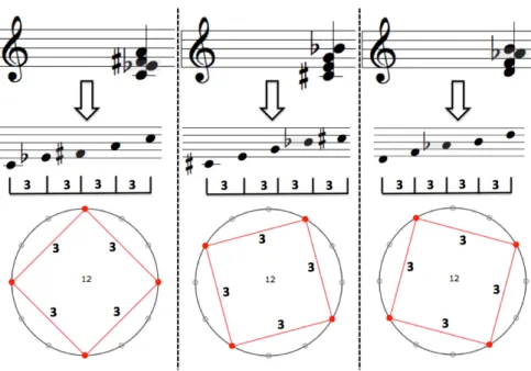
MLT are a well-known historical example of musical structures whose underlying trans-positional symmetry property can be easily described in terms of group actions and algebraic combinatorics [Rea97, Bro01]. Musically speaking, MLT are equivalent to chords whose in-tervallic structure, i.e. whose sequence of intervals between two successive elements of the chord, is redundant. This means that the intervallic structure has an inner periodicity which explains the fact that they can musically be transposed only a limited number of times. The most elementary example of MLT is provided by chords or musical scales corresponding to regular polygons inscribed in a circle, such as the diminished tetrachord represented in Fig. 3. In this case, the intervallic structure only contains one interval, which is repeated a number

Figure 3: An example of MLT corresponding to a regular polygon inscribed in a circle. The associated musical object has an intervallic structure which is just the repetition of a given interval a number of times equal to the number of notes, i.e. (3 3 3 3). Note that this MLT admits three possible transpositions, meaning that the associated polygon can only be rotated three times (including the identity transformation) before superposing to itself. (Diagrams in Fig. 3, 4 and 5 are generated using the generalized interval toolbox available in OpenMusic [BAA11].)

of times equal to the number of notes. From a mathematical point of view, this first case cor-responds to the subgroups of Z12. In the more general case, MLT can be described as subsets

of the cyclic group of order n which are not necessarily subgroups but are invariant up to an element of this group which is different from the identity. This second case is represented in Fig. 4 and corresponds to the so-called octatonic mode alternating semi-tones and whole-tone steps.

We call a harmonic form a maximal MLT with m transpositions if none of the harmonies representing it is strictly contained in another mode with m transpositions. The diminished tetrachord in Fig. 3 is not maximal since one of its three harmonies is strictly contained in the octotonic mode. On the contrary, this latter is a maximal MLT, since there is no MLT with three transpositions which strictly includes the octotonic mode. The interested reader can easily check that among the MLT which are associated to subgroups of Z12, the only one

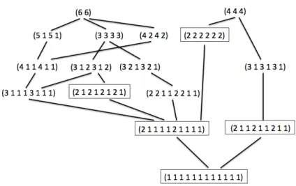
which is maximal is the whole-tone scale with intervallic structure equal to (2 2 2 2 2 2 2 2). The inclusion lattice of the family of 16 MLT (including the whole space Z12) is shown in

Fig. 5.

8

Simplicial complexes of modes of limited transposition

In order to understand this group-theoretical property, let us introduce a small amount of musical terminology we take from [SS10]. The basic entity we are working with is the group Zn, which we call the n-tone equal tempered chroma system, or chroma system for short, in

this context. The most important example in music theory is n = 12, corresponding to the twelve semi-tones of the chromatic scale. Elements of Zn are called chromas and subsets of

Zn are called harmonies. Now the group Zn appears in a second role, namely as acting on

the set P(Zn) of harmonies by element-wise addition modulo n, that is by the rule

(k, H) 7→ H + k = {m + k mod n | m ∈ H}

for H ∈ P(Zn) and k ∈ Zn. The element k ∈ Zn is called an interval when it appears in

this role. For fixed k the mapping H 7→ H + k is called a transposition by k. The orbit of a harmony under this group action is called a harmonic form. A harmony which is an element of a harmonic form is said to represent the latter. Using this terminology it is easy to define modes of limited transposition.

Definition 8.1. A harmonic form is said to have m transpositions if there are exactly m different harmonies that represent it. A mode of limited transposition in Zn, or mode for

short, is a harmonic form that has more than one but less than n transpositions.

One can easily establish a correspondence between modes with m transpositions and harmonic forms in Zm: If Zn allows for a mode with m transpositions then, by the orbit–

stabilizer theorem, m devides n. In this case the natural projection π : Z → Zm descends

to a group homomorphism π : Zn → Zm. Then π−1 : P(Zm) → P(Zn) is a mapping from

harmonies in Zm to harmonies in Zn. One can view π−1 as acting on harmonic forms by

element-wise application

H 7→ {π−1(H) | H ∈ H}.

The following lemma shows how this application connects modes of limited transposition with m transpositions and harmonies in Zm.

Figure 4: A MLT whose intervallic structure is equal to (1 2 1 2 1 2 1 2), i.e. it is four times the repetition of the sub-pattern (1 2). Note that the sum of the elements of the sub-pattern is equal to 3, meaning that the associated musical object has three possible transpositions, as in the case of Fig. 3

Figure 5: There are 16 MLT in Z12, including the chromatic scale which corresponds to the

entire support space Z12. This inclusion lattice shows the five maximal MLT, each mode

Lemma 8.2. If H is a harmonic form in Zm then π−1(H) is a harmonic form with |H|

transpositions in Zn. Any harmonic form in Znsuch that its number of transpositions divides

m arises in this way.

Proof. For h ∈ Zn we have the equivalence π(h) ∈ H + π(k) ⇔ π(h − k) ∈ H, which gives

the equality

π−1(H + π(k)) = π−1(H) + k

for any harmony H in Zm and any k ∈ Zn. The elements of the harmonic form H are of the

form H + k for some common harmony H representing H and for k = 0, . . . , m − 1. Then the elements of π−1(H) are precisely the harmonies π−1(H) + k for k = 0, . . . , n − 1, which shows that π−1(H) is a harmonic form. Since π : Zn→ Zm is surjective, the mapping π−1 between

harmonies is injective, that is we have |π−1(H)| = |H|. Suppose on the other hand that H is a harmonic form in Zn such that its number of transpositions divides m. Then H + m = H

holds for any harmony representing it. One easily deduces H = π−1(π(H)), where π(H) is to be understood as element-wise application. This gives H = π−1(π(H)). Finally π(H) is a harmonic form in Zm since we have π(H + k) = π(H) + π(k) for any harmony H in Zn and

any k ∈ Zn.

In particular π−1(H) is a mode of limited transposition if and only if |H| is bigger than 1 and smaller than n. If we have m < n then this is true if H is neither {∅} nor {Zm}.

We use the theoretic results obtained so far to investigate simplicial complexes that are associated to modes of limited transposition in a similar way. But first of all let’s see how to associate a concept lattice to the family of Messiaen’s limited transposition modes.

A harmonic form can be represented by a formal context in the following way.

Definition 8.3. Let H be a harmonic form in Zn. The associated formal context is given by

KH= (Zn, H, I), where (h, H) ∈ I is by definition equivalent to h ∈ H.

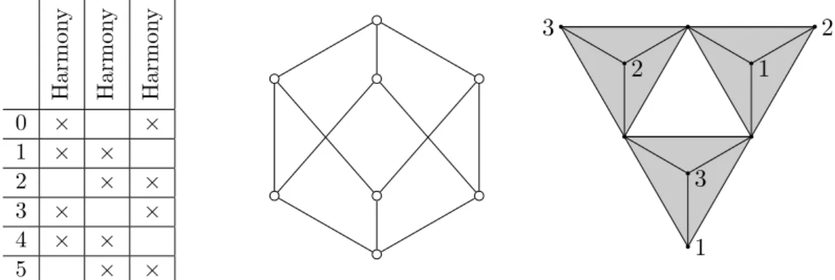
To such a context we can associate a concept lattice and a simplicial complex, as is done in figure 6 for the case of a mode with three transpositions in the chroma system Z6. We want

to investigate these objects for harmonic forms that are modes of limited transposition. It turns out that the concept lattice has a rather simple structure while the simplicial complex is hard to visualise already in our small example. We can however determine its homotopy type using the theoretic results of the previous sections.

To make this precise reconsider our above discussion of the projection π : Zn→ Zm. The

following proposition expresses the fact that this mapping preserves the concept lattice, as well as most topological properties of the simplicial complex associated to a harmonic form.

Proposition 8.4. Let H be a harmonic form in Zm. The concept lattices BKH and BKπ−1(H)

are equal. The simplicial complexes S_KH and SKπ−1(H) are homotopy equivalent.

Proof. Passing from Kπ−1_(H) to K_H consists in deleting all but the first m objects of the

context. Since H + m = H holds for any harmony H representing π−1(H) we only delete objects that have a “double” which has the same attributes. In the language of formal concept analysis this is a special case of deleting a reducible object (see [GW99]). Considering concepts this object is accordingly deleted from all extents. However, as the double is still present, the intents of the concepts do not change. Thus the structure of the concept lattice is preserved,

Harmon y 1 Harmon y 2 Harmon y 3 0 × × 1 × × 2 × × 3 × × 4 × × 5 × × 1 3 2 3 2 1

Figure 6: The context associated to a mode with three transpositions in the chroma system Z6,

its concept lattice and its simplicial complex. The latter consists of three tetrahedra, which should be embedded into some RN such that vertices with the same label are identified. If we consider the first three lines of the context only, then the concept lattice stays the same. As simplicial complex we get the boundary of a triangle, thus a space isomorphic to the circle S1. As shown in the text the latter is homotopy equivalent to the full simplicial complex depicted in the figure.

i.e. we have B_KH = BKπ−1(H). The statement concerning the simplicial complexes follows by

applying theorem 6.5: S_KH is homotopy equivalent to ∆(BKH). This is equal to ∆(Bπ−1(H))

which in turn is homotopy equivalent to S_π−1_(H).

Note that we could have shown a slightly stronger result by directly applying the methods used in the proof of lemma 6.4: Omitting objects that have a double amounts to performing a strong deformation retraction in the corresponding simplicial complexes. Thus in fact S_K

π−1(H) is even a strong deformation retract of SKH.

With this result at hand it is particularly easy to compute the homotopy type of the simplicial complex associated to a maximal mode of limited transposition. We call a harmonic form a maximal mode with m transpositions if none of the harmonies representing it is strictly contained in another mode with m transpositions.

Corollary 8.5. Let H be a maximal mode with m transpositions. Then its associated sim-plicial complex S_KH is homotopy equivalent to the sphere S

m−2_.

Proof. By lemma 8.2 there is a harmonic form H0 in Zm which satisfies H = π−1(H0). Since

H is a maximal mode with m transpositions the harmonic form H0 is represented by maximal non-trivial harmonies in Zm. In other words the harmonies representing it are precisely the

harmonies which contain all but one chroma. Thus the simplicial complex associated to the context KH0 is the boundary of a (m − 1)–simplex, which is homeomorphic to the sphere

Sm−2. The result follows by the precedent proposition.

9

Conclusions and further work

On the theoretic side we wanted to establish a connection between two approaches to the analysis of a binary relation: by formal concept analysis and via simplicial complexes. As a foundation for such a comparison we have defined an association between lattices and

simplicial complexes. On this basis we have shown that the concept lattice arising from formal concept analysis contains enough information to reconstruct any homotopy invariant property of the simplicial complex corresponding to the same context. Examples for such properties are connectedness, homotopy groups, homology groups and Betti numbers. While the concept lattice contains information about all these topological properties, they may not be easy to perceive when looking at the lattice alone. The use of simplicial complexes can thus be seen as a factual extension of the methods of formal concept analysis, without that it would transcend them in principle. Some properties of the simplicial complex, such as dimension, cannot be reconstructed from the form of the concept lattice. Depending on the application in question they may constitute a relevant additional point of information.

The theoretic result can be used in a number of different ways, ranging from general proofs to concrete applications: In the proof of proposition 8.4 we have used the fact that certain modifications of a context leave the concept lattice unchanged to show that they do not change the homotopy type of the simplicial complex either. In a concrete application topological properties of the simplicial complex, such as the presence of several connected components, may suggest to split the data in a certain way. The concept lattices associated to the different components may well be more intelligible than the lattice built from the whole context.

There is much work to be done on the theoretic side: Firstly one might want to explore in more detail which properties of the concept lattice can be recovered from the simplicial complex. In addition, alternative representations can be built by duality (e.g. by exchanging the role of objects and attributes). The systematic study of the relationships between these representations remains to be done. Secondly it will be important to see how decomposition methods of the concept lattice on the one and of simplicial complexes on the other hand behave with respect to our comparison. Decomposition methods are an important tool in formal concept analysis to produce concept lattices that are small enough to be instructive. In some applications concept lattices are very suitable to represent the global structure of the data while local symmetries are well captured by simplicial complexes. In order to develop decomposition techniques, which provide a link between the local and the global, it thus seems promising to take both viewpoints into account. As a concrete starting point we would like to study the connection between simplicial complexes and concept lattice orbifolds, a technique to “fold” concept lattices using symmetries of the context, which has been introduced by Daniel Borchmann and Bernhard Ganter [BG09].

As for applications to music theory we have seen how the combination of formal concept analysis and simplicial complexes can be used for a topological investigation of some highly symmetrical musical structures, such as Messiaen’s modes of limited transposition. In the long term it remains to inquire on the demand and feasibility of a comprehensive indexing of harmonies based on formal concept analysis and simplicial complexes.

Acknowledgements. The first author research work was developed while he was student at Ludwig–Maximilians–Universit¨at, (Munich), during an internship at IRCAM.

Anton Freund wants to thank the Institut de Recherche et Coordination Acoustique / Musique (IRCAM) for welcoming him as a guest researcher and thus making the joint research pre-sented in this paper possible. He also wants to thank the foundation Stiftung Maximilianeum and the German National Merit Foundation (Studienstiftung des deutschen Volkes) for sup-porting this research stay in Paris.

The authors are also grateful to the anonymous reviewers for their valuable comments and suggestions to improve the quality of a first version of this paper.

References

[Atk72] Ronald H. Atkin. From cohomology in physics to q–connectivity in social science. Int. J. Man Mach. Stud., 4(2):139–167, 1972.

[Atk78] Ronald H. Atkin. Q-analysis. A hard language for the soft sciences. Futures, pages 492–499, 1978.

[BAA11] Jean Bresson, Carlos Agon, and G´erard Assayag. Openmusic: visual programming environment for music composition, analysis and research. In Proceedings of the 19th ACM international conference on Multimedia, pages 743–746. ACM, 2011.

[BAG+_{13] Louis Bigo, Moreno Andreatta, Jean-Louis Giavitto, Olivier Michel, and Antoine}

Spicher. Computation and visualization of musical structures in chord-based sim-plicial complexes. In Jason Yust, Jonathan Wild, and John Ashley Burgoyne, editors, Mathematics and Computation in Music, volume 7937 of Lecture Notes in Computer Science, pages 38–51. Springer Berlin Heidelberg, 2013.

[BG09] Daniel Borchmann and Bernhard Ganter. Concept lattice orbifolds — first steps. In S. Ferr´e and S. Rudolph, editors, Formal Concept Analysis: 7th International Conference, ICFCA 2009 Darmstadt, Germany, May 21–24, 2009 Proceedings. Springer Verlag, Berlin and Heidelberg, 2009.

[BGS11] Louis Bigo, Jean-Louis Giavitto, and Antoine Spicher. Building topological spaces for musical objects. In Mathematics and Computation in Music, volume 6726 of LNCS, Paris, France, Juin 2011. Springer.

[BKLW01] H´elene Barcelo, Xenia Kramer, Reinhard Laubenbacher, and Christopher Weaver. Foundations of a connectivity theory for simplicial complexes. Advances in Applied Mathematics, 26(2):97–128, 2001.

[BM70] Marc Barbut and Bernard Monjardet. Ordre et classification : alg`ebre et combi-natoire. Hachette, 1970.

[Bro01] Michel Brou´e. Les tonalit´es musicales vues par un math´ematicien. Le temps des savoirs (Revue de l’Institut Universitaire de France), pages 37–78, 2001. Odile Jacob.

[Cas79] John L Casti. Connectivity, complexity, and catastrophe in large-scale systems. J. Wiley New York, 1979.

[Cat11] Michael J Catanzaro. Generalized Tonnetze. Journal of Mathematics and Music, 5(2):117–139, 2011.

[Col12] Nick Collins. Enumeration of chord sequences. In Sound and Music Computing, Aalborg University Copenhangen, Denmark, 2012. SMC.