HAL Id: hal-01446792
https://hal.archives-ouvertes.fr/hal-01446792
Submitted on 20 Dec 2017
HAL is a multi-disciplinary open access
archive for the deposit and dissemination of
sci-entific research documents, whether they are
pub-lished or not. The documents may come from
teaching and research institutions in France or
abroad, or from public or private research centers.
L’archive ouverte pluridisciplinaire HAL, est
destinée au dépôt et à la diffusion de documents
scientifiques de niveau recherche, publiés ou non,
émanant des établissements d’enseignement et de
recherche français ou étrangers, des laboratoires
publics ou privés.
Distributed under a Creative Commons Attribution| 4.0 International License
A small-scale hyperacute compound eye featuring active
eye tremor: application to visual stabilization, target
tracking, and short-range odometry
Fabien Colonnier, Augustin Manecy, Raphaël Juston, Hanspeter Mallot,
Robert Leitel, Dario Floreano, Stéphane Viollet
To cite this version:
Fabien Colonnier, Augustin Manecy, Raphaël Juston, Hanspeter Mallot, Robert Leitel, et al.. A
small-scale hyperacute compound eye featuring active eye tremor: application to visual stabilization,
target tracking, and short-range odometry. Bioinspiration and Biomimetics, IOP Publishing, 2015, 10
(2), pp.26002. �10.1088/1748-3190/10/2/026002�. �hal-01446792�
Fabien Colonnier1, Augustin Manecy1,2, Raphaël Juston1, Hanspeter Mallot3, Robert Leitel4,
Dario Floreano5and Stéphane Viollet1,6
1 Aix-Marseille Université, CNRS, ISM UMR 7287, 13288, Marseille cedex 09, France
2 GIPSA-lab laboratory, Control Systems Dept., SySCo team, CNRS-Univ. of Grenoble, ENSE3 BP 46, 38402 St Martin d’Hères Cedex,
France
3 Laboratory of Cognitive Neuroscience, Department of Biology, University of Tübingen, 72076 Tubingen, Germany 4 Fraunhofer Institute for Applied Optics and Precision Engineering, 07745 Jena, Germany
5 Laboratory of Intelligent Systems, École Polytechnique Fédérale de Lausanne, CH-1015 Lausanne, Switzerland 6 Author to whom any correspondence should be addressed.
E-mail:fabien.colonnier@univ-amu.fr,augustin.manecy@univ-amu.fr,rjuston@avenisense.com,hanspeter.mallot@uni-tuebingen. de,robert.leitel@iof.fraunhofer.de,dario.floreano@epfl.chandstephane.viollet@univ-amu.fr
Supplementary material for this article is availableonline
Abstract
In this study, a miniature artificial compound eye (15 mm in diameter) called the curved artificial
compound eye (CurvACE) was endowed for the first time with hyperacuity, using similar
micro-movements to those occurring in the fly’s compound eye. A periodic micro-scanning movement of
only a few degrees enables the vibrating compound eye to locate contrasting objects with a 40-fold
greater resolution than that imposed by the interommatidial angle. In this study, we developed a new
algorithm merging the output of 35 local processing units consisting of adjacent pairs of artificial
ommatidia. The local measurements performed by each pair are processed in parallel with very few
computational resources, which makes it possible to reach a high refresh rate of 500 Hz. An aerial
robotic platform with two degrees of freedom equipped with the active CurvACE placed over
natu-rally textured panels was able to assess its linear position accurately with respect to the environment
thanks to its efficient gaze stabilization system. The algorithm was found to perform robustly at
differ-ent light conditions as well as distance variations relative to the ground and featured small closed-loop
positioning errors of the robot in the range of 45 mm. In addition, three tasks of interest were
per-formed without having to change the algorithm: short-range odometry, visual stabilization, and
track-ing contrasttrack-ing objects (hands) movtrack-ing over a textured background.
1. Introduction
According to the definition originally proposed by Westheimer in 1975 [1] and recently reformulated in 2009 [2]: ‘Hyperacuity refers to sensory capabilities in which the visual sensor transcends the grain imposed by its anatomical structure’. In the case of vision, this means that an eye is able to locate visual objects with greater accuracy than the angular difference between two neighboring photoreceptorsΔφ. This study pre-sents the first example of an artificial compound eye that is able to locate the features encountered with much greater accuracy than that imposed by its optics
(i.e.,Δφ). Based on findings originally observed in fly vision, we designed and constructed an active version of the previously described artificial compound eye CurvACE [3,4]. Active CurvACE features two proper-ties usually banned by optic sensor designers because they impair the sharpness of the resulting images: optical blurring and vibration. The active visual principle applied here is based on a graded periodic back-and-forth eye rotation of a few degrees scanning the visual environment. Scanning micro-movements of this kind have been observed in humans [5] and several invertebrates such as crabs [6], molluscs [7], and arachnids [8,9].
19 December 2014
ACCEPTED FOR PUBLICATION
9 January 2015
PUBLISHED
25 February 2015 Content from this work may be used under the terms of theCreative Commons Attribution 3.0 licence.
Any further distribution of this work must maintain attribution to the author (s) and the title of the work, journal citation and DOI.
The first micro-scanning sensor based on the peri-odic retinal micro-movements observed in the fly (for a review, see [10]) was presented in [11], whereas recent developments [12–14] have led to the imple-mentation of bio-inspired vibrating sensors endowed with hyperacuity. However, hyperacuity has also been obtained in artificial retinas without using any retinal micro-scanning processes, based on the overlapping Gaussian fields of view of neighboring photosensors (for a review, see [15]). The authors of several studies have assessed the hyperacuity of an artificial com-pound eye in terms of its ability to locate a point source [16], a bar [17], a single line [18] (the bar and the line both take the form of a stripe in the field of view (FOV)), an edge [19], and to sense the edge’s orienta-tion [20]. The robustness of these visual sensors’ per-formances with respect to the contrast, lighting conditions, and distance from the object targeted (contrasting edges or bars) has never been assessed prior to the present study involving the use of a retinal micro-scanning approach. However, assuming that a priori knowledge is available about the targets and obstacles’ contrast, Davis et al [21] implemented effi-cient target tracking and obstacle avoidance behaviour onboard a ground-based vehicle equipped with a bulky apposition eye consisting of an array of 7 ommatidia.
As Floreano et al [3] have shown, an artificial curved compound eye can provide useful optic flow (OF) measurements. In addition, we established here that an artificial compound eye performing active per-iodic micro-scanning movements combined with appropriate visual processing algorithms can also be endowed with angular position sensing capabilities. With this visual sensing method, an aerial robot equipped with active CurvACE was able to perform short-range visual odometry and track a target moving over textured ground. The bio-inspired approach used here to obtain hovering behaviour differs completely from those used in studies involving the use of compu-ter vision or OF flow.
In this context, it is worth quoting, for example, two recent studies using binocular vision [22] and monocular vision [23] to perform hovering without any drift and visual odometry, respectively. However, the latency (about 18 ms) of the embedded visual pro-cessing algorithms used by the latter authors still limits the reactivity of the supporting aerial robotic platform. Other strategies combined visual cues with barometric data to obtain a visual odometer [24] or with an ultra-sonic range finder to implement a hovering autopilot [25]. In the case of hovering behaviour, many studies have been based on the assumption that the robots in question have previous knowledge of particular fea-tures present in the environment. Mkrtchyan et al [26] enabled a robot to hover using only visual cues by fix-ating three black rectangles, but its altitude was con-trolled by an operator. Likewise, landing procedures have been devised, which enabled robots equipped
with initial measurement unit (IMU)s and visual sen-sors to detect specific geometrical patterns on the ground [27] and [28]. Bosnak et al [29] implemented an automatic method of hovering stabilization in a quadrotor equipped with a camera looking downward at a specific pattern. Gomez-Balderas et al [30] stabi-lized a quadrotor by means of an IMU and two cam-eras, one looking downward and the other one looking forward. In the latter study, the OF was computed on the basis of the images perceived when looking down-ward and the robot’s position was determined by using a known rectangular figure placed on a wall, which was detected by the forward-facing camera.
OF has also been used along with IMU measure-ments to perform particular flight maneuvers such as hovering [31] and landing [32,33]. The robot devel-oped by Carrillo et al [34] rejected perturbations by integrating the OF with information about the height obtained via an ultrasonic range finder. In their experiments, the goal was to follow a path defined by a contrasting line.
Honegger et al [35] also developed an optical flow sensor for stabilizing a robotic platform hovering over a flat terrain, but the performances of this sensor over a rugged terrain or a slope were not documented. Along similar lines, Bristeau et al [36] developed a means to estimate the speed of a quadrotor by com-bining the speed given by an OF algorithm with that provided by an accelerometer.
The visual processing algorithm presented here estimates displacement by measuring the angular posi-tion of several contrasting features detected by active CurvACE. In this respect, this method differs com-pletely from those used in previous studies based on the use of the OF, which are similar to speed estimation methods.
The active version of the CurvACE sensor and the fly’s retinal micro-movements are described in section2.1, and a model for the vibrating eye, includ-ing its special optics, is presented in section2.2. The visual processing algorithms resulting in hyperacuity are described in section3. A complete description of the implementation of this sensor on a tethered robot named HyperRob is given in section4, and the robotʼs capability to assess its own linear position relative to the environment and track a target thanks to the active CurvACE, based on the novel sensory fusion algo-rithm developed here, is established in section5(see also section3.3).
2. Description of the visual sensor: active
CurvACE
2.1. Inspiration from the fly’s visual micro-scanning movements
In this study, visual hyperacuity results from an active process whereby periodic micro-movements are con-tinuously applied to an artificial compound eye. This
approach was inspired by the retinal micro-move-ments observed in the eye of the blowfly Calliphora (see figure 1(a)). Unlike the fly’s retinal scanning movements, which result from the translation of the photoreceptors (see figure1(b)) in the focal plane of each individual facet lens (for a review on the fly’s retinal micro-movements see [10]), the eye tremor applied here to the active CurvACE by means of a micro-stepper motor (figure 1(c)) results from a periodic rotation of the whole artificial compound eye. Section 2.3 shows in detail that both scanning processes lead to a rotation of the visual axis.
Here we describe in detail the active version of the CurvACE sensor and establish that this artificial com-pound eye is endowed with hyperacuity, thanks to the active periodic micro-scanning movements applied to the whole eye.
2.2. Modelling the optics
As described in [3], the CurvACE photosensors array has similar characteristics to the fruitfly eye in terms of the number of ommatidia (630), light adaptation, the interommatidial angle (Δφ = 4.2° on average), and a similar, Gaussian–shaped angular sensitivity function
Figure 1. (a) Head of a Calliphora vomitaria (Picture : J.J. Harrison, Wikimedia commons). (b) Top view of a fly’s head showing the orbito-tentorialis muscle (MOT, in red) attached to the back of the head (the fixed part : TT) and the base of the retina (the moving part : RET). The MOT is one of the two muscles responsible for the periodic retinal translation (for a review on the fly’s retinal micro-movements see [10]). Modified with permission from [37], copyright 1972 Springer. (c) The active CurvACE with its vibrating mechanism based on the use of a small stepper motor.
Figure 2. (a) Schematic view of a compound eye, showing the two main optical parameters of interest: the interommatidial angleΔφ, defined as the angle between optical axes of two adjacent ommatidia, and the acceptance angleΔρ, defined as the angle at half width of the Gaussian-shaped ASF. This particular shape of ASF results from the combination of the airy diffraction pattern and the geometrical angular width of the rhabdom at the nodal point of the lens [38]. The diameter of the facet lenses in the male blowfly Calliphora ranges from 20–40 μm, whereas that of the peripheral rhabdomeres is 1.5–2 μm (see [39] for review). Adapted with permission from [40], copyright 1977 Scientific American Inc. (b) CurvACE sensor and (c) the horizontal ASFs measured for each artificial ommatidium along the equatorial row (red line) (see [3] for further details). The mean value of the interommatidial angleΔφ
(ASF). This specific ASF removes ‘insignificant’ con-trasts at high spatial frequencies.
To replicate the characteristics of its natural coun-terpart (see figure2(a)), CurvACE was designed with a specific optical layer based on the assembly consisting of a chirped microlens array (lenslet diameter: 172 μm) and two chirped aperture arrays. In the case of active CurvACE, the optical characteristics remain constant during the scanning process.
Each ASF of active CurvACE (figures2(b) and (c)) can be characterized by the acceptance angle Δρ, which is defined as the angular width at half of the maximum ASF. The ASF along 1Ds ( ) of one Cur-ψ vACE ommatidium can therefore be written as fol-lows: ψ π πΔρ = − ψ Δρ s( ) 2 ln (2) e 4 ln(2) (1) 2 2
where ψ is the angle between the pixel’s optical axis and the angular position of a point light source. 2.3. Mathematical description of signals generated by vibrating ommatidia
Figures3(a) and (b) compare the rotation of the visual axes resulting from the translation of the retina behind a fixed lens (e.g., in the case of the fly’s compound eye) with the rotation of the visual axes resulting from the rotation of the whole eye (e.g., like the mechanism underlying the micro-saccades in the human’s camer-ular eye [41]), respectively. In the active CurvACE, we adopted the second strategy by subjecting the whole
eye to an active micro-scanning movement that makes the eye rotate back and forth.
As shown in figure3, the retinal micro-scanning movements are performed by a miniature eccentric mechanism based on a small stepper motor (Faulha-ber ADM 0620-2R-V6-01, 1.7 grams in weight, 6 mm in diameter) connected to an off-centered shaft [42]. This vibrating mechanism makes it possible to control the scanning frequency by just setting a suitable motor speed.
A general expression for the pixel’s output signal is given by the convolution of the ASFs ( ) with the lightψ intensity I of the 1D scene as follows:
∫
ψ = ψ ψ ψ ψ−
−∞ +∞
Ph( )c s( ) · (I c)d (2) whereψcis the angular position of a contrasting feature (edge or bar) placed in the sensor’s visual field. For example,I ( )ψ can be expressed for an edge as follows:
ψ = ψψ<⩾ I I I ( ) for 0 for 0 (3) 1 2 ⎧ ⎨ ⎩ and for a bar:
ψ = ψψ <⩾ I I L I L ( ) for 2 for 2 (4) 1 2 ⎧ ⎨ ⎩
with L the width of the bar (expressed in rad).
The micro-scanning movements of the pixels can be modelled in the form of an angular vibrationψmod of the optical axes added to the static angular position
ψc of the contrast object (an edge or a bar). The
equations for the two pixels (Ph1 and Ph2) are
Figure 3. Optical axis rotation resulting from (a) a micro-displacement ε of the pixels placed behind a fixed lens (e.g., in the case of a compound eye of the fly) or (b) a rotation of the whole sensor (e.g., in the case of the active CurvACE sensor). The micro-scanning of active CurvACE is subjected to active periodic rotational movements generated by a miniature eccentric mechanism. The angular vibrationψmodis generated by a miniature stepper motor represented here by an orange shaft and a purple off-centered shaft, which
translates along an elongated hole. The scanning frequency can be easily adjusted by changing the rotational speed of the motor. The scanning amplitude depends on the diameter of the off-centered shaft.
therefore: ψ = ψ +ψ − Δφ Ph( ( ))t Ph ( )t ( )t 2 (5) c mod 1 ⎜⎛⎝ ⎟⎞⎠ ψ = ψ +ψ + Δφ Ph ( ( ))t Ph ( )t ( )t 2 (6) c mod 2 ⎜⎛⎝ ⎟⎞⎠
withψmod obeying the following sinusoidal scanning
law:
ψmod( )t =A· sin 2
(
πfmod ·t)
(7) With A and fmoddescribing the amplitude and thefrequency of the vibration, respectively. In the case of a whole rotation of the eye, this scanning law is easily achievable by a continuous rotation of the motor with an off-centered shaft. In the case of a translation of the pixels behind a lens, the law should be weighted with the tangent of the ratio between the retinal displace-ment ε and the focal length f of the lens.
At the end, the photosensor response is a modu-lated convolution of the light intensity with the Gaus-sian sensitivity function.
3. Insights into the visual processing
algorithms
In this paper, we reuse the local processing unit (LPU) presented in [14] and apply the principle to active CurvACE. An LPU is an elementary pair of photo-sensors endowed with hyperacuity by means of a periodic vibration. The LPU is able to locate very accurately an edge or a bar placed in its small FOV. An artificial compound eye like CurvACE can provide several LPU outputs, which can be merged to obtain a bigger FOV and used as a basis for a higher level visual processing algorithm. In the following sections, we describe the different steps of the visual algorithm,
from the pixel processing to the novel fusion of the LPU’s output signals.
3.1. LPU: from photosensors to an accurate edge and bar location
The LPU defined in figure 4 is the application of algorithms presented in [13] and [14]. The first paper ([13]) leads to the signal OutputPosresulting from the
difference-to-sum ratio of the demodulated pixel output signals described by equation (8). The demo-dulation is realized by means of a peak filter that acts as both a differentiator and a selective filter centered at the scanning frequency (fp = fmod). Then, an absolute value function cascaded with a low-pass filter smooths out the pixel’s output signals. The second paper ([14]) explains in detail the edge/bar detection based on the observed phenomena that the two pixels’ output signals are in phase in the presence of an edge and in opposite phase in the presence of a bar. At the output of the LPU, the signalθirepresents the position of the contrasting feature in the FOV (see equation (9)).
= − + Output Ph Ph Ph Ph (8) Pos 1 2 1 2 demod demod demod demod
θ ψ = Outputi( )c Detector.OutputPos (9) With OutputDetectorequal to (−1) or (1) andθithe
output signal of an LPU (see figure4).
3.2. Hyperacute localization of contrasting bars and edges
The characteristic static curves of the active CurvACE obtained with a contrasting edge and a black bar 2.5 cm in width subtending an angle of 2.86° are presented in figure5.
The curve in figure5(a) has a tangent hyperbolic profile with respect to the angular position of the edge. It can be clearly seen by comparing the two curves
Figure 4. Block diagram of the elementary 2-artificial ommatidia LPU integrated into the active CurvACE for locating edges and bars with great accuracy. The stepper motor (see1(c) and3(b)) generates a periodic rotation (green double arrows) of the overall visual sensor, resulting in the angular micro-scanning of their visual axes, in keeping with a sinusoidal lawψmod( )t (scanning frequency
50 Hz, amplitude about5°peak to peak withΔφ =4.2 and° Δρ =4.2 ). Two parallel processing pathways (one for edge/bar° localization and one for edge/bar detection) were implemented. The edge/bar localization block gives the local angular positionθiof
an edge or bar placed in the visual field of two adjacent photosensors. The edge/bar detection block detects the presence of a bar or edge and triggers the appropriate gain: +1 for edges and −1 for bars. The principle of this detector is described in [14]. The central frequency fpof the peak filter is equal to the scanning frequency (50 Hz), whereas the cut-off frequency of the second-order digital
plotted in figure5that the slopes of the characteristic static curves obtained with a bar and an edge are inver-ted. A theoretical explanation for the inversion of the slopes is given in [14]. This inversion justifies the use of an edge/bar detector in the LPU (see figure4) to compensate for it and still be able to distinguish the direction of the movement.
Moreover, the characteristic curves are indepen-dent of the ambient lighting condition. Figure6shows that the OutputPossignal remains constant even if the
ambient light varies over about one decade (from 180
to 1280Lux). A peak is visible at each light change and corresponds to the transient phase during light adap-tation of the CurvACE photosensors, which lasts only 250 ms. In addition, figure6shows that active Cur-vACE is a genuine angular position sensing device able to provide the angular position of a contrasting object placed in its FOV. Indeed, when the scanning is turned off and on again, the value of the measurement remained the same. This experiment shows that the micro-scanning movement allows us to measure the position of a contrasting object without any drift. A
Figure 5. Characteristic static curves of the signalOutputPos(see figure4). TheOutputPossignal is plotted versus the angular position of
(a) an edge or (b) a bar of 2.5 cm width placed 50 cm in front of an active CurvACE rotating in0.016°steps, each lasting 80 ms. The blue points represent the mean response of an LPU, and the blue shaded area represents the standard deviation (STD) of the output. The characteristic static curve obtained with a bar is inverted in comparison with that obtained with an edge. Bars therefore have to be distinguished from edges in order to select the appropriate sign of the OutputPos(see figure4).
Figure 6. TheOutputPossignal, corresponding to the angular position of a contrasting edge, plotted versus time. Active CurvACE was subjected to a variation of the ambient lighting condition over about one decade and a forced interruption of the visual micro-scanning.
limitation comes here from the contrast, as it cannot be theoretically higher than 81.8% for an edge because the auto-adaptative pixel output signal is no longer log linear for changes of illuminance (inW m2) greater
than one decade (see [3]).
3.3. Merging the output of local pairs of processing units
To endow a robot with the capability to sense its linear speed and position, a novel sensory fusion algorithm was developed using several LPUs in parallel. In this article, a 2D region of interest (ROI) composed of 8 × 5 artificial ommatidia in the central visual field was used in order to expose several pixels to the same kind of movements (figures9(a) and (c)). In other words, the pattern seen by the sensor during a translation of the robot is a succession of edges and bars. The algorithm used here and depicted in figure7 imple-ments the connection between the 8 × 5 photosensors’ output signals to an array of 7 × 5 LPUs in order to provide local measurements of edge and bar angular positions. Then a selection is performed by computing the local sum S of two demodulated signalsPhdemod
obtained from two adjacent photosensors:
= +
+ +
Sn n, 1 Ph( )ndemod Ph(n 1)demod (10) Indeed, as a signal OutputPosis pure noise when no
feature is in the FOV, an indicator of the presence of a contrast was required. The sum of the demodulated signals was used here to give this feedback, because we observed that the contrast is positively correlated with
the sum and the signal-to-noise ratio. Therefore, at each sampling step, each local sum S is the thresholded in order to select the best LPU’s outputs to use. All sums above the threshold value are kept and the others are rejected. The threshold is then increased or decreased by a certain amount until 10 local sums have been selected. The threshold therefore evolves dyna-mically at each sampling time step. Lastly, the index i of each selected sum S gives the index of the pixel pair to process. Thus, the computational burden is drama-tically reduced. Moreover, this selection helps reduce the data processing because only the data provided by the 10 selected LPUs are actually processed by the micro-controller.
In a nutshell, the sensory fusion algorithm pre-sented here selects the 10 highest contrasts available in the FOV. As a result, the active CurvACE is able to assess its relative linear position regarding its initial one and its speed with respect to the visual environment.
It is worth noting that the selection process acts like a strong non-linearity. The output signalθfusedis
therefore not directly equal to the sum of all the local angular positionsθi. The parallel differentiation cou-pled to a single integrator via a non-linear selecting function merges all the local angular positionsθi, giv-ing a reliable measurement of the angular orientation of the visual sensor within an infinite range. The active CurvACE can therefore be said to serve as a visual odometer once it has been subjected to a purely trans-lational movement (see section5.1). Mathematically,
Figure 7. Visual processing algorithm Description of the sensory fusion algorithm to assess the robot’s speedV¯xas well as its position
X¯resulting here from a translation of the textured panel with respect to the arbitrary reference position (i.e., the initial position if not resetting during the flight). The 35 (7 × 5) LPU output signals corresponding to the ROI (8 × 5 photosensors) of the active CurvACE (see figure9(a)) were processed by the 35 LPUs presented in figure4. Here, the signal obtained before reaching the discrete integrator, denoted Sfused, was used to compute the linear speed. This procedure involved scaling the angular data to millimetric data (gain K) and
normalizing the time
T 1
s, with Tsequal to the sample time of the system. A first-order low-pass filter with a cut-off frequency of1.6Hz
limited the noise. The robot’s positionX¯was scaled in millimeters by means of the gain K. The visual processing algorithm presented here providesV¯xandX¯to the robot’s autopilot (see figure13).
the position is given through the three equations as follows:
∑
Δ θ θ θ θ Δ θ θ = − − = − + = − − =(
)
P t t t t P V t K Ts t t ( ) ( 1) ( ) ( 1) 1 10 ( ) ( ) ( 1) (11) i i i fused fused i i x fused fused 1 10sel sel sel
sel ⎧ ⎨ ⎪ ⎪⎪ ⎩ ⎪ ⎪ ⎪
As shown in figure7, the robot’s speed is deter-mined by applying a low-pass filter to the fused output signal Sfused(which is the normalized sum of the local
displacement errorΔPisel), whereas the robot’s
posi-tion is determined in the same way asθfused, with the
gain K.
To sum up, the algorithm developed here sums the local variation of contrast angular positions in the sen-sor FOV to be able to give the distance flown with the assumption that the ground height is known.
4. HyperRob: an aerial robot equipped with
an hyperacute compound eye
The objective of this part of the study was to endow a visually controlled robot, named HyperRob, with the capability to:
• stay at a desired position (reference position) with respect to the visual environment (a textured panel, see figure8)
• return to the reference position even in the presence of perturbation applied to the robot (lateral dis-turbance) or the textured panel over which the robot is flying.
• track visual target placed between the robot and a textured background environment.
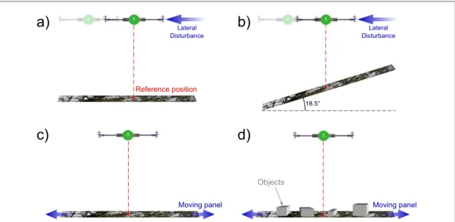
Figure 8summarizes the four scenarios used to show the visual stabilization capabilities of HyperRob.
Sections2and3presented the visual sensor and the algorithm we implemented on HyperRob. It is a twin-rotor robot tethered at the tip of a rotating arm. The robot was free to rotate around its roll axis and could therefore make the arm rotate around its vertical axis (the azimuth). The robot therefore travelled along a circular path with a radius of curvature equal to the length of the arm (1 m). Figure 9 shows the robot equipped with active CurvACE placed on the experi-mental testbench.
This section introduces HyperRob and we will see in section5.2.1that the robot will be able to stay at its initial position due to the vibrating active CurvACE estimating its linear speed and position, assuming that its gaze is stabilized.
4.1. Gaze stabilization
In order to determine the robot’s speed and position accurately, the gaze direction should be orthogonal to the terrain. But as a simplification, we chose to align it with the vertical, assuming that the ground is mostly horizontal. Therefore, the eye has to compensate for the robot’s roll angle. To this end, the eye is decoupled from the robot’s body by means of a servo motor with a rotational axis aligned with the robot’s roll axis. The gaze control system, composed of an inertial feedfor-ward control, makes the eye looking always in a perpendicular direction to the movement during flight (figure10). The rotational component introduced by the rotating arm supporting the robot can be neglected in this study.
Figure 8. The robot HyperRob flies over a textured panel and stays automatically at a programmed reference position despite lateral disturbance (a and b) , changes in the ground height (b), movement of the ground (c), or small relief introduced by several objects placed onto the ground (d).
4.2. Details of the robot HyperRob
HyperRob is an aerial robot with two propellers and a carbon fiber frame, which includes two DC motors. Each motor transmits its power to the corresponding propeller (diameter 13 cm) via a 8 cm long steel shaft rotating on microball bearings in the hollow beam, ending in a crown gear (with a reduction ratio of 1/5). Two Hall effect sensors were used to measure the rotational speed of each propeller, and hence its thrust, via four magnets glued to each crown gear. Based on the differential thrust setpoints adopted, HyperRob
can control its attitude around the roll axis, which is sensed by a six-axis inertial sensor (here an InvenSense MPU 6000). The robot’s position in the azimuthal plane is controlled by adjusting the roll angle. In the robot, where only the roll rotation is free, only one axis of the accelerometer and one axis of the rate gyro are used. As shown in figure 11, active CurvACE is mounted on a fast micro-servomotor (MKS DS 92A+) which makes it possible to control the gaze with great accuracy (0.1°) and fast dynamics (60° within 70 ms, i.e. 860°/s). This configuration enables the visual
Figure 9. Experimental setup of the robot HyperRob (a) Active CurvACE with a ROI (inset) composed of only 40 artificial ommatidia (8 × 5), each photosensor is composed of one pixel and one lens. FOV covers about33.6°by20.2 . (Picture provided by courtesy of P.° Psaïla) (b) The robot HyperRob and its active CurvACE sensor. (c) The complete setup consisted of a twin-propeller robot attached to the tip of a rotating arm. The robot was free to rotate around its roll axis. Arm rotations around the azimuth were perceived by the robot as lateral displacements.
Figure 10. Decoupled eye on the roll axis. Three examples of gaze stabilization. Despite the strong roll disturbances applied by hand to the body, the gaze orientation was kept vertically aligned by the mechanical decoupling provided by a fast servomotor between the robot’s body and the visual sensor. It can be clearly seen from the sequence of pictures that the yellow line remained horizontal regardless of the robot’s roll angle (red line).
sensor to be mechanically decoupled from the body (see section4.1). The robot is fully autonomous in terms of its computational resources and its power supply (both of which are provided onboard). The robot alone weighs about 145 g and the robot plus the arm weigh about 390 g.
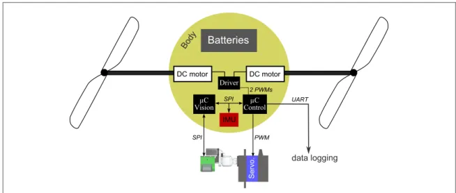
All the computational resources required for the visual processing and the autopilot are implemented on two power lean micro-controllers embedded onboard the robot. The first micro-controller (Micro-chip dsPIC 33FJ128GP802) deals with the visual pro-cessing, whereas the second one (Microchip dsPIC 33FJ128GP804) is responsible for stabilizing the robot. The two micro-controllers have a sampling fre-quency of 500 Hz. The robot’s hardware architecture is presented in detail in figure12.
The micro-controller (μC) Vision communicates with CurvACE via a serial peripheral interface (SPI)
bus and collects the pixel values of the ROI. The signal Sfused is computed and sent to the μC Control via
another SPI bus. The latter completes the computa-tion of the posicomputa-tionX¯ and the speedV¯x. This solution was chosen in order to keep the number of data sent via the SPI bus to a minimum. The μC Control esti-mates the robot’s attitude on the roll axis via a reduced complementary filter (inspired by [43]) and controls the robot’s linear position on the basis of the two visual measurements (X and Vxsee figure13). The μC
Con-trol then sends the propeller speed setpoints to a cus-tom-made driver controlling the rotational speed of each propeller in a closed-loop mode.
4.3. Control
Assuming the robot to be a rigid body and simplifying the dynamic model for a quad-rotor presented in [44] in the case of a single roll axis, the robot’s dynamics
Figure 11. Robot description (a) HyperRob mounted at the tip of the arm, leaving it free to rotate around the roll axis and move along a circular path in the azimuthal plane. (b) Schematic view of the robot. Four actuators were mounted onboard the robot: two DC motors driving the propeller’s rotation are set in the carbon fiber body, one servomotor is used to stabilize the gaze and one stepper motor is used to produce the eye tremor (vibration). (c) CAD view showing the robot equipped with its visual sensor with a FOV of
°
33.6 by20.2 .°ωr1andωr2are the two propellers’ rotation speeds,θris the robot’s roll angle, andθeris the eye-in-robot angle.
can be written as follows: θ θ Ω Ω Γ δ = = − = = θ=
( )
X V V T m sin l I ˙ ˙ ˙ ˙ 2 (12) x x nom r r r r ⎧ ⎨ ⎪ ⎪ ⎪ ⎩ ⎪ ⎪ ⎪where X is the robot’s lateral position, Vxis its lateral
speed,θris the roll angle,Ωris the rotational roll speed,
l is the robot’s half span, I is the moment of inertia, δ is the differential thrust, and Tnomis the nominal thrust.
δ ω ω δ δ = − = − = + = − ⋆ ⋆
(
)
T T c T T T T 2 (13) T r r nom nom 1 2 21 22 1 2 ⎧ ⎨ ⎪⎪ ⎩ ⎪⎪ ω δ ω δ ⇔ = + = − ⋆ ⋆(
)
(
)
T C T C r nom T r nom T 1 2 ⎧ ⎨ ⎪ ⎪⎪ ⎩ ⎪ ⎪ ⎪where cTis the thrust coefficient, andωr1andωr2are
the right and left propeller speeds, respectively, and
Figure 12. Electronic architecture. The autopilot’s electronics board is composed of two micro-controllers. The first one is involved in the visual processing algorithm (dsPIC33FJ128GP802) and the second one (dsPIC33FJ128GP804) controls the robot’s roll and its linear position. The micro-controller denoted μC Vision communicates with CurvACE and receives the digitized pixel output values via a SPI bus. The second micro-controller, denoted μC Control (dsPIC33FJ128GP804), receives the visual sensor’s output data from the micro-controller μC Vision via an additional SPI bus. The μC Control then sends the propellers’ setpoints to a custom-made driver including a closed-loop control of the rotational speed of each propeller.
Figure 13. Description of the control loops. The robot’s control system consists mainly of four nested feedback loops: one for the lateral position, one for the lateral speed VX, one for the roll angleθr, and one for the rotational roll speedΩr. The propellers’ speeds
ωr1,2are controlled via an additional local feedback loop. All the controllers are detailed in table1. Two Hall effect sensors are used to
measure the propeller speed used in the feedback loop controlling the effective thrust. The inertial sensors give a biased rotational speedΩ¯rand the accelerationA¯cc. The active CurvACE sensor produces two visual measurements, corresponding to the robot’s
δ=f ( )s δ⋆
prop , where fprop(s) and δ⋆correspond to the
closed-loop transfer function of the propellers’ speed and the differential thrust reference, respectively.
As described in figure13, the autopilot controlling both the robot’s roll and its position is composed of four nested feedback loops:
• the first feedback loop controls the robot’s rota-tional speed by directly adjusting the differential thrust, and hence the roll torque.
• the second feedback loop yields setpoints on the previous one for tracking the robot’s reference roll angle.
• the third feedback loop adjusts the robot’s linear speed by providing roll angle setpoints.
• the fourth feedback loop controls the robot’s linear position and yields the reference speed.
In the first and second feedback loops, the roll angle’s estimation is obtained by means of a reduced version of a complementary filter described in ([43]). In the case of HyperRob, since only a 1D filtering method is required, the attitude estimator becomes:
θ θ θ Ω Ω θ Ω θ θ = = − − = − = + −
(
)
(
)
arcsin Y g b k b k ¯ ˆ˙ ¯ ˆ ˆ ¯ ˆ ˆ˙ ˆ ¯ ˆ (14) r acc b r r r r r r a r r ⎧ ⎨ ⎪ ⎪ ⎪⎪ ⎩ ⎪ ⎪ ⎪⎪ ⎛ ⎝ ⎜ ⎞⎠⎟whereθ¯r is the roll angle calculated from the
accel-erometer measurement Yacc,bˆ is the estimated rate
gyro’s bias,Ω¯ris the rate gyro’s output measurement,
θˆr is the estimated roll angle, andΩˆr is the unbiased
rotational speed. Here ka and kb are positive gains
which were selected so as to obtain a convergence time of 3 s and 30 s for the estimated angle and the estimated rate gyro’s bias, respectively.
The complementary filter therefore yields the values of the rate gyro bias, the unbiased roll rotational speed, and the roll angle.
5. Application to short-range odometry,
visual stabilization, and tracking
In the various experiments performed in this study, a serial communication with a ground station was used to record the data provided by the robot. A VICON motion tracking system was run at the same time to obtain the ground-truth data. A textured panel was placed 39 cm below the robot. During the experiment involving the translation of the panel, as the sensor can only sense the movement along one direction and the robot travels along a circular path, the data were projected in order to obtain a comparable dataset.
Thus, at each time step, we projected the position vector into the robot frame and took only the tangential components of the displacement.
In this section, we report on several experiments which were carried out in order to test the robot’s cap-ability to perform various tasks. In all these experi-ments, thanks to the efficient gaze control system compensating for the robot’s roll, the visually con-trolled robot experienced a quasi-translational OF eli-cited by the perturbations applied either to the robot itself or to the textured panel. In the first experiment, the sensor played the role of an odometer. The robot achieved accurate hovering performances despite the lateral disturbances, as well as an efficient tracking capability. All these experiments confirmed that the robot was able to perform robust short-range visual odometry, i.e., to estimate its linear position before returning automatically to an arbitrary reference posi-tion adopted.
5.1. Short-range visual odometry
The fused visual output signal Sfusedprovided by the active
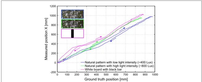
CurvACE depends on the visual environment: if there are no contrasts, the sensor will not detect any visual cues and will therefore not be able to specify the robot’s position accurately. The richer the visual environment is (in terms of contrasts), the better the position measurement. In order to compare the output of the sensor with the ground-truth measurements, three experiments were conducted under different visual conditions.
In these experiments, the robot was moved manually over two different panels under two different ambient lighting conditions from right to left and back to the initial position with its gaze stabilization activated. The results obtained, which are presented in figure14, are quite simi-lar for each trip, giving a maximum error of 174 mm. Figure14shows that the output in response to a textured panel and one composed of a single 5 cm wide black bar was similar. Therefore, assuming the distance to the ground to be known, the active CurvACE was able to serve as a visual odometer by measuring the robot’s position accurately in the neighbourhood of its initial position. 5.2. Lateral disturbance rejection
5.2.1. Above a horizontal textured panel
Lateral disturbances were applied by pushing the arm in both directions, simulating gusts of wind. In figure15, it can be seen that all lateral disturbances were completely rejected within about 5 s, including even those as large as 40 cm. The dynamics of the robot could be largely improved by using a robot with a higher thrust or a lighter arm in order to reduce the oscillation. Figures15(b) and (c) show that the robot was always able to return to its initial position. With its active eye, the robot can compensate for lateral disturbance as large as 359 mm applied to its reference position with a maximum error of only 25 mm, i.e., 3% of the flown distance. This error is presumably due
to the selection process, which does not ensure the selection of the same features in the outward path and on the way back to the reference position; or maybe the assumption of a linear approximation of the inverse tangent function does not hold entirely within the entire FOV. As a consequence, thanks to the active visual sensor and its capability to measure the angular position of contrasting features, the robot HyperRob is highly sensitive to any motion and thus can compensate for very slow perturbation, ranging here from 0 to 391 mm. s−1
. 5.2.2. Above an evenly sloping ground
In the previous experiment, it was assumed that the ground height must be known to be able to use the conversion gain in the fused output signal Sfused. The
same experiment was repeated here above a sloping
ground (see figure16). The robot’s height increased sharply in comparison with the calibration height. The robot’s height varied in the range of +/−74 mm and starts with an offset of +96 mm compared to the calibration height. As shown in figure 16(b), the estimation of the traveled distance was always under-estimated because the robot was always higher than the calibration height. However, the robot was still able to return to its starting position with a maximum error of only 45 mm (timet= 36. 5 s) for a distur-bance of 210 mm (i.e., 10.5% of the flown distance). 5.3. Tracking
The robot’s tracking performances are presented in this subsection. Three different tracking tasks were tested:
Figure 14. Robustness of the sensor. Comparison between the active CurvACE sensor’s measurements and the ground-truth position given by the VICON system when the robot made a lateral movement and returned to its initial position. The sensor’s output remained fairly stable regardless the lighting conditions and structure of the pattern, giving a standard error ranging from 2.3 to 7.8% (Deviation= max xStd( )error i−(ymin x−x( )i)
i i ).
Figure 15. Lateral disturbance rejection over a naturally textured panel (a) Robot’s position (in blue) superimposed on the panel’s position (in red), both measured by the VICON system. The robot rejected the series of disturbances and returned to its initial position with a maximum error of 25 mm in less than 5 s. (b) The visual errors measured by the robot (red) and the VICON (blue) were very similar. With large disturbances, small errors occurred in the visual estimation of the robot’s position without noticeably affecting the robot’s capability to return automatically to its starting position. (c) Ground-truth measurement of the robot speed error (red curve) and the visual speed error (blue curve) measured by the robot due to active CurvACE. These two curves show that the robot was able to compensate for maximum lateral speed of 391 mm. s−1.
• tracking a moving textured panel (see section5.3.1).
• tracking a moving textured panel with 3D objects placed on it (see section5.3.2).
• tracking moving hands perceived above a stationary textured panel (see section5.3.3).
5.3.1. Panel Tracking
In this experiment, the panel was moved manually and the robot’s reference position setpointX was kept at⋆ zero. The robot faithfully followed the movements imposed on the panel. The few oscillations which occurred were mainly due to the robot’s dynamics rather than to visual measurement errors. Each of the panel’s movements was clearly detected, as shown in figure 17(b), although a proportional error in the measurements was sometimes observed, as explained above.
5.3.2. Tracking a moving rugged ground
In the second test, some objects were placed on the previously used panel to create an uneven surface. The robot’s performances on this new surface were similar
to those observed on the flat one, as depicted in figure 18. The visual error was not as accurately measured as previously over the flat terrain because of the changes in the height of the ground. But the robot’s position in the steady state was very similar to that of the panel. The maximum steady-state error att=19 s was only 32 mm .
5.3.3. Toward figure-ground discrimination: hand tracking
The last experiment consisted of placing two moving hands between the robot and the panel. Markers were also placed on one of the hands in order to compare the hand and robot positions: the results of this experiment are presented in figure19. As shown in the video in the Supplementary Data and in figure19, the robot faithfully followed the hands when they were moving together in the same direction. By comparing the robot position error seen by the active CurvACE with the ground-truth error, it was established that the robot tracked the moving hands accurately with a maximum estimation error of 129 mm.
Our visual algorithm selects the greatest contrasts in order to determine its linear position with respect to an arbitrary reference position. Therefore, when the
Figure 16. Disturbances above a sloping ground (a) Picture of the robot above the sloping ground at an angle of18.5 with respect to° the horizontal. In the case of a300mm horizontal displacement, the height increased by100mm. definitions of the terms height and shift are also displayed. The robot is subjected to a series of disturbances with a maximum amplitude of200mm. (b) Horizontal shift measured by the sensor (blue) and the theoretical one calculated from VICON data (red). (c) Vertical distance from the robot to the panel in comparison with the calibration height of 390 mm.
Figure 17. Tracking a naturally textured panel. When the textured panel was moved manually below the robot, HyperRob automatically followed the movement imposed by the panel. (a) Tracking of the panel by the robot. The red line corresponds to the panel’s position and the blue line to the robot’s position, both measured by the VICON system. (b) Comparison between the position measurement error given by the visual system (in blue) and the ground-truth data (in red) given by the VICON system. The results show that the robot tracked the moving panel accurately with a maximal position estimation error of 39 mm for a panel translation of 150 mm.
Figure 18. Tracking a rugged ground with height variations formed by objects A rugged surface including several objects was moved below the robot, which had to follow the movements imposed on the ground. (a) Picture showing the robot’s visual environment during the test. (b) Tracking of the panel by the robot. The red line corresponds to the panel position and the blue line to the robot’s position, both measured by the VICON system. (c) Comparison between the position measurement error given by the visual system (in blue) and the ground-truth error (in red) given by the VICON measurements.
hands were moving above the panel, some stronger contrasts than those of the hands were detected by the visual sensor, which decreased the accuracy of its tracking performances. However, this experiment showed that the robot is still able to track an object when a non-uniform background is moving differ-ently, without having to change the control strategy or the visual algorithm. The robot simply continues to track the objects featuring the greatest contrasts.
6. Conclusion
In this paper, we describe the development and the performances of a vibrating small-scale cylindrical curved compound eye, named active CurvACE. The active process referred to here means that miniature periodic movements have been added in order to improve CurvACE’s spatial resolution in terms of the localization of visual objects encountered in the surroundings. By imposing oscillatory movements (with a frequency of 50 Hz) with an amplitude of a few degrees (5 ) on this artificial compound eye, it was° endowed with hyperacuity, i.e., the ability to locate an object with much greater accuracy than that achieved so far because of the restrictions imposed by the interommatidial angle. Hyperacuity was achieved here by 35 LPUs applying the same local visual processing algorithm across an ROI of active CurvACE consisting of 8 × 5 artificial ommatidia. The novel sensory fusion algorithm used for this purpose, which was based on the selection of the 10 highest contrasts, enables the active eye (2D-FOV:32°by20°) to assess its displace-ment with respect to a textured environdisplace-ment. We even established that this new visual processing algorithm is
Figure 19. Tracking moving hands above a textured panel In this experiment, the textured panel was kept stationary while two hands were moving horizontally together between the robot and the panel. (a) Picture of the hands during the experiment conducted with VICON. Markers are only required to monitor the hands’ position. In the video provided in the Supplementary Data, we showed that the robot’s performances are similar without those markers. (b) Plots of the textured panel’s position (red), the robot’s position (blue), and the hands’ position (green), all measured by VICON. The robot followed the moving hands faithfully over the ground. (c) Comparison between the error measured by the eye (blue), and the ground-truth error provided by the VICON system (green). The latter is equal to the (Hand_Position)-(Robot_Position).
Table 1. Controllers’ parameters.
Controller
Transfer
Functions Parameters Value Position controller Kx Kx=0.6s−1
Lateral speed controller K .V τ +Vss 1 KV= 0.7
τ =V 0.71
Roll controller Kθ Kθ=0.6 Robot rot. speed
controller
Ω τ +Ω
K . ss 1 KΩ=0.06
τ =Ω 0.45
Motor rot. speed controller
ω τ +ω
K . ss 1 Kv= 0.9
τ =ω 0.05
a first step toward endowing robots with the ability to perform figure/ground discrimination tasks. By apply-ing miniature movements to a stand-alone artificial compound eye, we developed a visual odometer yielding a standard error of 7.8% when it was subjected to quasi-translational movements of 1 m. Moreover, active CurvACE enabled a robot to hover and return to a position after perturbations with a maximal error of 2.5 cm for experiments based on a flat terrain, which is state-of-the-art performance in aerial robotics (see table2), although our study is about a tethered robot flying indoors.
All the solutions adopted in this study in terms of practical hardware and computational resources are perfectly compatible with the stringent specifications applying to low-power, small-sized, low-cost micro-aerial vehicles (MAVs). Indeed, thanks to active Cur-vACE, we achieved very accurate hovering flight with few computational resources (only two 16 bit micro-controller and few pixels (only 8 × 5). However, the 1D visual scanning presented here should be extended to a 2D scanning so as to enable free flight, which, however, would require a completely new mechanical design. In addition, the architecture of the 2D visual processing algorithm will have to be revised to make it compatible with low computational overheads. It is worth noting that the gaze stabilization reflex imple-mented onboard the present robot requires very few computational resources and allows CurvACE to pro-cess visual information resulting from purely transla-tional movements. In addition, recent robotic studies have shown that gaze stabilization can be a useful means of achieving automatic heading [45] and vision-based hovering [46]. The MAVs of the future (e.g., [47]) will certainly require very few
computational resources to perform demanding tasks such as obstacle avoidance, visual stabilization, target tracking in cluttered environments, and autonomous navigation. Developing airborne vehicles capable of performing these highly demanding tasks will cer-tainly involve the use of the latest cutting-edge tech-nologies and bio-inspired approaches of the kind used here.
Acknowledgments
The authors would like to thank Marc Boyron and Julien Diperi for the robot and the testbench realization; Nicolas Franceschini for helping in the design of the robot, Franck Ruffier for the fruitful discussions and the help implementing the flying arena. We would like to thank the referees for carefully reading our manuscript and for giving constructive feedback which improved significantly the quality of the paper. We also acknowl-edge the financial support of the Future and Emerging Technologies (FET) program within the Seventh Frame-work Programme for Research of the European Com-mission, under FET-Open Grant 237940. This work was supported by CNRS, Aix-Marseille University, Prov-ence-Alpes-Cote d’Azur region, and the French National Research Agency (ANR) with the EVA, IRIS, and Equipex/Robotex projects (EVA project and IRIS project under ANR grants’ number ANR608-CORD-007-04, and ANR-12-INSE- 0009, respectively).
References
[1] Westheimer G 1975 Editorial: visual acuity and hyperacuity Investigative Ophthalmology & Visual Science 14 570–2 [2] Westheimer G 2009 Hyperacuity Encyclopedia of Neuroscience
5 45–50 Sensor σ σ = = 84 ? y z ≈0.3 Yang et al [28] Firefly MV 680× 480 σ σ == 38.8 5.7 x y z , 1
Shen et al [22] 2 uEye 1220SE 752 × 480 σ
σ σ = = = 31.3 52.9 27.2 x y z 0.9
[3] Floreano D et al 2013 Miniature curved artificial compound eyes Proc. Nat. Acad. Sci. USA110 9267–72
[4] Viollet S et al 2014 Hardware architecture and cutting-edge assembly process of a tiny curved compound eye Sensors14 21702–21
[5] Rolfs M 2009 Microsaccades: small steps on a long way Vis. Res.49 2415–41
[6] Sandeman D C 1978 Eye-scanning during walking in the crab leptograpsus variegatus J. Comp. Physiol.124 249–57
[7] Land M F 1969 Movements of the retinae of jumping spiders (salticidae: Dendryphantinae) in response to visual stimuli J. Exper. Bio. 51 471–93
[8] Land M 1982 Scanning eye movements in a heteropod mollusc J. Exper. Bio. 96 427–30
[9] Kaps F and Schmid A 1996 Mechanism and possible beha-vioural relevance of retinal movements in the ctenid spider cupiennius salei J. Exper. Bio. 199 2451–8
[10] Viollet S 2014 Vibrating makes for better seeing: from the fly’s micro eye movements to hyperacute visual sensors Frontiers Bioengin. Biotech.2
[11] Mura F and Franceschini N 1996 Obstacle avoidance in a terrestrial mobile robot provided with a scanning retina Proc. 1996 IEEE Intel. Veh. Symp. (19–20 Sept 1996) pp 47–52 [12] Viollet S and Franceschini N 2010 A hyperacute optical
position sensor based on biomimetic retinal micro-scanning Sensors and Actuators A: Physical160 60–68
[13] Kerhuel L, Viollet S and Franceschini N 2012 The vodka sensor: a bio-inspired hyperacute optical position sensing device Sensors J. IEEE12 315–24
[14] Juston R, Kerhuel L, Franceschini N and Viollet S 2014 Hyperacute edge and bar detection in a bioinspired optical position sensing device Mechatronics, IEEE/ASME Transac-tions on19 1025–34
[15] Wright C H G and Barrett S F 2013 Chapter 1—biomimetic vision sensors Engineered Biomimicry ed A Lakhtakia and R J Mart-Palma (Boston: Elsevier) pp 1–36
[16] Benson J B, Luke G P, Wright C and Barrett S F 2009 Pre-blurred spatial sampling can lead to hyperacuity Digital Signal Processing Workshop and 5th IEEE Signal Processing Education Workshop 2009. DSP/SPE 2009. IEEE 13th p 570–575 [17] Luke G P, Wright C H G and Barrett S F 2012 A multiaperture
bioinspired sensor with hyperacuity Sensors J. IEEE12 308–14
[18] Riley D T, Harmann W M, Barrett S F and Wright C H G 2008 Musca domestica inspired machine vision sensor with hypera-cuity Bioinspiration & Biomimetics 3 026003
[19] Brückner A, Duparré J, Bräuer A and Tünnermann A 2006 Artificial compound eye applying hyperacuity Optics Express
14 12076–84
[20] Wilcox M J and Thelen D C Jr 1999 A retina with parallel input and pulsed output, extracting high-resolution information Neural Networks, IEEE Trans.10 574–83
[21] Davis J D, Barrett S F, Wright C H G and Wilcox M 2009 A bio-inspired apposition compound eye machine vision sensor system Bioinspiration & Biomimetics 4 046002
[22] Shen S, Mulgaonkar Y, Michael N and Kumar V 2013 Vision-based state estimation for autonomous rotorcraft mavs in complex environments 2013 IEEE Int. Conf. Robotics Automa-tion (ICRA) (Karlsruhe, Germany) p 1758–1764
[23] Forster C, Pizzoli M and Scaramuzza D 2014 SVO: Fast semi-direct monocular visual odometry 2014 IEEE Int. Conf. Robotics Automation (ICRA) pp 15–22
[24] Kendoul F, Nonami K, Fantoni I and Lozano R 2009 An adaptive vision-based autopilot for mini flying machines guidance, navigation and control Auton. Robots27 165–88
[25] Engel J, Sturm J and Cremers D 2012 Accurate figure flying with a quadrocopter using onboard visual and inertial sensing Workshop on Visual Control of Mobile Robotos (ViCoMoR) at the IEEE/RSJ Int. Conf. Intelligent Robots Sys (Vilamoura, Protugal) vol 320 240
[26] Mkrtchyan A A, Schultz R R and Semke W H 2009 Vision-based autopilot implementation using a quadrotor helicopter AIAA Infotech@ Aerospace Conf. (Seattle, Washington) 1831 [27] Zhang T, Kang Y, Achtelik M, Kühnlenz K and Buss M 2009
Autonomous hovering of a vision/imu guided quadrotor Int. Conf. Mechatronics Automation (ICRA) (Changchun, China)
pp 2870–2875
[28] Yang S, Scherer S A and Zell A 2013 An onboard monocular vision system for autonomous takeoff, hovering and landing of a micro aerial vehicle J. Intel. Robotic Sys.69 499–515
[29] Bosnak M, Matko D and Blazic S 2012 Quadrocopter hovering using position-estimation information from inertial sensors and a high-delay video system J. Intel. Robotic Sys.67 43–60
[30] Gomez-Balderas J E, Salazar S, Guerrero J A and Lozano R 2014 Vision-based autonomous hovering for a miniature quad-rotor Robotica32 43–61
[31] Lim H, Lee H and Kim H J 2012 Onboard flight control of a micro quadrotor using single strapdown optical flow sensor 2012 IEEE/RSJ Int. Conf. Intel. Robots Sys. (IROS) (Vilamoura, Algarve, Portugal)pp 495–500
[32] Herissé B, Hamel T, Mahony R and Russotto F-X 2012 Landing a vtol unmanned aerial vehicle on a moving platform using optical flow IEEE Trans. Robotics28 77–89
[33] Ruffier F and Franceschini N 2014 Optic flow regulation in unsteady environments: a tethered mav achieves terrain following and targeted landing over a moving platform J. Intel. Robotic Sys.pp 1–19
[34] Carrillo L R G, Flores G, Sanahuja G and Lozano R 2012 Quad-rotor switching control: an application for the task of path following American Control Conf. (ACC) (Fairmont Queen Elizabeth, Montréal, Canada) p 4637–4642
[35] Honegger D, Meier L, Tanskanen P and Pollefeys M 2013 An open source and open hardware embedded metric optical flow cmos camera for indoor and outdoor applications 2013 IEEE Int. Conf. Robotics Automation (ICRA) pp 1736–1741 IEEE [36] Bristeau P-J et al 2011 The navigation and control technology
inside the ar. drone micro uav 18th IFAC world congress vol 18 pp 1477–1484
[37] Hengstenberg R 1972 Eye movements in the housefly musca domestica Information Processing in the Visual Systems of Anthropods ed R Wehner (Berlin Heidelberg: Springer)
p 93–96
[38] Land M F and Nilsson D-E 2012 Animal Eyes (Oxford Animal Biology Series) 2nd edn (Oxford: Oxford University Press) [39] Stavenga D G 2003 Angular and spectral sensitivity of fly
photoreceptors. i. integrated facet lens and rhabdomere optics J. Comp. Physiol. A 189 1–17
[40] Horridge G A 1977 The compound eye of insects Sci. Amer.
237 108–20
[41] Carpenter R H S 1988 Movements of the eyes (London: Pion Limited)
[42] Juston R and Viollet S 2012 A miniature bio-inspired position sensing device for the control of micro-aerial robots Intelligent Robots and Systems (IROS) 2012 IEEE/RSJ Int. Conf.
p 1118–1124
[43] Mahony R, Hamel T and Pflimlin J-M 2008 Nonlinear complementary filters on the special orthogonal group IEEE Trans. Automatic Control5 1203–18
[44] Bouabdallah S, Murrieri P and Siegwart R 2004 Design and control of an indoor micro quadrotor Int. Conf. Robotics Automation (ICRA) vol 5 4393–8
[45] Kerhuel L, Viollet S and Franceschini N 2010 Steering by gazing: An efficient biomimetic control strategy for visually guided micro aerial vehicles IEEE Trans. Robotics26 307–19
[46] Manecy A, Marchand N and Viollet S 2014 Hovering by gazing: a novel strategy for implementing saccadic flight-based navigation in gps-denied environments Int. J. Adv. Robotic Sys.11(66)
[47] Ma K Y, Chirarattananon P, Fuller S B and Wood R J 2013 Controlled flight of a biologically inspired, insect-scale robot Science340 603–7