HAL Id: hal-02333641
https://hal.archives-ouvertes.fr/hal-02333641
Submitted on 11 Nov 2020
HAL is a multi-disciplinary open access
archive for the deposit and dissemination of
sci-entific research documents, whether they are
pub-lished or not. The documents may come from
teaching and research institutions in France or
abroad, or from public or private research centers.
L’archive ouverte pluridisciplinaire HAL, est
destinée au dépôt et à la diffusion de documents
scientifiques de niveau recherche, publiés ou non,
émanant des établissements d’enseignement et de
recherche français ou étrangers, des laboratoires
publics ou privés.
The STAGGER-grid: A grid of 3D stellar atmosphere
models
A. Chiavassa, L. Casagrande, R. Collet, Z. Magic, L. Bigot, Frédéric
Thévenin, M. Asplund
To cite this version:
A. Chiavassa, L. Casagrande, R. Collet, Z. Magic, L. Bigot, et al.. The STAGGER-grid: A grid of
3D stellar atmosphere models: V. Synthetic stellar spectra and broad-band photometry. Astronomy
and Astrophysics - A&A, EDP Sciences, 2018, 611, pp.A11. �10.1051/0004-6361/201732147�.
�hal-02333641�
3 Stellar Astrophysics Centre, Department of Physics and Astronomy, Aarhus University, Ny Munkegade 120, 8000 Aarhus C,
Denmark
4 Niels Bohr Institute, University of Copenhagen, Juliane Maries Vej 30, 2100 Copenhagen, Denmark
5 Centre for Star and Planet Formation, Natural History Museum of Denmark, University of Copenhagen, Øster Voldgade 5-7,
1350 Copenhagen, Denmark
Received 20 October 2017 / Accepted 4 January 2018
ABSTRACT
Context. The surface structures and dynamics of cool stars are characterised by the presence of convective motions and turbulent flows which shape the emergent spectrum.
Aims. We used realistic three-dimensional (3D) radiative hydrodynamical simulations from the STAGGER-grid to calculate synthetic spectra with the radiative transfer code OPTIM3D for stars with different stellar parameters to predict photometric colours and convec-tive velocity shifts.
Methods. We calculated spectra from 1000 to 200 000 Å with a constant resolving power of λ/∆λ= 20 000 and from 8470 and 8710 Å (Gaia Radial Velocity Spectrometer – RVS – spectral range) with a constant resolving power of λ/∆λ= 300 000.
Results. We used synthetic spectra to compute theoretical colours in the Johnson-Cousins U BV(RI)C, SDSS, 2MASS, Gaia,
SkyMap-per, Strömgren systems, and HST-WFC3. Our synthetic magnitudes are compared with those obtained using 1D hydrostatic models. We showed that 1D versus 3D differences are limited to a small percent except for the narrow filters that span the optical and UV region of the spectrum. In addition, we derived the effect of the convective velocity fields on selected Fe I lines. We found the overall convective shift for 3D simulations with respect to the reference 1D hydrostatic models, revealing line shifts of between −0.235 and +0.361 km s−1. We showed a net correlation of the convective shifts with the effective temperature: lower effective temperatures denote
redshifts and higher effective temperatures denote blueshifts. We conclude that the extraction of accurate radial velocities from RVS spectra need an appropriate wavelength correction from convection shifts.
Conclusions. The use of realistic 3D hydrodynamical stellar atmosphere simulations has a small but significant impact on the pre-dicted photometry compared with classical 1D hydrostatic models for late-type stars. We make all the spectra publicly available for the community through the POLLUX database.
Key words. stars: atmospheres – stars: fundamental parameters – techniques: photometric – techniques: radial velocities – hydrodynamics – radiative transfer
1. Introduction
The stellar atmosphere is the boundary to the opaque stellar interior, and serves as the link between observations and the models of stellar structure and evolution. The phenomena of stel-lar evolution manifest themselves in the stelstel-lar surface as changes in chemical composition and in fundamental stellar parameters such as radius, surface gravity, effective temperature, and lumi-nosity. The information we use to study distant stars comes from the flux they have emitted. However, the atmospheric layers where this flux forms is the transition region between convective and radiative regime. Thus, the surface structures and dynam-ics of cool stars are characterised by the presence of convective motions and turbulent flows. Convection manifests in the surface layers as a particular pattern of downflowing cooler plasma and
?Tables 5–8 are only available at the CDS and Table B.1
is also available at the CDS and via anonymous ftp to
cdsarc.u-strasbg.fr(130.79.128.5) or via
http://cdsarc.u-strasbg.fr/viz-bin/qcat?J/A+A/611/A11
bright areas where hot plasma rises (Nordlund et al. 2009). The size of granules depends on the stellar parameters of the star and, as a consequence, on the extension of their atmosphere (e.g. Magic et al. 2013). Eventually, the convection causes an inhomo-geneous stellar surface that changes with time. They affect the atmospheric stratification in the region where the flux forms and also affect the emergent spectral energy distribution (SED), with potential effects on the precise determinations of stellar parame-ters (e.g. Bigot et al. 2011;Creevey et al. 2012;Chiavassa et al. 2012), radial velocity (e.g. Bigot & Thévenin 2008;Chiavassa et al. 2011; Allende Prieto et al. 2013), chemical abundance (e.g. Asplund et al. 2005,2009;Caffau et al. 2011), photometric colours (Bonifacio et al. 2017), and on planet detection (Magic et al. 2015;Chiavassa et al. 2017).
Convection is a difficult process to understand because it is non-local, and 3D, and it involves non-linear interac-tions over many disparate length scales. In this context, the use of numerical 3D radiative hydrodynamical simulations of stellar convection is extremely important. In recent years, with
increased computational power, it has been possible to compute grids of 3D simulations that cover a substantial portion of the Hertzsprung–Russell diagram (Magic et al. 2013;Trampedach et al. 2013;Ludwig et al. 2009). With these tools it is possible to predict reliable synthetic spectra for several stellar types.
Photometric systems and filters are designed to be sensi-tive to temperature, gravity, and metal abundance indicators and thereby to complement spectroscopic determinations of the fundamental properties of stars. In addition, the integrated mag-nitudes and colours of stars can be used to infer the ages, metal-licities, and other properties of the underlying stellar populations (e.g. Casagrande & VandenBerg 2014). For these purposes, sev-eral broad-band, or intermediate- and/or narrow-band filters have been designed to probe different regions of stellar spectra sen-sitive to different atmospheric parameters (Bessell & Murphy 2012;Gunn et al. 2006;Cohen et al. 2003). Additionally, there are the photometric systems used by the Gaia mission.
Gaia(Gaia Collaboration 2016) is an astrometric, photo-metric, and spectroscopic spaceborne mission of a large part of the Milky Way. Apart from the astrometric instrument, Gaia carries on board two low-resolution spectrophotometers (Blue and Red Prism, BP/RP, Bailer-Jones et al. 2013) and the Radial Velocity Spectrometer (RVS; Katz et al. 2004). The photomet-ric instrument measures the SED over 120 pixels of all detected objects at the same angular resolution and at the same epoch as the astrometric observations. The BP operates in the range 3300–6800 Å, while the RP uses the range 6400–10 500 Å. The main aims of this instrument are to provide proper classifi-cations (e.g. distinguish between stars, galaxies, and quasars) and characterisations (e.g. reddenings and stellar parameters), and to enable chromatic corrections of the astrometric cen-troid data. Finally, the integral-field spectrograph RVS provides spectra between 8470 and 8710 Å at a spectral resolving power of ≈11 200. The RVS is expected to produce radial veloci-ties through Doppler-shift measurements; interstellar reddening, atmospheric parameters, and projected rotational velocities; and individual element abundances for some elements.
In this work, we calculated synthetic stellar spectra and photometry for broad-band and Gaia systems obtained using realistic 3D radiative hydrodynamical simulations of stellar con-vection from the STAGGER-grid. The predicted photometric 3D colours and the 3D spectra are publicly available for the community through the POLLUX database. The spectra corre-sponding to the Gaia RVS spectral range will be used for the calibration of the instrument to preserve the measured radial velocities from the convection shift (see forthcoming paper of GaiaDataRelease2/RVS).
2. Methods
2.1. Stellar model atmospheres
Magic et al. (2013) described the STAGGER-grid of realistic 3D radiative hydrodynamical simulations of stellar convec-tion for cool stars using the STAGGER-code (originally devel-oped by Nordlund & Galsgaard1, and continuously improved
over the years by its user community), a state-of-the-art (magneto)hydrodynamic code that solves the time-dependent hydrodynamic equations for mass-, momentum-, and energy-conservation, coupled with the 3D radiative transfer equation in order to account correctly for the interaction between the radiation field and the plasma. The code uses periodic boundary
1 http://www.astro.ku.dk/~kg/Papers/MHDcode.ps.gz
conditions horizontally and open boundaries vertically. At the bottom of the simulation, the inflows have a constant entropy. The outflows are not tightly constrained and are free to pass through the boundary. The code is based on a sixth-order explicit finite-difference scheme and a fifth-order interpolation. The con-sidered large number over wavelength points is merged into 12 opacity bins (Nordlund 1982; Skartlien 2000; Magic et al. 2013). STAGGERsimulations are based on a realistic equation of state that accounts for ionisation, recombination, and dissocia-tion (Mihalas et al. 1988); continuous absorption and scattering coefficients listed inHayek et al.(2010); and the line opacities listed inGustafsson et al.(2008). These are in turn based on the VALD-2 database (Stempels et al. 2001) of atomic lines and the SCAN-base (Jørgensen 1997) of molecular lines.
2.2. Three-dimensional radiative transfer
We used the 3D pure-LTE radiative transfer code OPTIM3D (Chiavassa et al. 2009) to compute synthetic spectrum from the snapshots of the radiative-hydrodynamical (RHD) simulations of the STAGGER-grid (see Fig. 1 in Magic et al. 2013). The code takes into account the Doppler shifts due to convective motions. The radiative transfer equation is solved monochromat-ically using pre-tabulated extinction coefficients as a function of temperature, density, and wavelength.
The lookup tables were computed for the same chemical compo-sitions as the RHD simulations using the same extensive atomic and molecular continuum and line opacity data as the latest gen-eration of MARCS models (Gustafsson et al. 2008) with the addition – with respect to Table 2 of Gustafsson’s paper – of the SiS molecule (Cami et al. 2009), which is particularly important for the far-infrared region of the spectrum. While the sources of line opacities used in the RHD simulations ofMagic et al.(2013) and in OPTIM3D are the same, the data for the continuum opac-ities are almost the same:Hayek et al.(2010) reported that the data used in RHD simulations are mostly identical to those used in the MARCS models, but include additional bound-free data from the Opacity Project and the Iron Project (Trampedach et al., priv. comm.) as well as some opacities of the second ionisation stage for many metals.
For the computation of the spectra from RHD simulations, the assumed microturbulence is equal to zero since the velocity fields inherent in RHD models are expected to self-consistently and adequately account for non-thermal Doppler broadening of spectral lines (Asplund 2000). The temperature and density ranges spanned by the tables are optimised for the values encoun-tered in the RHD simulations. The detailed methods used in the code are explained inChiavassa et al.(2009,2010). OPTIM3D has already been employed in synergy with the STAGGER simu-lations in several works (Chiavassa et al. 2010,2011,2012,2014a, 2015,2017;Magic et al. 2015) either concerning the extraction of synthetic spectra or interferometric observables.
2.3. One-dimensional radiative transfer
For all the following comparisons with 3D simulations, we used plane-parallel, hydrostatic, 1D atmosphere models computed with a similar physical treatment to the MARCS code and the same equation of state and opacities as in the individual 3D simulations (ATMO; Magic et al. 2013). Moreover, we used a 1D version of OPTIM3D, and the chemical compositions, the opacities, and numerics of the radiative transfer calculations for the emergent intensities are the same as used in the 1D and 3D approaches.
Fig. 1. Surface rendering for all the synthetic spectra com-puted for the 3D RHD simula-tions in Table B.1. The verti-cal bar on the right displays the colour scale for the emerging flux in erg s−1cm−2Å−1. For clarity,
the wavelength range has been reduced to 1000–25 000 Å.
Fig. 2.Synthetic spectra of the solar simulation in the spectral range 2000–25 000 Å and for the different µ= cos(θ) inclination angles used in the computation, where θ is the angle with respect to the line of sight (vertical axis).
3. Synthetic spectra from 0.1 to 20 µm
The STAGGER-grid includes 3D stellar atmosphere simulations with metallicities [Fe/H] =+0.5, 0.0, −0.5, −1.0, −2.0, −3.0, and −4.0; surface gravity log g between 1.5 and 5.0 in steps of 0.5 dex; and effective temperature Teff from 4000 to 7000 K
in steps of 500 K (Fig. 1 of Paper I). In this work we present the synthetic spectra computed for the STAGGER-grid for a total of 181 simulations (Table B.1). The spectra have been calculated with a constant resolving power of λ/∆λ = 20 000 (nλ= 105 767 wavelength points) from 1000 to 200 000 Å. OPTIM3D computes the emerging intensities for vertical rays cast through the computational box for all required wavelengths. The procedure is repeated after tilting the computational box by an angle θ with respect to the line of sight (vertical axis) and rotating it azimuthally by an angle φ. The final result is a spatially resolved intensity spectrum at different angles. In
addition, a temporal average is also performed. We performed the calculations for ten snapshots of the 3D RHD simula-tions of TableB.1, adequately spaced so as to capture several convective turnovers, for ten different inclination angles µ = cos(θ) = [1.00, 0.90, 0.80, 0.70, 0.50, 0.30, 0.20, 0.10, 0.05, 0.01] (see Fig. 4), and four φ-angles [0◦, 90◦, 180◦, 270◦]. The
strongest decline in the limb darkening is usually found towards the limb; therefore, we decided to resolve with more µ-angles at the limb instead of having an equidistant scale in µ. We tested the discrepancy between the temporal average using a large number of snapshots (e.g. 20) and using only 10 snapshots is lower than 0.3%. The number of ten snapshots was chosen because it represents the best compromise in terms of computational time and accuracy among the whole set of stellar parameters. All things considered, we computed 400 spectra in the range 1000–200 000 Å for every simulation.
Figure1 displays the set of all synthetic spectra computed. We determined the Teff from the integration of the SED of the
spectra from 0.1 to 20 µm. The effective temperature has been computed using Stefan–Boltzmann law as
Teff spectra= ("Z λ2 λ1 f(λ) dλ # /σ )0.25 , (1)
where λ1 = 1010Å and λ2= 199 960 Å, f (λ) is the synthetic
flux, and σ is the Stefan–Boltzmann constant. The values of the effective temperature are listed in TableB.1.
Figure 1 shows that increasing Teff returns higher radiated
energy per surface area and the peak of the radiation curve moves to shorter wavelengths, as expected by Planck law. Pereira et al. (2013) provided excellent agreement of their 3D solar simulation of the STAGGER-grid with the continuum obser-vation of the Sun. As they did, we used the Kurucz (2005) irradiance2and normalised flux atlases for the Sun between 3000 and 10 000 Å and found a good agreement (Fig. 3), reinforc-ing the view that the simulation of thermodynamic structure
Fig. 3.Comparison of the solar simulation (black) with the observed flux of the Sun (red, Kurucz 2005). The solar irradiance is con-verted to flux at the solar surface using the multiplicative factor of [(1AU) /R ]2 = 46 202. For clarity, the spectra have been resampled to
a lower spectral resolution with fewer frequency points (nλ= 2115).
and post-processing detailed radiative transfer are realistic. This conclusion was also reported byHayek et al.(2012), who deter-mined that the numerical resolution of the STAGGER3D RHD models and the spectral resolution for the flux computations are sufficient to predict realistic observables. In particular, some of the RHD simulations presented in this work and for a limited spectral region between 2000 and 10 000 Å have been used in Magic et al.(2015) to provide appropriate coefficients for various bi-parametric and non-linear limb darkening laws.
4. Photometric synthetic observables
Photometric systems and filters are designed to probe funda-mental physical parameters, such as the effective temperature, surface gravity, and metallicity of stars. Colour and magni-tude relations are used for a variety of purposes: interpreting the observed distribution of stars in colour–colour and colour– magnitude diagrams, deriving distances to stars and star clusters, and testing stellar evolutionary theory by comparing with obser-vations to name just a few. Thus, it is important to have realistic model fluxes to generate colours which match the observed values. In addition to synthetic model fluxes, details on the photometric standardisation are also a part of this quest.
In essence, photometry condenses the information encoded in a spectrum f (λ) over a system response function T (λ), i.e. R
f(λ) T (λ) dλ. Each existing photometric system then varies in the details. Most notably, T (λ) will depend on the filter under consideration and the response function of the detec-tor. This means that a distinction must be made between photo-counting and energy-integration detectors, meaning that a measurement of energy R f(λ) T (λ) dλ will correspond to (hc)−1R f(λ) λT (λ) dλ photons (see e.g.Bessell 2000). Another aspect that often varies among different photometric systems is how their standardisation (zero-point and absolute calibra-tion) is achieved. Here, for all systems but Gaia we adopted the exact same procedure as used byCasagrande & VandenBerg (2014), where details on the adopted filter transmission curves, the photo-counting and energy-integration formalism, and zero-points and absolute calibration can be found3. We computed
3 The only difference with respect toCasagrande & VandenBerg(2014)
is that here we have adopted MBol = 4.74.
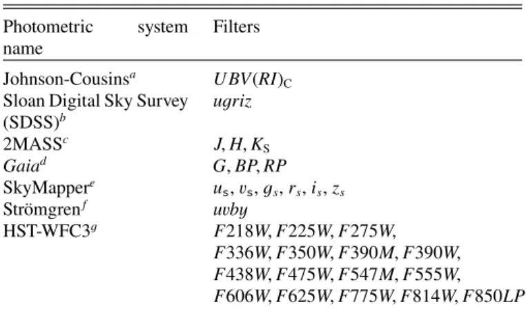
Table 1. Photometric systems used in this work and overplotted on the synthetic spectra in Fig.4.
Photometric system
name
Filters
Johnson-Cousinsa U BV(RI)
C
Sloan Digital Sky Survey (SDSS)b ugriz 2MASSc J, H, K S Gaiad G, BP, RP SkyMappere u s, vs, gs, rs, is, zs Strömgrenf uvby HST-WFC3g F218W, F225W, F275W, F336W, F350W, F390M, F390W, F438W, F475W, F547M, F555W, F606W, F625W, F775W, F814W, F850LP References.(a)Bessell & Murphy(2012),(b)Doi et al.(2010),(c)Cohen
et al.(2003),(d)Jordi et al.(2010),(e)Bessell et al.(2011),( f ) Bessell
(2011),(g)Deustua et al.(2016).
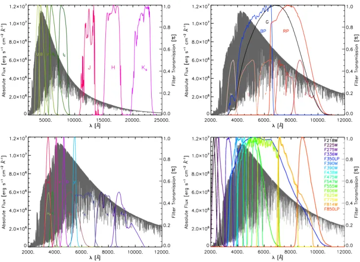
synthetic colours in the Johnson-Cousins, SDSS, 2MASS, Gaia, SkyMapper, Strömgren, HST-WFC3, and Gaia systems (Table1 and Fig.4for a comparison of the solar spectrum with the filter transmission curves studied here). For the HST-WFC3 systems our tables are provided in the VEGA, ST, and AB systems.
A full characterisation of the Gaia photometric system, including zero-points and standardisation is expected to be released in 2018. In this work, we used the transmission curves available from the ESA website4, and computed Gaia colours following Jordi et al. (2010). We fixed Vega’s magnitudes to be G = BP = RP = 0.03, and for the absolute calibration used a Kurucz synthetic Vega spectrum rescaled to the measured flux value at 5556 Å fromMegessier(1995).
Similarly to Casagrande & VandenBerg (2014), instead of colour indices we provide bolometric corrections in different bands (TableB.1 and 4–7, available at the CDS) because they are more versatile and can be rearranged in any colour combina-tion, as follows from Eqs. (3) and (4). The bolometric magnitude is defined as
MBol= −2.5 log
L L
+ MBol, , (2)
where we adopt MBol, = 4.74. It follows that the bolometric
correction in a given band BCζ is
BCζ = mBol− mζ = MBol− Mζ, (3)
where the lower and upper cases refer to apparent and absolute magnitudes, respectively. From this it follows that colour indices can be obtained from the difference in bolometric corrections, where ζ and η are two given bands:
ζ − η = mζ− mη= BCη− BCζ. (4)
Thus, in the rest of the paper when we talk about synthetic colours, these have been obtained as differences in bolometric corrections from our tables.
4 https://www.cosmos.esa.int/web/gaia/
Fig. 4.Synthetic spectrum of the solar simulation at full spectral resolution in the spectral range 2000–25 000 Å (grey, top panel) and 2000–12 000 Å (central and bottom panels). Several system response functions (Table1), from which synthetic colours have been computed, are overplotted. Johnson-Cousins system response functions (U, B, V, Rc, Ic) are plotted in green and 2MASS in pink-violet (top left panel); SDSS (u, g, r, i, z) in yellow-red and Gaia (BP, RP, G) (top right panel); Strömgren (uvby) in red-blue and SkyMapper (us, vs, gs, rs, is, zs) (bottom left panel); and the
15 filters of the HST-WFC3 (bottom right panel). For clarity, SDSS and SkyMapper functions are normalised to 0.5.
4.1. Microturbulence
The stellar surface convection produces a velocity field where the emerging spectral lines form. The Doppler broadening of these lines is a direct consequence of the velocity field in these crucial layers (Asplund et al. 2000b;Nordlund et al. 2009). In traditional 1D models, this effect can be accounted for by the use of arbitrary micro- and macroturbulence parameters. Full 3D line formation calculations using 3D RHD simulations have demonstrated that in late-type stars the required non-thermal Doppler line broadening is fully included in the convection-related motions of the stellar atmosphere (e.g. Collet et al. 2007). One-dimensional microturbulence represents the small-scale end of turbulent motions and is applied to the spectral line absorption coefficient. It affects the strong lines to a greater extent, reduc-ing their saturation, and to a lesser extent the widths of weak lines. For 1D-based SEDs, microturbulence partly redistributes the flux in spectral regions probed by the photometric systems, in particular in regions crowded with lines towards the blue and the ultraviolet, and in filters with smaller wavelength coverages (Casagrande & VandenBerg 2014).
The values of the microturbulence parameters are usually determined by comparing synthetic and observed spectral line profiles and line strengths and often using a depth-independent value. For reference, a typical value for dwarfs and subgiants is around 1−1.5 km s−1, which increases to 2−2.5 km s−1 for stars
on the red giant branch (e.g. Gray et al. 2001). A constant value of 2 km s−1 is usually assumed in large grids of synthetic stel-lar spectra (Castelli & Kurucz 2004;Brott & Hauschildt 2005). To compute our 1D hydrostatic comparison models, we explored different values of microturbulence: 0, 1, and 2 km s−1. We found that there is no clear and no unique relation between microtur-bulence and the stellar parameters, as reported by Casagrande & VandenBerg (2014). For clarity we adopted, as a guiding example, a value of 1 km s−1when performing 1D calculations.
4.2. Three-dimensional versus one-dimensional bolometric differences in correction
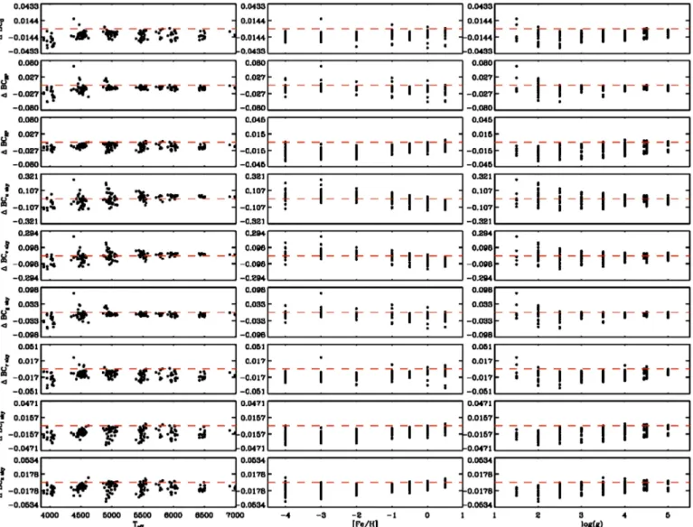
The figures in the Appendix display the bolometric corrections between 3D simulations and the corresponding 1D hydrostatic models with microturbulence = 1 km s−1. The values of BC are
reported in Table B.1 to Table 8 for all the filters and, to retrieve the absolute colours, Eqs. (3) and (4) should be used. Considering the SDSS, SkyMapper, 2MASS, and HST-WFC3 systems, the overall deviations are limited to small fraction (less than 5%) from BCr to BCKs, but they increase to 10% for
BCu and in BCg(SDSS) and for BCgsky, BCvsky, and BCusky
(SkyMapper) where the optical and line crowded region of the spectrum is probed with rather narrow filters (Fig.4, bottom); these differences decline with increasing effective temperature.
Fig. 5. Flux normalised to the continuum for the solar simulation (Table B.1) in the RVS range (8400–8900 Å). The Fe I lines (black arrows) are fromBigot & Thévenin(2006), while the Ca II triplet are indicated with red arrows.
This behaviour is more or less visible for all the photomet-ric systems; there is no clear correspondence of ∆BC with the other stellar parameters. On a broad scale, the wide infrared photometric systems like 2MASS (BCHand BCKs) and optical
Gaia(BCG) display a noticeable offset with respect to∆BC =
0.0. This is due to a redistribution of the spectral energy flux among the different filters and is a direct effect of the impact of 3D dynamics and thermodynamic structure on spectral line formation.
Gaiaphotometric systems return 3D and 1D deviations of less than 3% with higher values for the bluer system (BP). This effect may be not negligible and should become important for future releases of Gaia data. For this purpose, part of the spec-tra presented in this work have already been provided to Gaia consortium-CU85.
5. Convective velocity shifts for RVS
Measurements of stellar radial velocities are fundamental in order to determine stellar space velocities. This is needed, for example to investigate the kinematic structure of stellar popula-tions in the Galaxy or to monitor for radial velocity variapopula-tions, either of which would point to the presence of unseen com-panion(s). Convection plays a crucial role in the formation of spectral lines and deeply influences the shape, shift, and asym-metries of lines in late-type stars (e.g. Asplund et al. 2000a). These stars represent most of the objects that will be observed during the Gaia mission. Absorption lines may be blueshifted as a result of convective movements in the stellar atmosphere: bright and rising convective elements contribute more photons than the cool dark shrinking gas, and as a consequence, the absorption lines appear blueshifted (Dravins 1982). However, the convective line shift is not the same for all the spectral lines. Each line has a unique fingerprint in the spectrum that depends on line strength, depth, shift, width, and asymmetry across the granulation pattern depending on their height of formation and sensitivity to the atmospheric conditions. In this context, the line strengths play a major role (Asplund et al. 2000c).
5 For more details, see the technical note “The 3D spectral library for
BP/RP” (Chiavassa et al. 2014c).
Table 2. Central wavelength position, oscillator strength (log g f ), and excitation potential (χ) for the 20 Fe I in the spectral domain of RVS (Bigot & Thévenin 2006).
λ [Å] (log g f ) χ [eV] 8481.985 −2.097 4.1860 8514.068 −2.250 2.1980 8515.109 −2.033 3.0180 8526.667 −0.675 4.9130 8571.803 −1.134 5.0100 8582.257 −2.198 2.9900 8592.951 −0.891 4.9560 8598.829 −1.285 4.3860 8607.078 −1.419 5.0100 8611.801 −1.900 2.8450 8613.939 −1.121 4.9880 8616.280 −0.935 4.9130 8621.601 −2.369 2.9490 8674.741 −1.780 2.8310 8679.639 −1.040 4.9660 8688.623 −1.249 2.1760 8698.706 −3.464 2.9900 8699.453 −0.480 4.9550 8710.391 −0.425 4.9130 8729.147 −2.933 3.4150
The aim of the present section is to derive the overall con-vective shift for 3D simulations. First, we computed the 1D and 3D spectra with a constant resolving power of λ/∆λ = 300 000 from 8470 to 8710 Å for a limited number of 3D simulations (see Table B.1) covering stellar parameters observed by RVS (i.e. [Fe/H] ≥ −2.0). Then, from our spectra we selected only a series of non-blended Fe I lines and masked the others (Fig.5). The oscillator strengths of these Fe I lines (Table2) have been accurately determined by Bigot & Thévenin (2006) using 3D RHD simulation where the Fe I and Ca II lines are indicated. It should be noted that the synthetic spectra, when compared to the observations, have to be gravitationally redshifted (e.g. Pasquini et al. 2011) by a certain amount corresponding to the type of star considered (e.g. for the Sun it is 636.486 ± 0.024 m s−1Lindegren & Dravins 2003). Gravitational shifts for late-type dwarfs (log g ≈ 4.5) range between 0.7 and 0.8 km s−1
and they dramatically decrease with surface gravity down to 0.02–0.03 km s−1 for K giant stars with log g ≈ 1.5 (Allende
Prieto et al. 2013).
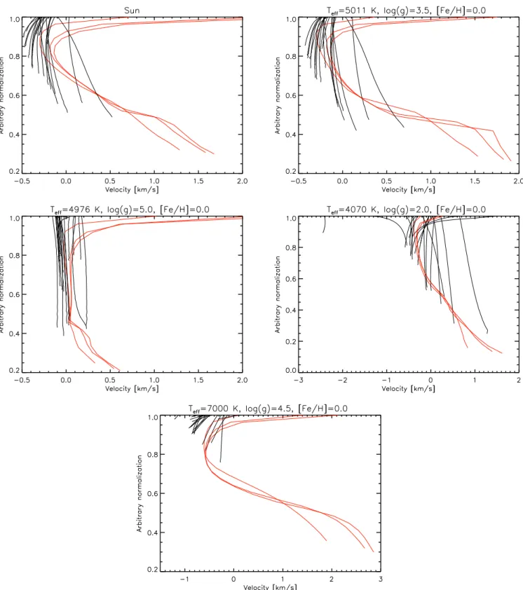
The velocity gradient through the photosphere sets the basic shape of the absorption lines in terms of asymmetry and position of the emerging intensity. One way to detect the asymmetries in the line is the bisector6. A symmetric profile has a straight
vertical bisector (i.e. in the case of hydrostatic 1D spectra). The spectral lines with C-shape bisectors are formed mostly in the upflows (granules) and therefore blueshifted. The reverse C-shapes are generally formed in downflows (Dravins et al. 1981). Reversed C-shape bisectors can be explained by a combination of a steep decline in velocities with height with a flux deficit spanning only a fraction of the red wing of the line profiles (Gray 2010). Different articles show the presence of bisectors revealing asymmetries and wavelength shifts that indicate the presence of granulation for several kinds of stars (e.g. Ramírez et al. 2008;Gray 2009).
Fig. 6.Line bisectors of the 20 Fe I lines (black) fromBigot & Thévenin(2006) and Ca II triplet (red) for five 3D simulations in the grid.
Figure6shows the line bisectors for the Fe I and Ca II triplet lines for stars with different Teff and log g, but with the same
metallicity. The gas is strongly horizontally divergent due to mass conservation and its velocities diminish with height. Weak lines (with typically high excitation potential), which form in deeper layers, are more blueshifted than strong lines whose core and part of the wings are formed in higher layers. This effect is particularly visible in Fig.6when comparing the solar bisec-tor with the hottest Teff = 7000 K simulations. In addition, the
velocity field in 3D simulations of STAGGER-grid largely affects the overall shape of the iron lines in the range of RVS and for all the stars with the strongest effects for Ca II. This has already been shown for other spectral regions (e.g. Asplund et al. 2000b; Allende Prieto et al. 2002; Ramírez et al. 2009; Pereira et al. 2013;Magic et al. 2014).
We determined the convective shift considering only Fe I and only Ca II triplet lines, we cross-correlated each 3D spectrum with the corresponding 1D by using a lag vector corresponding
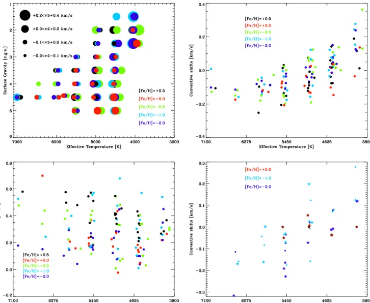
Fig. 7.Top left panel: convective shifts predicted by the 3D hydrodynamical simulations for the Gaia RVS spectral range and the Fe I lines (see text for details). Top right panel: convective shifts from Fe I lines as a function of the effective temperature of the 3D simulations in TableB.1. Bottom left panel: convective shifts from Ca II lines. Bottom right panel: comparison of convective shifts for a selected number of RHD simulations from this work (stars) with simulations with equivalent stellar parameters fromAllende Prieto et al.(2013) (circles). See Table3for details.
to radial velocities (RV) in the range −10 < v < +10 km s−1 for
Fe I, and −150 < v < +150 km s−1for Ca II triplet lines, in steps of 0.3 km s−1. These velocity ranges were chosen to largely cover
the wavelength frequency points of all the single lines. For each RV value, we Doppler-shifted the 1D spectrum and computed its cross-correlation function (CCF) with the 3D spectrum. The final step is to compute the weighted average to obtain the loca-tion of the CCF maximum, which corresponds to the actual 3D convective shifts (CS ) with respect to 1D models:
CS = R+10 −10 RV(v) · CCF (v) dv R+10 −10 CCF(v) dv (5)
Figure7displays the convective shifts for all the simulations either in the HR diagram (top left panel) or as a function of the Teff for the Fe I of Table2 (top right panel), and for the Ca II
triplet lines (bottom left panel). We found that surface gravity and metallicity have a small effect on the convective shifts, as already noticed byAllende Prieto et al.(2013). The values for the Fe I are in the range between −0.235 and +0.361 km s−1.
The convective shifts of Ca II lines are strongly redshifted (as shown by red bisectors in Fig.6) and are between −0.023 and +0.698 km s−1. In Fig.7(top right panel), there is a net
corre-lation of the convective shifts with the effective temperature: Teff / 4500 K denotes redshifts, while Teff ' 5000 K denotes
blueshifts (except for the hottest Teff≈ 7000 K). This result is in
agreement withAllende Prieto et al.(2013), who had performed the calculations for a different set of iron lines and found a milder correlation, where Teff with warmer stars tend to exhibit
larger blueshifts.
To quantify the differences in the convective shifts, we selected 26 simulations from TableB.1 with the same surface gravity, metallicity, and∆Teff < 50 K with respect to a subset of
CIFIST-grid simulations fromAllende Prieto et al.(2013). Con-vective shifts, as a function of metallicity (Table3), from RHD simulations in this work are CSStagger,[Fe/H]=0 = [−0.135, 0.142],
CSStagger,[Fe/H]=−1 = [−0.175, 0.277], and CSStagger,[Fe/H]=−2=
[−0.114, 0.119] km s−1, and from CIFIST-grid simulations CSCIFIST,[Fe/H]=0= [−0.050, 0.054], CSCIFIST,[Fe/H]=−1= [−0.170,
0.198], and CSCIFIST,[Fe/H]=−2= [−0.316, 0.119] km s−1. The
4508 4490 2.50 −1.0 0.071 0.078 −0.007 4965 4993 2.50 −1.0 −0.157 0.198 −0.355 4975 4930 3.50 −1.0 −0.007 0.021 −0.028 4956 4986 4.00 −1.0 0.123 0.026 0.097 5450 5481 3.50 −1.0 −0.175 −0.030 −0.145 5506 5473 4.50 −1.0 −0.036 −0.070 0.034 5907 5890 3.50 −1.0 −0.084 0.002 −0.086 5961 5923 4.50 −1.0 −0.043 −0.162 0.119 6435 6456 4.50 −1.0 −0.158 −0.170 0.012 4021 4001 1.50 −2.0 0.119 0.119 −0.000 4524 4500 4.00 −2.0 −0.015 −0.007 −0.008 4502 4539 4.50 −2.0 0.078 −0.011 0.089 4976 5013 4.50 −2.0 0.020 −0.072 0.092 5467 5505 3.50 −2.0 −0.075 −0.191 0.116 5480 5472 4.00 −2.0 −0.109 −0.228 0.119 5462 5479 4.50 −2.0 −0.036 −0.164 0.128 6500 6533 4.50 −2.0 −0.115 −0.316 0.201
Notes. The difference in Teffis set to be smaller than 50 K.
bottom right panel), and show smaller deviations at solar metallicity (∆CS 6 0.195 km s−1) and slightly larger
devia-tions at [Fe/H] = −1 (∆CS 6 0.370 km s−1) and [Fe/H] = −2
(∆CS6 0.221 km s−1). Apart from the possible numerical
differ-ences in the simulations and in the radiative transfer, the shift deviations may also be due to the set of spectral lines considered. The extraction of accurate radial velocities from RVS needs an appropriate wavelength calibration from convective shifts. This is directly processed in RVS pipeline using the synthetic spectra presented in this work and provided to Gaia consortium-CU67.
6. Conclusions
We provided synthetic spectra from the STAGGER-grid: – low-resolution spectra from 1000 to 200 000 Å with a
constant resolving power of λ/∆λ = 20 000;
– high-resolution spectra from 8400 to 8900 Å (Gaia RVS spectral range), with a constant resolving power of λ/∆λ = 300 000.
We used the low-resolution spectra to compute synthetic colours in the Johnson-Cousins U BV(RI)C, SDSS, 2MASS,
Gaia systems, SkyMapper, Strömgren, and HST-WFC3. We extracted the bolometric corrections for the 3D simulations and the corresponding 1D hydrostatic models. We probed that 1D
7 For more details, see the technical note “3D spectral library for RVS
radial velocities” (Chiavassa et al. 2014b) and the paper on CU6 design and performance (Sartoretti et al., in prep.).
bisectors of non-blended Fe I and Ca II triplet lines for differ-ent stars. We showed that weak lines (high excitation potdiffer-ential), which form in deeper layers, are more blueshifted than strong lines (low excitation potential), whose core and part of the wings are formed in higher layers.
As a final step to derive the overall convective shift for 3D simulations with respect to the reference 1D hydrostatic models, we cross-correlated each 3D spectrum with the corre-sponding 1D spectrum. The spanned values are between −0.235 and +0.361 km s−1. We showed a net correlation of the con-vective shifts with the effective temperature: lower Teff denotes
redshifts and higher Teff blueshifts; this result is in agreement
with Allende Prieto et al. (2013). In addition, we quantified the differences in the convective shifts between a subset of the RHD simulations in this work and the corresponding CIFIST-grid simulations. The spanned shift values from the two CIFIST-grids are similar, and show smaller deviations at solar metallicity. The extraction of accurate radial velocities from RVS spectra need an appropriate wavelength calibration from convection shifts. The spectra presented in this work have been provided to Gaia consortium-CU6 to directly process the observed spectra in RVS pipeline.
We have made all the spectra publicly available for the com-munity through the POLLUX database (Palacios et al. 2010). POLLUX8 is a stellar spectra database proposing access to
theoretical data including high-resolution synthetic spectra and spectral energy distributions from several model atmospheres. Continuous development either of the STAGGER-grid simula-tions or of the spectral synthesis calculasimula-tions will be uploaded there in the future.
Acknowledgements.L.C. gratefully acknowledges support from the Australian Research Council (grants DP150100250, FT160100402). This work was granted access to the HPC resources of Observatoire de la Côte d’Azur – Mésocentre SIGAMM.
References
Allende Prieto, C., Asplund, M., García López, R. J., & Lambert, D. L. 2002,
ApJ, 567, 544
Allende Prieto, C., Koesterke, L., Ludwig, H.-G., Freytag, B., & Caffau, E. 2013,
A&A, 550, A103
Asplund, M. 2000,A&A, 359, 755
Asplund, M., Ludwig, H., Nordlund, Å., & Stein, R. F. 2000a,A&A, 359, 669
Asplund, M., Nordlund, Å., Trampedach, R., Allende Prieto, C., & Stein, R. F. 2000b,A&A, 359, 729
Asplund, M., Nordlund, Å., Trampedach, R., & Stein, R. F. 2000c,A&A, 359, 743
Asplund, M., Grevesse, N., & Sauval, A. J. 2005, in Cosmic Abundances as Records of Stellar Evolution and Nucleosynthesis, eds. T. G. Barnes, III, & F. N. Bash,ASP Conf. Ser., 336, 25
Asplund, M., Grevesse, N., Sauval, A. J., & Scott, P. 2009,ARA&A, 47, 481
Bailer-Jones, C. A. L., Andrae, R., Arcay, B., et al. 2013,A&A, 559, A74
Bessell, M. S. 2000,PASP, 112, 961
Bessell M. S. 2011,PASP, 123, 1442
Bessell, M., & Murphy, S. 2012,PASP, 124, 140
Bessell, M., Bloxham, G., Schmidt, B., et al. 2011,PASP, 123, 789
Bigot, L., & Thévenin, F. 2006,MNRAS, 372, 609
Bigot, L., & Thévenin, F. 2008, inSF2A-2008, 3, eds. C. Charbonnel, F. Combes, & R. Samadi
Bigot, L., Mourard, D., Berio, P., et al. 2011,A&A, 534, L3
Bonifacio, P., Caffau, E., Ludwig, H.-G., et al. 2017,Mem. Soc. Astron. It., 88, 90
Brott, I., & Hauschildt, P. H. 2005, inThe Three-Dimensional Universe with Gaia, ed. C. Turon, K. S. O’Flaherty, & M. A. C. Perryman,ESA SP, 576, 565
Caffau, E., Ludwig, H.-G., Steffen, M., Freytag, B., & Bonifacio, P. 2011,
Sol. Phys., 268, 255
Cami, J., Sloan, G. C., Markwick-Kemper, A. J., et al. 2009,ApJ, 690, L122
Casagrande, L., & VandenBerg, D. A. 2014,MNRAS, 444, 392
Castelli, F., & Kurucz, R. L. 2004, ArXiv e-prints [arXiv:0405087] Chiavassa, A., Plez, B., Josselin, E., & Freytag, B. 2009,A&A, 506, 1351
Chiavassa, A., Collet, R., Casagrande, L., & Asplund, M. 2010,A&A, 524, A93
Chiavassa, A., Bigot, L., Thévenin, F., et al. 2011,J. Phys. Conf. Ser., 328, 012012
Chiavassa, A., Bigot, L., Kervella, P., et al. 2012,A&A, 540, A5
Chiavassa, A., Ligi, R., Magic, Z., et al. 2014a,A&A, 567, A115
Chiavassa, A., Thévenin, F., Magic, Z., Collet, R., & Asplund, M. 2014b,
3D spectral library for RVS radial velocities, GAIA-C8-TN-OCA-AC-001-1, Tech. Rep.
Chiavassa, A., Thévenin, F., Magic, Z., Collet, R., & Asplund, M. 2014c,The 3D spectral library for BP/RP, GAIA-C8-TN-OCA-AC-002-1, Tech. Rep.
Chiavassa, A., Pere, C., Faurobert, M., et al. 2015,A&A, 576, A13
Chiavassa, A., Caldas, A., Selsis, F., et al. 2017,A&A, 597, A94
Cohen, M., Wheaton, W. A., & Megeath, S. T. 2003,AJ, 126, 1090
Collet, R., Asplund, M., & Trampedach, R. 2007,A&A, 469, 687
Creevey, O. L., Thévenin, F., Boyajian, T. S., et al. 2012,A&A, 545, A17
Deustua, S., Baggett, S., Brammer, G., et al. 2016,WFC3 Data Handbook. Version 3.0(Baltimore: STScI) Tech. Rep.
Doi, M., Tanaka, M., Fukugita, M., et al. 2010,AJ, 139, 1628
Dravins, D. 1982,ARA&A, 20, 61
Dravins, D., Lindegren, L., & Nordlund, A. 1981,A&A, 96, 345
Gaia Collaboration (Prusti, T., et al.) 2016,A&A, 595, A1
Gray, D. F. 2009,ApJ, 697, 1032
Gray, D. F. 2010,ApJ, 721, 670
Gray, R. O., Graham, P. W., & Hoyt, S. R. 2001,AJ, 121, 2159
Gunn, J. E., Siegmund, W. A., Mannery, E. J., et al. 2006,AJ, 131, 2332
Gustafsson, B., Edvardsson, B., Eriksson, K., et al. 2008,A&A, 486, 951
Hayek, W., Asplund, M., Carlsson, M., et al. 2010,A&A, 517, A49
Hayek, W., Sing, D., Pont, F., & Asplund, M. 2012,A&A, 539, A102
Jordi, C., Gebran, M., Carrasco, J. M., et al. 2010,A&A, 523, A48
Jørgensen, U. G. 1997,IAU Symp., 178, 441
Katz, D., Munari, U., Cropper, M., et al. 2004,MNRAS, 354, 1223
Kurucz, R. L. 2005,Mem. Soc. Astron. It. Suppl., 8, 189
Lindegren, L., & Dravins, D. 2003,A&A, 401, 1185
Ludwig, H., Caffau, E., Steffen, M., et al. 2009,Mem. Soc. Astron. It., 80, 711
Magic, Z., Collet, R., Asplund, M., et al. 2013,A&A, 557, A26
Magic, Z., Collet, R., & Asplund, M. 2014, A&A, submitted [arXiv:1403.6245]
Magic, Z., Chiavassa, A., Collet, R., & Asplund, M. 2015,A&A, 573, A90
Megessier, C. 1995,A&A, 296, 771
Mihalas, D., Dappen, W., & Hummer, D. G. 1988,ApJ, 331, 815
Nordlund, A. 1982,A&A, 107, 1
Nordlund, Å., Stein, R. F., & Asplund, M. 2009,Liv. Rev. Sol. Phys., 6, 2
Palacios, A., Gebran, M., Josselin, E., et al. 2010,A&A, 516, A13
Pasquini, L., Melo, C., Chavero, C., et al. 2011,A&A, 526, A127
Pereira, T. M. D., Asplund, M., Collet, R., et al. 2013,A&A, 554, A118
Ramírez, I., Allende Prieto, C., & Lambert, D. L. 2008,A&A, 492, 841
Ramírez, I., Allende Prieto, C., Koesterke, L., Lambert, D. L., & Asplund, M. 2009,A&A, 501, 1087
Skartlien R. 2000,ApJ, 536, 465
Stempels, H. C., Piskunov, N., & Barklem, P. S. 2001, in 11th Cambridge Work-shop on Cool Stars, Stellar Systems and the Sun, eds. R. J. Garcia Lopez, R. Rebolo, & M. R. Zapaterio Osorio,ASP Conf. Ser., 223, 878
Trampedach, R., Asplund, M., Collet, R., Nordlund, Å., & Stein, R. F. 2013,ApJ, 769, 18
Fig. A.1. Bolometric correction (BC) differences computed for the photometric filters Johnson-Cousins and 2MASS with 3D simulations (TableB.1) and the corresponding 1D hydrostatic models with microturbulence = 1 km s−1:∆BC = BC
1D− BC3D. The red dashed line indicates
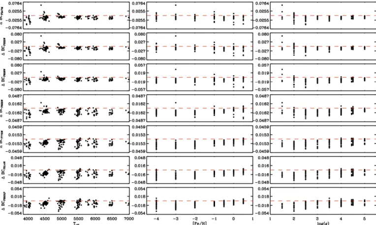
Fig. A.3.Bolometric correction differences for the HST-WFC3 provided in the VEGA system (for the ST and AB systems the differences are similar); first set of filters (Table1). The notation is the same as in Fig.A.1.
Fig. A.4.Bolometric correction differences for the HST-WFC3 provided in the VEGA system (for ST and AB systems the differences are similar); second set of filters (Table1). The notation is the same as in Fig.A.1.
Appendix B T able B. 1 . RHD simulations ’ stellar par ame ters (firs t thr ee cols.), bolome tr ic Magnitude (M bol ), and bolome tr ic cor rection (B C ) for Johnson-Cousins, 2MASS, SDSS, and Gaia sy stems (T able 1 ). Teff log g [F e/H] Mbol B CU B CB B CV B CR B CI B CJ B CH B CKs B Cu B Cg B Cr B Ci B Cz B CG B CBP B CRP 40 14.99 1.50 0.0 6.320 − 3.7 53 10 − 2.269 10 − 0.90560 − 0. 14050 0.53 170 1.588 10 2.32330 2.53 140 − 4.6 7960 − 1.63880 − 0.435 10 0.02 1 30 0.3 1 350 − 0.42 180 − 1. 17 700 0.4 40 10 40 42.38 1.50 − 1.0 6.29 1 − 3. 11 690 − 2. 1 2650 − 0.869 70 − 0. 1 3680 0.52 7 20 1.55 7 30 2.328 70 2.503 10 − 4.0 11 50 − 1.5 4990 − 0.429 70 0.02220 0.305 10 − 0.40820 − 1. 1 3330 0.43660 402 1.90 1.50 − 2.0 6.3 1 3 − 3.24590 − 2.23800 − 0.90050 − 0. 14 700 0.53 7 80 1.569 40 2.32 7 30 2.502 70 − 4. 17080 − 1.62 7 20 − 0.4 4840 0.02840 0.32220 − 0.42050 − 1. 17 860 0.4 4 480 395 1.92 1.50 − 3.0 6.389 − 3.90090 − 2.60 7 60 − 1.0 41 90 − 0. 19200 0.56 190 1.6 1 550 2.333 40 2.524 70 − 4.86820 − 1.90680 − 0.520 40 0.036 70 0.36 450 − 0.46890 − 1.33 700 0.46060 40 70.69 2.00 0.0 6.260 − 3.4 74 70 − 2. 14830 − 0.85 400 − 0. 10 740 0.5 4590 1.5 71 70 2.29980 2.49240 − 4.39 490 − 1.55290 − 0.395 70 0.0 41 40 0.3 1920 − 0.38850 − 1. 11 6 70 0.45590 4056. 19 2.00 0.5 6.2 7 6 − 3.85 400 − 2.25 7 60 − 0.92060 − 0. 148 70 0.560 10 1.60690 2.29380 2.50930 − 4.799 10 − 1.636 70 − 0.45 1 50 0.03890 0.3 43 10 − 0.4 1620 − 1. 186 40 0.45950 3899.43 2.00 − 0.5 6.4 4 7 − 3.49590 − 2.369 70 − 1.05820 − 0.25620 0.49620 1.592 10 2.40 180 2.595 40 − 4.402 70 − 1.7 8920 − 0.5 7 300 − 0.03 71 0 0.29980 − 0.5 11 30 − 1.3 1650 0.39 1 20 40 4 7.7 6 2.00 − 1.0 6.285 − 2.9 1 330 − 2.0 7 200 − 0.8 71 00 − 0. 140 40 0.52420 1.55 180 2.32650 2.49650 − 3.799 10 − 1.52820 − 0.43 160 0.0 17 40 0.30250 − 0.40 790 − 1. 1 2290 0.43260 403 7.03 2.00 − 2.0 6.296 − 2.955 40 − 2. 11 6 70 − 0.86 700 − 0. 1 33 70 0.535 70 1.55820 2.3 11 10 2.484 10 − 3.86 190 − 1.5 4 7 30 − 0.42860 0.029 10 0.3 16 40 − 0.40330 − 1. 1 31 20 0.4 4 430 40 1 3.24 2.00 − 3.0 6.322 − 3.35520 − 2.30 1 50 − 0.90580 − 0. 1 2690 0.58 160 1.58900 2.2 71 20 2.460 40 − 4.30 180 − 1.66 740 − 0.43 7 30 0.06690 0.36920 − 0.40050 − 1. 19080 0.484 70 4025.2 1 2.00 − 4.0 6.309 − 3.55980 − 2.405 40 − 0.92680 − 0. 10890 0.630 70 1.609 40 2.2 18 70 2.4 1 580 − 4.52 7 70 − 1.7 3930 − 0.43200 0. 10980 0.42 170 − 0.38300 − 1.2 1920 0.52890 3958. 11 2.50 0.0 6.382 − 3.56660 − 2.320 10 − 1.028 10 − 0.235 70 0.5 1 51 0 1.59 7 80 2.3 7 820 2.5 7 360 − 4.48420 − 1.7 43 70 − 0.5 4840 − 0.0 19 40 0.3 1 200 − 0.48920 − 1.28330 0.40 7 30 3953.50 2.50 0.5 6.38 7 − 3.80950 − 2.40 4 70 − 1. 11 480 − 0.30 4 70 0.52 7 80 1.63 4 40 2.3 7 350 2.58690 − 4.7 4 740 − 1.8 1650 − 0.6 4260 − 0.028 10 0.33840 − 0.52 750 − 1.3 71 60 0.40560 3899.65 2.50 − 0.5 6.4 4 7 − 3.38240 − 2.35 4 70 − 1.08 7 20 − 0.28 100 0.50300 1.600 10 2.40 430 2.59230 − 4.28350 − 1.80050 − 0.60 420 − 0.0 4080 0.3 1030 − 0.522 70 − 1.338 10 0.39050 4063. 17 2.50 − 1.0 6.268 − 2.7 8900 − 2.03250 − 0.868 10 − 0. 1 3650 0.53330 1.55 190 2.3 1450 2.48 1 20 − 3.66800 − 1.5 1 230 − 0.42 7 30 0.02380 0.3 10 40 − 0.40060 − 1. 11 1 50 0.43930 403 7.59 2.50 − 2.0 6.296 − 2.7 7 250 − 2.05380 − 0.85520 − 0. 1 25 40 0.53900 1.55 450 2.295 40 2.46930 − 3.66 430 − 1.5 1 240 − 0.4 17 80 0.03300 0.3 1850 − 0.39290 − 1. 10840 0.4 4 790 40 42.85 2.50 − 3.0 6.290 − 2.93 700 − 2. 11 11 0 − 0.83090 − 0.090 10 0.59520 1.5 7 280 2.2 14 40 2.40930 − 3.85 7 80 − 1.52630 − 0.39 140 0.08580 0.3 7500 − 0.35830 − 1. 10360 0.500 40 395 1.8 7 2.50 − 4.0 6.389 − 3.269 10 − 2.300 40 − 0.89860 − 0.09830 0.63 7 60 1.6 1 51 0 2. 16 480 2.38 1 20 − 4.2 1420 − 1.669 40 − 0.4 1890 0. 11 61 0 0.43080 − 0.36630 − 1. 18290 0.53650 4 4 7 2.00 1.50 − 1.0 5.852 − 2.2 1 550 − 1.56 460 − 0.5 1 380 0.0 7 860 0.629 40 1.46 7 70 2.05830 2.20 1 20 − 3.090 40 − 1.0 49 10 − 0. 17990 0. 1 5820 0.35350 − 0. 18650 − 0.7 6800 0.55020 4384.6 4 1.50 − 3.0 5.938 − 2.6 1 300 − 1.8 1900 − 0.6 1 560 0.05090 0.66850 1.5 1840 2.0 7 8 70 2.23 480 − 3.5 4550 − 1.25530 − 0.229 70 0. 18080 0.4 11 00 − 0.22330 − 0.892 70 0.5 7920 455 4.69 2.00 0.0 5.7 7 2 − 2.4 4380 − 1.5 4 790 − 0.46 7 30 0. 1 3820 0.65260 1.468 10 2.00 7 20 2. 16230 − 3.33 11 0 − 1.0 1620 − 0. 11 140 0. 189 70 0.36 460 − 0. 145 40 − 0.7 19 70 0.5 7920 4 46 1.6 7 2.00 − 0.5 5.862 − 2.292 70 − 1.5 7500 − 0.52280 0.08 1 50 0.629 70 1.4 71 80 2.06290 2.20930 − 3. 16 7 70 − 1.06080 − 0. 17 630 0. 1 58 10 0.35 420 − 0. 18 7 60 − 0.7 7 230 0.55 100 4 498.9 7 2.00 − 1.0 5.826 − 2.02690 − 1.49220 − 0.50 11 0 0.0 7 7 20 0.6 1920 1.452 10 2.0 4650 2. 184 10 − 2.89380 − 1.003 70 − 0. 17 790 0. 149 40 0.3 41 40 − 0. 18 180 − 0.7 4320 0.5 4090 4 452.9 4 2.00 − 2.0 5.8 71 − 2.06200 − 1.55860 − 0.53 160 0.06 1 50 0.62690 1.466 40 2.05 450 2. 19950 − 2.9 4 7 80 − 1.060 70 − 0.20060 0. 1 5090 0.356 70 − 0. 19 7 70 − 0.7 82 70 0.5 4 490 4 455.7 7 2.00 − 3.0 5.868 − 2. 19880 − 1.62250 − 0.5 4530 0.0 7 300 0.65900 1.48290 2.03060 2. 18220 − 3. 10880 − 1. 11 000 − 0. 19620 0. 17 840 0.39 140 − 0. 19 1 20 − 0.80530 0.5 7 330 4 485.3 7 2.00 − 4.0 5.839 − 2. 18230 − 1.6 11 50 − 0.53590 0.085 40 0.6 74 70 1.48090 2.00600 2. 1 5 740 − 3. 10 140 − 1. 10 450 − 0. 185 10 0. 19360 0.405 70 − 0. 17930 − 0.79680 0.58 790 4533.90 2.50 0.0 5.792 − 2.42220 − 1.5 43 40 − 0.48380 0. 1 2230 0.6 41 40 1.46840 2.02900 2. 17920 − 3.3 11 20 − 1.02400 − 0. 1 2 7 60 0. 17 660 0.35660 − 0. 1 5 7 70 − 0.7 30 70 0.56 7 30 4 4 70.9 7 2.50 0.5 5.853 − 2.96950 − 1.69 7 80 − 0.5 4020 0. 11 300 0.65080 1.508 70 2.05830 2.22920 − 3.893 40 − 1. 1 36 10 − 0. 143 10 0. 18090 0.3 7 280 − 0. 17980 − 0.79 450 0.5 7530 4503.3 4 2.50 − 0.5 5.822 − 2. 14 420 − 1.5 11 00 − 0.50 420 0.089 10 0.62890 1.45 71 0 2.0 4320 2. 182 70 − 3.0 1490 − 1.0 1820 − 0. 16560 0. 1 59 40 0.3 4990 − 0. 17 61 0 − 0.7 4 480 0.55090 4508.09 2.50 − 1.0 5.8 17 − 1.92660 − 1.46250 − 0.50 400 0.0 7 2 70 0.6 11 60 1.4 4500 2.0 4 480 2. 17960 − 2.7 8 7 80 − 0.99 160 − 0. 18090 0. 142 10 0.33360 − 0. 18380 − 0.7 3 71 0 0.533 70 4 426.0 4 2.50 − 2.0 5.89 7 − 1.96 700 − 1.5 4550 − 0.5 49 40 0.0 4 450 0.60950 1.46 430 2.06960 2.2 1620 − 2.84060 − 1.063 70 − 0.2 1680 0. 1 32 70 0.3 41 80 − 0.2 11 80 − 0.79080 0.52 790 4 4 7 7.40 2.50 − 3.0 5.84 7 − 1.95290 − 1.532 10 − 0.52230 0.0 7420 0.6 46 70 1.463 70 2.00 7 70 2. 160 10 − 2.84360 − 1.0 4 790 − 0. 190 10 0. 16890 0.3 7590 − 0. 18320 − 0.7 70 40 0.562 70 4535.29 2.50 − 4.0 5.79 1 − 1.84 490 − 1.4 7 630 − 0.49 41 0 0.09330 0.66230 1.45020 1.96320 2. 11 390 − 2.7 40 40 − 1.008 10 − 0. 16990 0. 18550 0.38 71 0 − 0. 16 180 − 0.7 3980 0.5 7 7 80 4508.6 7 3.00 0.0 5.8 17 − 2.43240 − 1.559 40 − 0.50960 0. 10690 0.63360 1.4 71 90 2.05230 2. 19880 − 3.32 140 − 1.05050 − 0. 14 450 0. 166 70 0.35230 − 0. 17 220 − 0.7 5060 0.55840 4 490.40 3.00 0.5 5.83 4 − 2.82400 − 1.65 450 − 0.53 4 70 0. 11 420 0.6 4960 1.49830 2.05 480 2.2 17 50 − 3.7 4320 − 1. 11 560 − 0. 14020 0. 18030 0.3 7020 − 0. 17 5 70 − 0.7 81 40 0.5 7 380 4503.05 3.00 − 1.0 5.822 − 1.89600 − 1.46 140 − 0.5 1820 0.066 70 0.60620 1.4 4 450 2.05290 2. 18560 − 2.7 5320 − 1.00280 − 0. 18660 0. 1 3630 0.329 10 − 0. 19030 − 0.7 4390 0.52820 4559.7 6 3.00 − 2.0 5.7 68 − 1.66 4 70 − 1.38800 − 0.4 7 6 70 0.08 100 0.6 1 51 0 1.422 70 1.989 70 2. 1 2 750 − 2.52520 − 0.93990 − 0. 170 70 0. 14680 0.33350 − 0. 16840 − 0.70350 0.536 70 4555.30 3.00 − 3.0 5.7 7 2 − 1.6 7 820 − 1.4 11 50 − 0.4 7 620 0.09230 0.6 4 41 0 1.43 190 1.9 49 70 2. 10060 − 2.552 10 − 0.95830 − 0. 16520 0. 17 160 0.36 490 − 0. 1 58 10 − 0.7 1090 0.56230 453 4.50 3.00 − 4.0 5.792 − 1.693 70 − 1.43200 − 0.48 7 20 0.09 140 0.65 7 60 1.438 70 1.93500 2.09 420 − 2.5 7560 − 0.98030 − 0. 17060 0. 18 1 20 0.38 190 − 0. 1 5880 − 0.7 2490 0.5 7 3 40 45 48.8 7 3.50 0.0 5.7 7 8 − 2.35 7 30 − 1.52 71 0 − 0.49890 0. 11 790 0.6 4060 1.46320 2.03 430 2. 17 580 − 3.24060 − 1.03220 − 0. 1 31 80 0. 17 550 0.35520 − 0. 16090 − 0.7 3350 0.56530 453 1.2 7 3.50 0.5 5.795 − 2.7 1 390 − 1.6 14 40 − 0.525 40 0. 1 21 80 0.65650 1.48990 2.0 4020 2. 195 70 − 3.625 70 − 1.09 490 − 0. 1 31 00 0. 18 7 60 0.3 7 3 40 − 0. 16580 − 0.7 6 460 0.5 79 40 43 4 4. 11 3.50 − 0.5 5.9 7 8 − 2.424 10 − 1.70320 − 0.6 4 420 0.02020 0.60920 1.500 70 2. 14 480 2.29230 − 3.29 750 − 1.2 1 390 − 0.24690 0. 1 2480 0.3 4900 − 0.250 70 − 0.8 7 740 0.524 10 45 7 3.06 3.50 − 1.0 5.7 55 − 1.7 84 70 − 1.39920 − 0.486 70 0.089 40 0.6 1 390 1.4269 0 2.0 1 21 0 2. 14 1 20 − 2.63660 − 0.955 40 − 0. 1 5930 0. 14840 0.32930 − 0. 16 750 − 0.70500 0.53 750 4508.84 3.50 − 2.0 5.8 16 − 1.7 2960 − 1.43 71 0 − 0.50 7 80 0.0 71 00 0.6 1480 1.43680 2.00 740 2. 1 5330 − 2.58590 − 0.98660 − 0. 183 70 0. 14390 0.33 7 70 − 0. 18240 − 0.7 3290 0.535 40 45 71 .3 4 3.50 − 3.0 5.7 5 7 − 1.59330 − 1.38 170 − 0.46 480 0. 10020 0.6 49 40 1.42240 1.9 1 350 2.0 7 260 − 2.45980 − 0.93 71 0 − 0. 1 5650 0. 17 7 70 0.36800 − 0. 14850 − 0.69500 0.56 7 60 4620.85 3.50 − 4.0 5.7 10 − 1.46630 − 1.326 10 − 0.4 45 40 0. 10 7 80 0.65 4 70 1.40 480 1.8 7 300 2.03 1 30 − 2.33620 − 0.90080 − 0. 14800 0. 18350 0.3 70 40 − 0. 1 36 10 − 0.6 71 20 0.5 7 240 4524.22 4.00 0.0 5.802 − 2.43030 − 1.5 7480 − 0.53 140 0. 10 7 60 0.6 4220 1.4 7 2 70 2.05380 2. 19560 − 3.3 11 40 − 1.083 10 − 0. 14 460 0. 17 420 0.35930 − 0. 17 4 40 − 0.7 62 70 0.56 480 45 49.22 4.00 0.5 5.7 7 8 − 2.65660 − 1.6 11 50 − 0.53 480 0. 11 9 40 0.663 40 1.48930 2.036 70 2. 18880 − 3.56000 − 1. 10 480 − 0. 1 3 4 40 0. 19200 0.3 7930 − 0. 16630 − 0.7 6890 0.583 40 4 4 41 .7 7 4.00 − 0.5 5.88 1 − 2.28050 − 1.60600 − 0.583 40 0.06360 0.62690 1.4 79 40 2.088 10 2.22950 − 3. 148 10 − 1. 1 31 50 − 0. 19600 0. 1 50 70 0.35 490 − 0.20920 − 0.8 1060 0.5 4 490 458 7. 16 4.00 − 1.0 5.7 42 − 1.79580 − 1.400 10 − 0.48 7 60 0.09840 0.620 10 1.426 70 2.003 10 2. 1 33 10 − 2.6 4530 − 0.96 180 − 0. 14950 0. 1 5580 0.33330 − 0. 16230 − 0.70200 0.5 4390 4524.9 7 4.00 − 2.0 5.80 1 − 1.7 2580 − 1.429 10 − 0.50050 0.084 70 0.62 750 1.43500 1.980 70 2. 1 31 30 − 2.5 7980 − 0.98 180 − 0. 16980 0. 1 5 7 30 0.3 48 10 − 0. 17090 − 0.7 23 10 0.5 4 790 45 17 .6 4 4.00 − 3.0 5.808 − 1.66 100 − 1.42450 − 0.48450 0.09 7 20 0.659 10 1.436 70 1.90820 2.08050 − 2.52650 − 0.9 7 230 − 0. 16350 0. 18420 0.382 10 − 0. 1 5380 − 0.7 1680 0.5 75 70 4580.60 4.00 − 4.0 5.7 48 − 1.495 10 − 1.353 10 − 0.45580 0. 10980 0.66660 1.4 1430 1.85260 2.026 10 − 2.36350 − 0.922 70 − 0. 149 40 0. 193 10 0.38520 − 0. 1 3590 − 0.68330 0.58300 4532.22 4.50 0.0 5.79 4 − 2.462 10 − 1.59380 − 0.5 4300 0. 11 020 0.652 10 1.4 7 61 0 2.0 4950 2. 19 140 − 3.33990 − 1. 10600 − 0. 14280 0. 18240 0.36800 − 0. 17 400 − 0.7 71 20 0.5 7 240 45 43. 1 5 4.50 0.5 5.7 83 − 2.65550 − 1.6 41 10 − 0.55840 0. 11 090 0.6 71 00 1.495 40 2.0 4080 2. 193 70 − 3.55 180 − 1. 140 40 − 0. 14560 0. 195 40 0.388 10 − 0. 17 420 − 0.7 89 70 0.58690 4383.32 4.50 − 0.5 5.939 − 2.4 42 10 − 1.702 70 − 0.635 40 0.0 46 70 0.633 70 1.49980 2. 11 1 50 2.259 40 − 3.3 1 230 − 1.22 1 50 − 0.2 1880 0. 1 51 00 0.36 7 80 − 0.23090 − 0.86 400 0.5 4 7 70 4569.29 4.50 − 1.0 5.7 59 − 1.88 740 − 1.4 4200 − 0.50 7 20 0. 10 140 0.63080 1.43 7 60 2.008 70 2. 14 160 − 2.7 3 700 − 1.00230 − 0. 14850 0. 16 4 70 0.3 45 10 − 0. 16530 − 0.7 2080 0.553 10 4502.45 4.50 − 2.0 5.823 − 1.80 750 − 1.46 400 − 0.5 11 40 0.09260 0.6 4530 1.4 4530 1.96500 2. 1 2500 − 2.66330 − 1.0 11 20 − 0. 16520 0. 17 31 0 0.36 750 − 0. 16 7 20 − 0.7 3560 0.56 420 4526.03 5.00 0.0 5.800 − 2.53060 − 1.63 450 − 0.56 170 0. 11 0 40 0.665 40 1.48360 2.0 4650 2. 19060 − 3.406 70 − 1. 14 4 70 − 0. 145 10 0. 19250 0.38 170 − 0. 17 6 40 − 0.7 8950 0.58260
T able B. 1 . continued. Teff log g [F e/H] Mbol B CU B CB B CV B CR B CI B CJ B CH B CKs B Cu B Cg B Cr B C 4 4 4 7. 10 5.00 − 0.5 5.8 7 6 − 2.38690 − 1.65 7 20 − 0.59 700 0.08 140 0.65580 1.48830 2.06250 2.2 1000 − 3.25500 − 1. 17990 − 0. 18080 0. 17 4535.4 7 5.00 − 1.0 5.79 1 − 2.02 1 30 − 1.50860 − 0.53300 0. 10 480 0.65280 1.45520 2.00600 2. 146 70 − 2.8 7420 − 1.06 100 − 0. 14990 0. 18 488 1.3 1 2.00 0.0 5.4 7 2 − 1.85600 − 1.25 750 − 0.3 1 260 0.22580 0.68500 1.3 7 7 60 1.8 1 390 1.95050 − 2.7 2 7 30 − 0.7 8050 − 0.00840 0.23980 49 1 5.99 2.00 − 1.0 5.4 41 − 1.4 4220 − 1. 1 33 10 − 0.30090 0. 18660 0.65 11 0 1.33 750 1.79320 1.9 1 320 − 2.30660 − 0.70 420 − 0.0 4620 0.20 4926.40 2.00 − 2.0 5.432 − 1.3 4090 − 1. 10990 − 0.30 7 20 0. 17 860 0.65220 1.33030 1.7 7580 1.896 50 − 2.220 10 − 0.70 160 − 0.056 10 0.20220 490 7.9 4 2.00 − 3.0 5.4 48 − 1.33290 − 1. 11 580 − 0.3 1880 0. 17 220 0.65590 1.33580 1.7 7 7 30 1.90090 − 2.22 1 50 − 0.7 1 5 70 − 0.065 10 0.20260 4905.26 2.00 − 4.0 5.450 − 1.3 1800 − 1. 11 680 − 0.32 140 0. 17000 0.65 7 20 1.33590 1.7 7420 1.89900 − 2.20890 − 0.7 1960 − 0.068 10 0.202 50 1 5.9 4 2.50 0.0 5.353 − 1.62 160 − 1. 1 2 750 − 0.26 400 0.240 70 0.6 7 6 40 1.33360 1.7 51 20 1.8 74 70 − 2.48800 − 0.683 10 0.0 1 380 0.23 4950.9 7 2.50 − 0.5 5.4 10 − 1.46 41 0 − 1. 1 2260 − 0.28930 0.20 1 20 0.656 40 1.33 1 50 1.7 7560 1.89620 − 2.32290 − 0.69250 − 0.02930 0.2 11 4965.89 2.50 − 1.0 5.39 7 − 1.30 1 20 − 1.0 7 8 70 − 0.29020 0. 18260 0.63 700 1.3 1 51 0 1.7 71 30 1.885 40 − 2. 1 5 7 60 − 0.66800 − 0.0 4680 0. 19220 4939.03 2.50 − 2.0 5.42 1 − 1.22650 − 1.084 70 − 0.30980 0. 16 7 70 0.636 70 1.3 1660 1.7 68 70 1.88800 − 2.09240 − 0.68 7 70 − 0.06530 0. 18 49 48.7 4 2.50 − 3.0 5.4 1 2 − 1. 18400 − 1.0 7 21 0 − 0.3 11 90 0. 16680 0.6 4250 1.3 1 290 1.7 49 10 1.8 71 40 − 2.058 10 − 0.68 7 20 − 0.06 7 70 0. 19 4953.38 2.50 − 4.0 5.408 − 1. 1 5390 − 1.06350 − 0.3 1 300 0. 16320 0.6 4060 1.30950 1.7 4280 1.86550 − 2.03030 − 0.68490 − 0.0 71 70 0. 18830 50 10.39 3.00 0.0 5.358 − 1.60350 − 1. 1 2280 − 0.26930 0.23 460 0.6 7050 1.33290 1.7 5990 1.88080 − 2.46850 − 0.68320 0.00800 0.23 4963. 1 5 3.00 0.5 5.399 − 2.0 1830 − 1.22030 − 0.28690 0.25 740 0.69550 1.3 7 290 1.7 86 10 1.92 160 − 2.90900 − 0.7 4 41 0 0.028 10 0.25630 49 1 2.9 1 3.00 − 0.5 5.4 4 4 − 1.48350 − 1. 143 70 − 0.3 10 40 0. 18 750 0.6 48 70 1.3 4060 1.808 10 1.92460 − 2.339 10 − 0.7 14 70 − 0.0 4 420 0.20 4990.00 3.00 − 1.0 5.3 7 6 − 1.23520 − 1.058 70 − 0.28900 0. 180 10 0.63000 1.30 4 40 1.7 61 30 1.8 7 240 − 2.08530 − 0.656 40 − 0.0 4 790 0. 18620 499 1.62 3.00 − 2.0 5.3 75 − 1. 10840 − 1.0 4 4 40 − 0.29980 0. 16590 0.625 10 1.29330 1.7 3 740 1.85 460 − 1.96 400 − 0.65950 − 0.06 400 0. 17 49 70.32 3.00 − 3.0 5.393 − 1.08960 − 1.05 480 − 0.3 1 250 0. 16 100 0.63320 1.29860 1.7 2860 1.85230 − 1.95230 − 0.6 7 740 − 0.0 7 250 0. 18260 5005.0 1 3.00 − 4.0 5.363 − 1.02090 − 1.02550 − 0.306 70 0. 1 5890 0.62840 1.283 70 1.70360 1.826 70 − 1.88520 − 0.660 40 − 0.0 7 3 70 0. 17 50 11 .53 3.50 0.0 5.35 7 − 1.60830 − 1. 11 830 − 0.2 71 40 0.232 10 0.66630 1.33220 1.7 66 70 1.884 40 − 2.4 71 70 − 0.68 1 50 0.00630 0.22 4988.9 1 3.50 0.5 5.3 7 7 − 1.9 45 40 − 1. 19200 − 0.28030 0.25 750 0.69200 1.36290 1.7 7 6 40 1.90 7 60 − 2.83360 − 0.7 2660 0.02990 0.25360 49 17 .82 3.50 − 0.5 5.439 − 1.4 75 40 − 1. 1 39 40 − 0.3 1 360 0. 18630 0.6 4600 1.33880 1.8 1020 1.92450 − 2.328 10 − 0.7 1460 − 0.0 4500 0. 19960 49 75.93 3.50 − 1.0 5.388 − 1.23620 − 1.06800 − 0.299 70 0. 17 4 70 0.62560 1.30 7 30 1.7 7 390 1.88400 − 2.08 140 − 0.66 750 − 0.053 40 0. 18 5036.62 3.50 − 2.0 5.336 − 1.03 4 70 − 1.0 1790 − 0.29250 0. 166 10 0.6 17 10 1.2 7520 1.7 1 280 1.82 790 − 1.882 70 − 0.6 4050 − 0.06 1 50 0. 17 50 4 7.83 3.50 − 3.0 5.326 − 0.96660 − 1.00 740 − 0.29 740 0. 162 10 0.622 10 1.26 750 1.68 170 1.802 70 − 1.82030 − 0.6 4280 − 0.06 790 0. 17 490 50 4 7.65 3.50 − 4.0 5.326 − 0.92830 − 1.003 40 − 0.30 4 40 0. 1 5 450 0.6 1880 1.26280 1.6 7 2 70 1.79580 − 1.7 8380 − 0.6 4680 − 0.0 7 650 0. 17000 4992.30 4.00 0.0 5.3 74 − 1.65 750 − 1. 1 39 70 − 0.28430 0.229 40 0.66690 1.33920 1.7 81 80 1.899 40 − 2.5 19 40 − 0.70 140 0.00290 0.22 5083.68 4.00 0.5 5.295 − 1.8 1620 − 1. 1 2350 − 0.249 70 0.2 7 320 0.69200 1.33530 1.7 31 00 1.85530 − 2.698 10 − 0.6 7430 0.050 10 0.25840 49 10.4 7 4.00 − 0.5 5.4 46 − 1.50 71 0 − 1. 1 5360 − 0.32320 0. 186 70 0.6 4 700 1.3 4290 1.8 1920 1.93320 − 2.35 7 60 − 0.7 29 40 − 0.0 4 480 0.20080 4956.7 8 4.00 − 1.0 5.405 − 1.26990 − 1.08980 − 0.3 1 280 0. 17 380 0.62680 1.3 1480 1.7 8840 1.899 40 − 2. 11 1 50 − 0.68840 − 0.05 490 0. 18240 5059.6 4 4.00 − 2.0 5.3 16 − 1.00690 − 1.0 1 250 − 0.28900 0. 16920 0.6 1650 1.26 7 60 1.69860 1.8 14 70 − 1.84930 − 0.635 70 − 0.05 750 0. 17 50 49.09 4.00 − 3.0 5.325 − 0.95 400 − 1.0 1840 − 0.29950 0. 16 420 0.62660 1.26650 1.66930 1.79600 − 1.80280 − 0.650 70 − 0.06660 0. 179 50 7 2.9 4 4.00 − 4.0 5.30 4 − 0.88 740 − 0.999 70 − 0.30200 0. 1 5690 0.6 1980 1.25250 1.6 4 71 0 1.7 7460 − 1.7 3 790 − 0.6 4 4 40 − 0.0 7400 0. 17 4982.2 7 4.50 0.0 5.383 − 1.7 2500 − 1. 16 460 − 0.29680 0.23 170 0.6 7060 1.3 46 10 1.79300 1.9 11 40 − 2.58520 − 0.7 24 70 0.00 480 0.23 5056.36 4.50 0.5 5.3 19 − 1.88 71 0 − 1. 1 5520 − 0.26 7 60 0.26980 0.69220 1.3 45 70 1.7 51 90 1.8 7 680 − 2.7 6 700 − 0.70 4 40 0.0 46 10 0.258 4953.63 4.50 − 1.0 5.408 − 1.30860 − 1. 10260 − 0.3 1920 0. 17 860 0.63060 1.3 1920 1.79 400 1.90580 − 2. 14 7 80 − 0.70 140 -0.050 10 0. 18690 49 7 6. 19 4.50 − 2.0 5.388 − 1. 1 2990 − 1.0 7590 − 0.3 1 240 0. 17020 0.630 70 1.29880 1.7 3600 1.86 1 50 − 1.9 71 10 − 0.68450 − 0.06050 0. 18430 50 79.8 1 4.50 − 3.0 5.299 − 0.93 4 40 − 1.00930 − 0.28990 0. 17 290 0.632 70 1.25 750 1.63920 1.7 7090 − 1.7 81 10 − 0.6 41 50 − 0.05 750 0. 186 4969.79 4.50 − 4.0 5.39 4 − 0.99560 − 1.06860 − 0.32560 0. 1 5 7 60 0.6 4080 1.28800 1.6 7 600 1.8 1900 − 1.84 7 80 − 0.69690 − 0.0 7950 0. 18 49 7 6.20 5.00 0.0 5.388 − 1.80 450 − 1. 18960 − 0.30900 0.23590 0.6 7520 1.35290 1.80360 1.92 170 − 2.663 40 − 0.7 4840 0.00890 0.23660 4953.82 5.00 0.5 5.408 − 2.069 40 − 1.26350 − 0.32520 0.25260 0.69 740 1.380 40 1.8 11 50 1.9 4240 − 2.9 48 10 − 0.802 70 0.023 70 0.25 4860.02 5.00 − 0.5 5.49 1 − 1.69 170 − 1.22 7 30 − 0.35980 0. 18960 0.65 750 1.36 700 1.85 490 1.9 7 290 − 2.5 4240 − 0.79 7 60 − 0.0 4 420 0.2 1030 49 71 .82 5.00 − 1.0 5.392 − 1.3 41 60 − 1. 10 480 − 0.3 16 70 0. 18980 0.63850 1.3 18 70 1.7 8420 1.89690 − 2. 179 70 − 0.70 420 − 0.03820 0. 19630 4980. 19 5.00 − 2.0 5.385 − 1. 16660 − 1.08500 − 0.30950 0. 18 140 0.6 4380 1.30 190 1.7 20 70 1.85 140 − 2.00 7 70 − 0.69000 − 0.05020 0. 19 50 43.95 5.00 − 3.0 5.329 − 0.985 40 − 1.03600 − 0.295 40 0. 17 7 80 0.6 45 40 1.2 7090 1.6 41 60 1.7 81 40 − 1.83240 − 0.660 10 − 0.055 10 0. 19 4950.0 1 5.00 − 4.0 5.4 11 − 1.02 750 − 1.086 10 − 0.32 71 0 0. 16 400 0.652 70 1.29530 1.665 40 1.8 1680 − 1.88020 − 0.70860 − 0.0 7490 0. 19850 5390.3 7 2.50 − 2.0 5.0 41 − 0.82020 − 0.79850 − 0. 19050 0.20 750 0.60 490 1. 16860 1.52300 1.624 40 − 1.69 170 − 0.46 740 − 0.005 40 0. 17 5 5 436.69 2.50 − 3.0 5.00 4 − 0.7 4360 − 0.7 6850 − 0. 19050 0. 19 7 70 0.59290 1. 14600 1.49030 1.59 1 50 − 1.6 1830 − 0.45280 − 0.0 1400 0. 163 5 459. 1 3 3.00 0.0 4.986 − 1.08 180 − 0.836 40 − 0. 1 3880 0.2 7 850 0.65050 1. 18980 1.5 1 360 1.6 17 70 − 1.9 41 70 − 0.45620 0.0 7000 0.22980 5 4 79.60 3.00 − 0.5 4.9 70 − 0.90320 − 0.79 180 − 0. 14620 0.24 700 0.62080 1. 16 170 1.49630 1.593 70 − 1.7 60 10 − 0.43380 0.03930 0. 19900 5 4 7 6.23 3.00 − 1.0 4.9 7 2 − 0.8 1420 − 0.7 81 10 − 0. 16 190 0.226 70 0.60550 1. 14950 1.489 40 1.586 70 − 1.6 71 00 − 0.43 750 0.0 18 10 0. 18220 5509. 14 3.00 − 2.0 4.9 46 − 0.698 10 − 0.7 55 40 − 0. 18090 0.20020 0.58320 1. 1 21 70 1.45 7 20 1.55500 − 1.55960 − 0.43 71 0 − 0.00860 0. 1 5 5 459.30 3.00 − 3.0 4.986 − 0.6 7 650 − 0.7 7 320 − 0.20260 0. 18300 0.5 7 740 1. 1 29 10 1.4 7530 1.5 7530 − 1.53840 − 0.460 70 − 0.02840 0. 14800 5 469.82 3.00 − 4.0 4.9 7 7 − 0.65020 − 0.7 7020 − 0.206 40 0. 17 690 0.5 71 80 1. 1 21 70 1.46520 1.56580 − 1.5 1 21 0 − 0.46 190 − 0.03 460 0. 14200 5560.38 3.50 0.0 4.906 − 0.96890 − 0.7 8500 − 0. 1 22 10 0.2 7 880 0.63 790 1. 1 5520 1.46520 1.56360 − 1.82320 − 0.4 1820 0.0 7400 0.22080 5505.98 3.50 − 0.5 4.9 49 − 0.863 10 − 0.7 8 7 30 − 0. 14 7 20 0.24 4 70 0.6 1600 1. 1 51 80 1.48590 1.58080 − 1.7 1 280 − 0.43 160 0.03 7 70 0. 19500 5 450.9 1 3.50 − 1.0 4.992 − 0.79 7 30 − 0.80 11 0 − 0. 17 530 0.2 17 80 0.60060 1. 1 5 430 1.50 7 60 1.60290 − 1.6 4 430 − 0.45 460 0.00820 0. 17 5 46 7.28 3.50 − 2.0 4.9 79 − 0.690 10 − 0.790 70 − 0. 19890 0. 190 70 0.58080 1. 1 31 70 1.480 70 1.5 7 850 − 1.5 40 10 − 0.465 40 − 0.020 10 0. 1 5330 5 4 74.46 3.50 − 3.0 4.9 74 − 0.63520 − 0.7 8550 − 0.2 11 90 0. 17 500 0.5 7030 1. 11 900 1.46290 1.563 10 − 1.48 740 − 0.4 7 21 0 − 0.03680 0. 14080 5 490.9 4 3.50 − 4.0 4.960 − 0.60 100 − 0.7 81 20 − 0.2 18 70 0. 16520 0.56060 1. 10820 1.45220 1.55 1 50 − 1.45300 − 0.4 74 10 − 0.0 46 40 0. 1 3060