Testing Stationarity with Surrogates: A Time-Frequency Approach

HAL Id: ensl-00475929

https://hal-ens-lyon.archives-ouvertes.fr/ensl-00475929

Submitted on 23 Apr 2010

HAL is a multi-disciplinary open access

archive for the deposit and dissemination of

sci-entific research documents, whether they are

pub-lished or not. The documents may come from

teaching and research institutions in France or

abroad, or from public or private research centers.

L’archive ouverte pluridisciplinaire HAL, est

destinée au dépôt et à la diffusion de documents

scientifiques de niveau recherche, publiés ou non,

émanant des établissements d’enseignement et de

recherche français ou étrangers, des laboratoires

publics ou privés.

Testing Stationarity with Surrogates: A Time-Frequency

Approach

Pierre Borgnat, Patrick Flandrin, Paul Honeine, Cédric Richard, Jun Xiao

To cite this version:

Pierre Borgnat, Patrick Flandrin, Paul Honeine, Cédric Richard, Jun Xiao. Testing Stationarity with

Surrogates: A Time-Frequency Approach. IEEE Transactions on Signal Processing, Institute of

Elec-trical and Electronics Engineers, 2010, pp.3459-3470. �10.1109/TSP.2010.2043971�. �ensl-00475929�

Testing Stationarity with Surrogates:

A Time-Frequency Approach

Pierre Borgnat, Member IEEE, Patrick Flandrin, Fellow IEEE, Paul Honeine, Member IEEE,

Cédric Richard, Senior Member IEEE, Jun Xiao

Abstract— An operational framework is developed for testing

stationarity relatively to an observation scale, in both stochastic and deterministic contexts. The proposed method is based on a comparison between global and local time-frequency features. The originality is to make use of a family of stationary surrogates for defining the null hypothesis of stationarity and to base on them two different statistical tests. The first one makes use of suitably chosen distances between local and global spectra, whereas the second one is implemented as a one-class classifier, the time-frequency features extracted from the surrogates being interpreted as a learning set for stationarity. The principle of the method and of its two variations is presented, and some results are shown on typical models of signals that can be thought of as stationary or nonstationary, depending on the observation scale used.

Index Terms— Stationarity Test, Time-Frequency Analysis,

Support Vector Machines, One-Class Classification.

I. INTRODUCTION

C

ONSIDERING stationarity is central in many signal processing applications, either because its assumption is a pre-requisite for applying most of standard algorithms devoted to steady-state regimes, or because its breakdown conveys specific information in evolutive contexts. Testing for stationarity is therefore an important issue, but addressing it raises some difficulties. The main reason is that the concept itself of “stationarity”, while uniquely defined in theory, is of-ten interpreted in different ways. Indeed, whereas the standard definition of stationarity refers only to stochastic processes and concerns the invariance of statistical properties over time, stationarity is also usually invoked for deterministic signals whose spectral properties are time-invariant. Moreover, while the underlying invariances (be they stochastic or deterministic) are supposed to hold in theory for all times, common practice allows them to be restricted to some finite time interval [3], [4], [5], possibly with abrupt changes in between [6], [7]. As an

Manuscript submitted January 30, 2009; Revised January 28, 2010. P. Borgnat, P. Flandrin and J. Xiao are with the Physics Department (UMR 5672 CNRS), Ecole Normale Supérieure de Lyon, 46 allée d’Italie, 69364 Lyon Cedex 07 France. Phone: +33(0)472728160; Fax: +33(0)4727280 80; E-mail: {Pierre.Borgnat,Patrick.Flandrin,Jun.Xiao}@ens-lyon.fr. P. Honeine is with Institut Charles Delaunay, Université de Technologie de Troyes, 12 rue Marie Curie 10010 Troyes Cedex France. Phone: +33(0)25715847 ; Fax: +33(0)25715699 ; E-mail: [email protected]. C. Richard is with Institut Charles Delaunay, Université de Technologie de Troyes and Laboratoire FIZEAU (UMR CNRS 6525), Observatoire de la Côte d’Azur, Université de Nice Sophia-Antipolis Parc Valrose, 06108 Nice Cedex 02 France Phone: +33 (0)4 92 07 63 94; Fax: +33 (0)4 92 07 63 21; E-mail: [email protected]. This work was supported in part by the ENS-ECNU Doctoral Program and ANR-07-BLAN-0191-01 StaRAC. Part of this paper was first presented at the 15th European Signal Proc. Conf. EUSIPCO-07 (Poznan, PL) [1] and at the IEEE Stat. Sig. Proc. Workshop SSP-07 (Madison, WI) [2].

example, we can think of speech that is routinely “segmented into stationary frames”, the “stationarity” of voiced segments relying in fact on periodicity structures within restricted time intervals. Those remarks call for a better framework aimed at dealing with “stationarity” in an operational sense, i.e., with a definition that would both encompass stochastic and deterministic variants, and include the possibility of its test relatively to a given observation scale.

Several attempts in this direction can be found in the literature, mostly based on concepts such as local stationarity [5]. Most of them however share the common philosophy of comparing statistics of adjacent segments, with the objective of detecting changes in the data [6], [7] and/or segmenting it over homogeneous domains [3] rather than addressing the afore-mentioned issue. Other attempts have nevertheless been made in this direction too by contrasting local properties with global ones [4], [8], but not necessarily properly phrased in terms of hypothesis testing. Among more recent approaches, we can mention those reported in [9], [10] which share some ideas with this work, but with the notable difference that they are basically model-based (whereas ours is not). Early works [11], [12] proposed a global test of stationarity based on approximate statistics of evolutionary spectra [13], which is performed as a two-step analysis of variance. The assumption of independence of time-frequency bins that are used is necessary. It is obviously and openly understood to be wrong, and may lead to stationary decision errors due to biased estimations. It is therefore the purpose of this contribution to propose and describe a different approach, using a resampling method called surrogate data, to obtain robust statistics under the hypothesis of stationarity given one observation only. It is aimed at deciding whether an observed signal can be considered as stationary, relatively to a given observation scale, and, if not, to give an index as well as a typical scale of nonstationarity.

In a nutshell, the purpose of this paper is to recast the question of stationarity testing within an operational frame-work elaborating on three main ideas: (i) stationarity as an operational property relying on one observation has to be understood in a relative sense including some observation scale as part of its definition; (ii) both stochastic and deterministic situations should be embraced by the approach so as to meet common practice; (iii) significance should be given to any test in order to provide users with some statistical characterization of the null hypothesis of operational stationarity.

The paper is organized as follows. In Sect. II, the general framework of the proposed approach is outlined, detailing the

time-frequency rationale of the method and motivating the use of surrogate data for characterizing the null hypothesis of stationarity and constructing stationary tests. A first test, from which both an index and a scale of nonstationarity can be derived, is proposed in Sect. III on the basis of spectral distance measures and of a parametric modeling of surrogates distributions. A second, non-parametric, test is introduced in Sect. IVby considering surrogates as a learning set and using a one-class classifier. In both cases, implementation issues are discussed, together with some examples supporting the efficiency of the methods. Finally, some of the many possible variations and extensions are briefly outlined in Sect. V.

II. FRAMEWORK

Second order stationary processes are a special case of the more general class of (nonstationary) harmonizable processes, for which time-varying spectra can be properly defined [14]. When the analyzed process happens to be stationary, those time-varying spectra may reduce to the classical (station-ary, time-independent) Power Spectrum Density (PSD) when suitably chosen (this holds true, e.g., for the Wigner-Ville Spectrum (WVS) [14]). In the case of more general definitions that can be considered as estimators of the WVS (e.g., spec-trograms), the key point is that stationarity still implies time-independence, the time-varying spectra identifying, at each time instant, to some frequency smoothed version of the PSD. The basic idea underlying the approach proposed here is there-fore that, when considered over a given duration, a process will be referred to as stationary relatively to this observation scale if its time-varying spectrum undergoes no evolution. In other words, stationarity in this acceptance happens if the local spectra at all different time instants are statistically similar to the global spectrum obtained by marginalization. This idea has already been pushed forward [4], but the novelty is to address the significance of the difference “local vs. global” by elaborating from the data itself a stationarized reference serving as the null hypothesis for the test (see Sect. II-C). A. A time-frequency approach

As far as only second order evolutions are to be tested, quadratic time-frequency (TF) distributions and spectra are natural tools [14]. Well-established theories exist for justifying the choice of a given TF representation. In the case of station-ary processes, the WVS is not only constant as a function of time but also equal to the PSD at each time instant. From a practical point of view, the WVS is a quantity that has however to be estimated. In this study, we choose to make use of multitaper spectrograms [15] defined as

Sx,K(t, f) = 1 K K ! k=1 S(hk) x (t, f), (1) where the {S(hk)

x (t, f), k = 1, . . . , K} stand for the K

spectrograms computed with the K first Hermite functions as short-time windows hk(t): S(hk) x (t, f) = " " " " # x(s) hk(s − t) e−i2πfsds " " " " 2 . (2)

The reason for this choice is that spectrograms can be both interpreted as estimates of the WVS for stochastic processes and as reduced interference distributions for deterministic signals [14].

In (2), the Hermite functions hk(t) are defined by

hk(t) =$(t − D)kg%(t)/

&

π1/22k_k!,

with g(t) = exp_{−t2_/2

}. In practice, such functions can be computed recursively, according to

hk(t) = g(t) Hk(t)/

&

π1/22k_k!,

where the_{Hk(t), t ∈ IN} stand for the Hermite polynomials

that obey the recursion

Hk(t) = 2tHk−1(t) − 2(k − 2)Hk−2(t), k ≥ 2

with the initialization H0(t) = 1 and H1(t) = 2 t. Being

orthonormal and maximally concentrated in TF domains with elliptic symmetry, they are a preferred family of windows for the multitaper approach which is adopted here in order to reduce estimation variance without some extra time-averaging which would be unappropriate in a nonstationary context. In practice, the multitaper spectrogram is evaluated only at N time positions_{tn, n = 1, . . . , N}, with a spacing tn+1− tn

which is an adjustable fraction—typically, one half—of the temporal width Th of the K windows hk(t).

B. Relative stationarity

The TF interpretation suggesting that suitable representa-tions should undergo no evolution in stationary situarepresenta-tions, stationarity tests can be envisioned on the basis of some comparison between local and global features. Relaxing the assumption that stationarity would be some absolute property, the basic idea underlying the approach proposed here is that, when considered over a given duration, a process will be re-ferred to as stationary relatively to this observation scale if its time-varying spectrum undergoes no evolution. Quantitatively, this corresponds to the fact that the local spectra Sx,K(tn, f ) at

all different time instants are statistically similar to the global (average) spectrum $Sx,K(tn, f )%n:= 1 N N ! n=1 Sx,K(tn, f ) (3)

obtained by marginalization. In practice, fluctuations in local spectra will always exist, be the signal stationary or not. The whole point of the paper is therefore to develop a comprehensive and operational methodology able to assess the significance of observed fluctuations.

C. Surrogates

Revisiting stationarity within the TF perspective has already been pushed forward [4], but the novelty is to address the significance of the difference “local vs. global” by elaborating from the data itself a stationarized reference serving as the null hypothesis for the test. Indeed, distinguishing between stationarity and nonstationarity would be made easier if, besides the analyzed signal itself, we had at our disposal some

reference having the same marginal spectrum while being stationary. Since such a reference is generally not available, one possibility is to create it from the data. This is the rationale behind the idea of “surrogate data”, a technique which has been introduced and widely used in the physics literature, mostly for testing linearity [16] (up to some proposal reported in [17], it seems to have never been used for testing stationarity).

For an identical marginal spectrum over the same ob-servation interval, nonstationary processes are expected to differ from stationary ones by some structured organization in time, hence in their time-frequency representation. A set of J “surrogates” is thus computed from a given observed signal, so that each of them has the same PSD as the original signal while being “stationarized”. In practice, this is achieved by destroying the organized phase structure controlling the nonstationarity, if any. To this end, the signal is first Fourier transformed, and the magnitude of the spectrum is then kept unchanged while its phase is replaced by a random sequence, uniformly distributed over [_{−π, π]. This modified spectrum is} then inverse Fourier transformed, leading to as many stationary surrogate signals as phase randomizations are operated.

To be more precise, let us assume that the observed signal is known in discrete-time (x[n], n = 1, . . . , N ) and has a discrete Fourier transform X[k] such that

x[n] = 1 N

!

k

X[k]ei2πnk/N.

Expressing X[k] in terms of its magnitude A[k] and phase Φ[k] such that X[k] = A[k]eiΦ[k]_{, a surrogate s[n] is}

con-structed from X[k] by replacing Φ[k] with an i.i.d. phase sequence Ψ[k] drawn from a uniform distribution over [_{−π, π]:}

s[n] = 1 N

!

k

A[k]eiΨ[k]_ei2πnk/N_,

from which it follows that s[n]s∗[m] = 1 N2 ! k ! l A[k]A[l]ei(Ψ[k]−Ψ[l]+2π(nk−ml)/N), Making explicit the contributions in the above double sum as: ! k ! l G[k, l] =! k  G[k, k] +! l#=k G[k, l]   and evaluating expectations regarding random quantities, we end up for the first term with:

1 N2

!

k

E{A2_[k]}ei2π(n−m)k/N ₍₄₎

and, for the second one, with 1 N2 ! k ! l#=k

E{A[k]A[l]}ei2π(nk−ml)/N_E{ei(Ψ[k]−Ψ[l])_}.

Given that the Ψ[k]’s are i.i.d. and uniformly distributed over [_{−π, π], their difference has the triangular distribution:}

Λ(ψ) = 1 4π2(1 − |ψ|/2π) time signal original time 1 surrogate time frequency marg. time frequency time frequency

average over 40 surrogates

time

marg.

time time

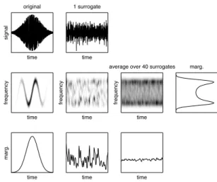
Fig. 1. Surrogates. This figure compares the TF structure of a nonstationary FM signal (1st column), of one of its surrogates (2nd column) and of an ensemble average over J = 40 surrogates (3rd column). The spectrogram is represented in each case on the 2nd line, with the corresponding marginal in time on the 3rd line. The marginal in frequency, which is the same for the three spectrograms, is displayed on the far right of the 2nd line.

over [−2π, 2π] and, therefore: E{ei(Ψ[k]−Ψ[l])_{} =}# 2π

−2π

eiψΛ(ψ)dψ = 0.

It follows that the covariance function of the surrogate s[n] reduces to (4) and, as a function of n_{− m only, it is therefore} stationary. In the practical case where A[k] is taken as the magnitude of the Fourier transform of the observed signal (i.e., of one specific realization of the process x[n]) and kept strictly unchanged for all phase randomizations, the stationary covariance of the surrogates identifies furthermore with the Fourier transform of the (global) empirical spectrum of this observation.

The effect of the surrogate procedure is illustrated in Fig.1, displaying both signal and surrogate spectrograms, together with their marginals in time and frequency. It clearly appears from this figure that, while the original signal undergoes a structured evolution in time, the recourse to phase randomiza-tion in the Fourier domain ends up with starandomiza-tionarized (i.e., time unstructured) surrogate data with identical spectrum. As compared to more standard uses of surrogate data, we underline that we are primarily interested here in second order properties in a transformed domain. In this respect, the fact that phase randomization not only destroys nonstationarity features (as expected) but also other properties in the signal by a well-known Gaussianization effect, does not play the same dramatic role as, e.g, in testing nonlinearity in some reconstructed phase-space.

III. ADISTANCE-BASED TEST

Once a collection of stationarized surrogate data has been synthesized, different possibilities are offered. The first one is to extract from them some features such as distances between local and global spectra, and to characterize the null hypothesis

of stationarity by the statistical distribution of their variation in time. This first approach is the purpose of this Section. A. Principle

Given an observed signal x(t) and its (multitaper) spectro-gram Sx,K(tn, f ), it is proposed to compare local and global

frequency features according to

{c(x)n := D (Sx,K(tn, .),$Sx,K(tn, .)%n) , n = 1, . . . , N},

(5) where D(., .) stands for some dissimilarity measure (or “dis-tance”) in frequency.

If we now label {sj(t), j = 1, . . . , J} the J surrogate

signals obtained as described previously and analyze them the same way, we end up with a new collection of distances which are a function of both time indices and randomizations, namely: {c(sj) n := D $ Ssj,K(tn, .),$Ssj,K(tn, .)%n % , n = 1, . . . , N_} (6) with j = 1, . . . , J.

As far as the intrinsic variability of surrogate data is con-cerned, the dispersion of distances under the null hypothesis of stationarity can be measured by the distribution of the J empirical variances

+

Θ0(j) = var(c(snj))n=1,...,N, j = 1, . . . , J

,

. (7) This distribution allows for the determination of a threshold γ above which the null hypothesis is rejected. The effective test is therefore based on the statistics

Θ1= var(c(x)n )n=1,...,N (8)

and takes on the form of the one-sided test: d(x) =

- _{1 if Θ}

1> γ : “nonstationarity";

0 if Θ1< γ : “stationarity”. (9)

The choice of the threshold γ will be discussed in Sect. III-E

from the distribution of Θ0 obtained with a collection of

surrogates.

Assuming that the null hypothesis of stationarity is rejected, an index of nonstationarity can furthermore be introduced as a function of the ratio between the test statistics (8) and the mean value (or the median) of its stationarized counterparts (7): INS := . Θ1 $Θ0(j)%j . (10)

If the signal happens to be stationary, INS is expected to take a value close to unity whereas, the more nonstationary the signal, the larger the index.

Finally, it has to be remarked that, whereas the tested stationarity is globally relative to the time interval T over which the signal is chosen to be observed, the analysis still depends on the window length Th of the spectrogram. Given

T , the index INS will therefore be a function of Th and,

repeating the test with different window lengths, we can end up with a typical scale of nonstationarity SNS defined as:

SNS := 1

T arg maxTh {INS(T

h)} , (11)

with Th in the range of window lengths such that the

pre-scribed threshold is exceeded in (9).

The principle of the test having been outlined, its actual implementation depends on a number of choices that have to be made and justified, regarding distances, surrogates, thresholds, etc. Many options are however offered, that are moreover intertwined. A complete investigation of all possi-bilities and their combinations will not be envisioned here but, nevertheless, key features that are important for the test to be used in practice will be highlighted in the following.

B. Test signals

Setting specific parameters in the implementation is likely to end up with performance depending on the type of nonstation-arity of the signal under test. Whereas no general framework can be given for encompassing all possible situations, two main classes of nonstationarities can be distinguished, which both give rise to a clear picture in the time-frequency plane: amplitude modulation (AM) and frequency modulation (FM). We will base the following discussions on such classes. In the first case (AM), a basic, stochastic representative of the class can be modelled as:

x(t) = (1 + m sin 2πt/T0) e(t), t ∈ T, (12)

with m ≤ 1 and where e(t) is white Gaussian noise, T0 is

the period of the AM and T the observation duration. In the second case (FM), a deterministic model can be defined as:

x(t) = sin 2π(f0t + m sin 2πt/T0), t ∈ T, (13)

with m ≤ 1 and where f0 is the central frequency of the

FM, T0its period and T the observation duration. To this FM

model, a white Gaussian noise can be added if one wants to obtain different realizations of the signal.

C. Distances

Within the chosen time-frequency perspective, the proposed test (9) amounts to compare local spectra with their average over time thanks to some “distance” (5), and to decide that stationarity is to be rejected if the fluctuation of such descrip-tors (as given by (8)) is significantly larger than what would be obtained in a stationary case with a similar global spectrum. The choice of a distance (or dissimilarity) measure is therefore instrumental for contrasting local vs. global features.

Many approaches are available in the literature [18] that, without entering into too much details, can be broadly clas-sified in two groups. In the first one, the underlying inter-pretation is that of a probability density function, one of the most efficient candidate being the well-known Kullback-Leibler (KL) divergence defined as

DKL(G, H) :=

#

Ω

(G(f) − H(f)) logG(f )

H(f )df, (14) where, by assumption, the two distributions G(.) and H(.) to be compared are positive and normalized to unity over the domain Ω. In our context, such a measure can be envisioned for (always positive) spectrograms thanks to the probabilistic

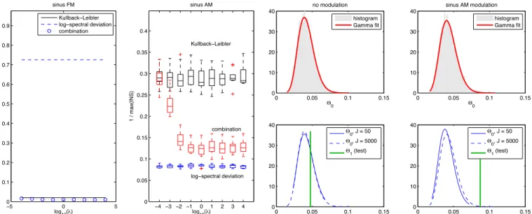
−5 0 5 0 0.1 0.2 0.3 0.4 0.5 0.6 0.7 0.8 0.9 log₁₀(!) 1 / max(INS) sinus FM −4 −3 −2 −1 0 1 2 3 4 0 0.05 0.1 0.15 0.2 0.25 0.3 0.35 0.4 1 / max(INS) log₁₀(!) sinus AM log−spectral deviation combination Kullback−Leibler Kullback−Leibler log−spectral deviation combination

Fig. 2. Choosing a distance. The inverse of the maximum value (over Th)

of the index of nonstationarity INS defined in (10) is used as a performance measure. Comparing the Kullback-Leibler (KL) divergence with the log-spectral deviation (LSD), a better result (i.e., a lower value) is obtained with KL (full line) in the FM case (left, with m = 0.03), and with LSD (dashed line) in the AM case (right, with m = 0.5). A better balanced performance is obtained when using the combined distance (dots) defined in (16): in the FM case, this measure performs best, and in the AM case it achieves a good contrast when λ ≥ 1. In the AM case, the boxplots resulting from 10 realizations of the process are displayed.

interpretation that can be attached to distributions of time and frequency [14].

A second group of approaches, which is more of a spectral nature, is aimed at comparing distributions in both shape and level. One of the simplest examples in this respect is the log-spectral deviation (LSD) defined as

DLSD(G, H) := # Ω " " " " log_{H(f )}G(f ) " " " " df. (15) Intuitively, the KL measure (14) should perform poorer than the LSD (15) in the AM case (12), because of normalization. It should however behave better in the FM case (13), because of its recognized ability at discriminating distribution shapes. In order to take advantage of both measures, it is therefore proposed to combine them in some ad hoc way as

D(G, H) := DKL( ˜G, ˜H). (1 + λ DLSD(G, H)) , (16)

with ˜G and ˜H the normalized versions of G and H, and where λ is a trade-off parameter to be adjusted. In practice, the choice λ = 1 ends up with a good performance, as justified in Fig. 2

(the performance measure used in this figure is the inverse of the maximum value (over Th) of the index of nonstationarity

INS defined in (10), i.e., an inverse measure of contrast). D. Distribution of Surrogates

The basic ingredient (and originality) of the approach is the use of surrogate data for creating signals whose spectrum is identical to that of the original one while being stationarized by getting rid of a well-defined structuration in time. Since those surrogates can be viewed as distinct, independent realizations

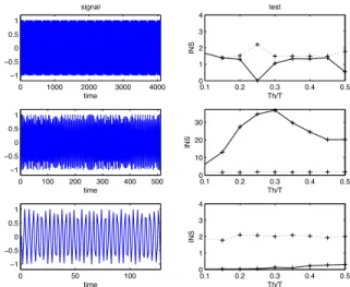
0 0.05 0.1 0.15 0 10 20 30 40 "0 no modulation histogram Gamma fit 0 0.05 0.1 0.15 0 10 20 30 40 "0 sinus AM modulation histogram Gamma fit 0 0.05 0.1 0.15 0 10 20 30 40 "₀, J = 50 "₀, J = 5000 "₁ (test) 0 0.05 0.1 0.15 0 10 20 30 40 "₀, J = 50 "₀, J = 5000 "₁ (test)

Fig. 3. Distribution based on surrogates. The top row superimposes empirical histograms of the variances (7) based on J = 5000 surrogates (grey) and their Gamma fits (full line), in the case of a white Gaussian noise without (left) and with (right) a sinusoidal AM (with m = 0.5). The bottom row compares the corresponding probability density functions, as parameterized by using J = 50 (full line) and 5000 (dashed line) surrogates. The values of the test statistics (8) computed on the analyzed signal are pictured in both cases as the vertical lines.

of the stationary counterpart of the analyzed signal, the central part of the test is based on the statistical distribution of the J variances given in (7).

When using the combined distance suggested above in Sect.

III-C, an empirical study (on both AM and FM signals) has

shown that such a distribution can be fairly well approximated by a Gamma distribution. This makes sense since, according to (7), the test statistics basically sums up squared, possibly dependent quantities which themselves result from a strong mixing likely to act as a Gaussianizer. An illustration of the relevance of this modeling is given in Fig. 3, where Gamma fits are superimposed to actual histograms in the asymptotic regime (J = 5000 surrogates). Assuming the Gamma model to hold, it is possible to estimate its 2 parameters directly from the J surrogates, e.g., in a maximum likelihood sense. In this respect, Fig. 3 also supports the claim that the “theoretical" probability density function (more precisely, its estimate in the asymptotic regime) can be reasonably well approached with a reduced number of surrogates (typically, J ≈ 50). Finally, the value of the test (8), computed on the actual signals under study, is also plotted and shown to stand in the middle of the distribution in the stationary case while clearly appearing as an outlier in the considered nonstationary situation.

As a general remark, let us emphasize that modeling the distribution is important in two (related) respects. First, based on the results of Fig. 3, this allows for using much less surrogates than a crude histogram. Second, given the estimated parameters of the model, it becomes much easier to precisely define the chosen threshold for the test (see Section III.E). One could have think of other models for the distribution, such as, e.g., the simpler situation of a χ2_{. Experimental attempts in}

0 1000 2000 3000 4000 −5 0 5 time signal 0.1 0.2 0.3 0.4 0.5 0 2 4 T_h/T INS test 0 500 1000 −4 −2 0 2 4 time 0.1 0.2 0.3 0.4 0.5 0 2 4 T_h/T INS 0 50 100 −4 −2 0 2 time 0.1 0.2 0.3 0.4 0.5 0 2 4 T_h/T INS

Fig. 4. AM example (m = 0.5). In the case of the same signal (12) observed over different time intervals (left column), the indices of nonstationarity INS (right column, full line) are consistent with the physical interpretation accord-ing to which the observation can be considered as stationary at macroscale (top row), nonstationary at mesoscale (middle row) and stationary again at microscale (bottom row). The threshold (dotted line) of the stationarity test (9) is calculated with a confidence level of 95% and represented in term of INS aspγ/"Θ0(j)#j), with J = 50. In the nonstationary case, the position of the

maximum of INS also gives an indication of a typical scale of nonstationarity.

choice of a Gamma model was therefore guided by the fact that, with two degrees of freedom, it is obviously more flexible than a χ2_{, while keeping the idea of resulting from summations}

of squared Gaussian-like quantities.

E. Threshold and Reproduction of the Null Hypothesis Given the Gamma model for the distribution of Θ0 based

on surrogates, it becomes straightforward to derive a threshold above which the null hypothesis of stationarity is rejected with a given statistical significance. The effectiveness of the procedure at reproducing the null hypothesis of stationarity has been considered elsewhere [19], and it will not be reproduced here. Based on Monte-Carlo simulations with stationary AR processes, the main finding of the results reported in [19] is that an actual number of false positives of about 6.5 % is observed for a prescribed false alarm rate of 5 %. The test appears therefore as slightly pessimistic, yet in a reasonable agreement with what expected.

F. Illustration

In order to illustrate the proposed approach and to support its effectiveness, a simple example is given in Fig. 4. The analyzed signal consists of one realization of an AM process of the form (12). Depending on the relative values of T0and

T , three regimes can be intuitively distinguished:

1) if T _{( T}0 (macroscale of observation), many

oscilla-tions are present in the observation, creating a sustained, well-established quasi-periodicity that corresponds to a form of operational stationarity;

2) if T ≈ T0 (mesoscale), emphasis is put on the local

evolutions due to the AM, suggesting to rather consider the signal as nonstationary, with some typical scale;

0 1000 2000 3000 4000 −1 −0.5 0 0.5 1 time signal 0.1 0.2 0.3 0.4 0.5 0 1 2 3 4 Th/T INS test 0 100 200 300 400 500 −1 −0.5 0 0.5 1 time 0.1 0.2 0.3 0.4 0.5 0 10 20 30 Th/T INS 0 50 100 −1 −0.5 0 0.5 1 time 0.1 0.2 0.3 0.4 0.5 0 1 2 3 4 Th/T INS

Fig. 5. FM example (m = 0.02, f0 = 0.25). The same signal (13)

is observed over different time intervals (left column). As in Fig.4 the indices of nonstationarity INS (right column, full line) leads to physical interpretation according to which the observation can be considered as stationary at macroscale (top row), nonstationary at mesoscale (middle row) and stationary again at microscale (bottom row). The threshold (dotted line) of the stationarity test (9) is calculated with a confidence level of 95% and represented in term of INS aspγ/"Θ0(j)#j), with J = 50. In the

nonstationary case, the position of the maximum of INS also gives an indication of a typical scale of nonstationarity.

3) if T _{) T}0 (microscale), no significant difference in

amplitude is perceived, turning back to stationarity. What is shown in Fig. 4 is that such interpretations of operational and relative stationarity are precisely evidenced by the proposed test. One difference between theoretical (second-order) stationarity of random processes and operational sta-tionarity that we study, and that aims at being consistent with the physical and time-frequency interpretation of what stationarity means, is that both situations where there is no change in time of second-order statistics (here at microscale), and situations where there is a regular repetition if the same feature (here at macroscale of observation) are considered as being stationary in its operational acceptance. They are moreover quantified in the sense that, when the null hypothesis of stationarity is rejected (middle diagram), both an index and a scale of nonstationarity can be defined according to (10) and (11). In the present case, the maximum value of INS is obtained for SNS = Th/T ≈ 0.2, in qualitative accordance

with the 4 AM periods entering the observation window. At this point, it is worth stressing the fact that allowing the window length to vary is an extra degree of freedom that is part of the methodology, since it permits to give sense to a notion of stationarity relatively to an observation scale. There is therefore no prior “proper” window length for a given signal, but varying it allows for the determination of a scale of stationarity (if any).

In this specific example, the data could have been referred to as cyclostationary and analyzed by tools dedicated to such processes [20]. However, it has to be stressed that no such a priori modeling is assumed in the proposed methodology, and that the existence of a typical scale of stationarity (related to the periodic correlation) naturally emerges from the analysis.

A second example, given in Fig.5, reports the same analysis done on a realization of the FM signal of the form (13). The same dependence on the relative values of T0 and T is

evident and the same three possible behaviors (observation at macroscale, mesoscale or microscale of the signal) are obtained. Also, let us further comment about a specificity of operational stationarity as tested here. For the microscale T _{) T}0, the model turns out to be almost a pure sine function

(with some added noise). The time-frequency spectrum of this signal being constant (a spectral line at frequency f0), this

signal is considered as stationary from an operational point of view, and relatively to an observation scale T that is much larger than the period of this sine 1/f0 and much lower than

period of the frequency modulation T0. Finally, let us remark

that the INS in this last case is very small as compared to the threshold: this is due to the very small variability of a sine as compared to its surrogates. This feature will be further commented when turning to the non-parametric test of the next Section.

G. Comparison to other approaches

Using surrogate data to provide users with some statistical characterization of the null hypothesis of stationarity raises the question of simply testing if the phase of the Fourier transform of x(t) is an i.i.d. sequence, as is the case with surrogates. This can be performed with classical i.i.d. Portmanteau tests such as Ljung and Box, and McLeod and Li (see, e.g, in [21]). The basic property on which these tests are based is that, for large N , the sample autocorrelation of an i.i.d. N -length sequence is i.i.d. with Gaussian distribution _{N (0, 1/N). Experiments} have been conducted using a Ljung and Box statistical test with significance level of 5%, and applied to 1000 realizations of the AM and FM test signals described in Sect. III-B. The hypothesis of i.i.d. phase sequence was accepted/rejected as reported in Table I, with respective acceptance/rejection rates that were observed over the 1000 realizations. Except in the FM case where the period is equal to the observation duration, the i.i.d. hypothesis is always accepted. It clearly appears that little information is revealed by this kind of tests, which does not involve global vs. local time-frequency features, compared with the proposed framework based on second-order time-varying spectra. Nevertheless, we can mention some interesting on-going work [22] based on a Portmanteau type test for stationarity: comparing it to the present work is beyond the scope of this paper but this would certainly deserve consideration in further studies.

Existing works on statistics of evolutionary spectra [13] raise the question of constructing test statistics to compare time-frequency characteristics of the signal under study with what is expected under the null hypothesis. This kind of strategy has been adopted in many situations, e.g., to detect time-frequency features of interest [23]. In [11], [12], the authors proposed a global test of stationarity from approximate statistics. It consists of a two-step analysis of variance induced by the chi-squared distribution. As most of works in the area, the assumption of independence of time-frequency bins that are used is necessary to derive closed-form tests. This leads

Period AM FM

T0= T /20 accepted (94%) accepted (94%)

T0= T accepted (92%) rejected (54%)

T0= 20T accepted (94%) accepted (90%)

TABLE I

RESULT OF APORTMANTEAU TEST ON THE PHASE OF THEFOURIER TRANSFORM OFx(t),FOR THEAMANDFMPROCESSES OFSECT.III-B.

THE PARAMETERS AREN = T = 1600, SNR = 10DB, m = 0.5 (AM)

AND0.02 (FM). THE RESULTS REPORTED ARE THE AVERAGE OF1000

REALIZATIONS.

to poorly informative statistics and, in the present case, to stationary decision errors. Our resampling method does not rely on this hypothesis, but considers the spectrograms of surrogate data globally to provide more informative tests.

IV. ANON-SUPERVISED CLASSIFICATION APPROACH

Besides the distance-based approach described above, we can adopt an alternative viewpoint rooted in statistical learning theory by considering the collection of surrogates as a learning set and using it to estimate the support of the distribution of stationarized data. Let us make this approach more precise. A. An overview on one-class classification

In the context considered here, the classification task is fundamentally a one-class classification problem and differs from conventional two-class pattern recognition problems in the way how the classifier is trained. The latter uses only target data to perform outlier detection. This is often ac-complished by estimating the probability density function of the target data, e.g., using a Parzen density estimator [24]. Density estimation methods however require huge amounts of data, especially in high dimensional spaces, which makes their use impractical. Boundary-based approaches attempt to estimate the quantile function defined by Q(α) := inf_{{λ(C) :} P (C) := /_ω∈Cµ(dω) _{≥ α} with 0 < α ≤ 1, where C} denotes a subset of the signal space_{S that is measurable with} respect to the probability measure µ, and λ(C) its volume. Estimators Cα that reach this infinimum, in the case where

P is the empirical distribution, are called minimum volume estimators. The first boundary-based approach was probably introduced in [25], where the authors consider a class of closed convex boundaries inR2_{. More sophisticated methods}

were described in [26], [27]. Nevertheless, they are based upon neural networks training and therefore suffer from the same drawbacks such as slow convergence and local minima. Inspired by support vector machines, the support vector data description algorithm proposed in [28] encloses target data in a minimum volume hypersphere. More flexible boundaries can be obtained by using kernel functions, that map the data into a high-dimensional feature space. In the case of normalized kernel functions, this approach is equivalent to the one-class support vector machines introduced in [29], which use a maximum margin hyperplane to separate data from the origin. The generalization performance of these algorithms were investigated in [29], [30], [31] via the derivation of

bounds. In what follows, we shall focus on the support vector data description algorithm.

B. Support vector data description

Let us assume that we are given a training set{z1, . . . , zJ}

(this may correspond either to the surrogates themselves or to some features derived from them). The center of the smallest enclosing hypersphere is the point a∗ _{that minimizes}

the distance from the furthest training data, namely, a∗ ₌

arg mincmaxi=1,...,J*zi− a*. We observe that the solution

of this problem is highly sensitive to the location of just one point, which may result in a pattern analysis system that is not robust. This suggests us to consider hyperspheres that balance the loss incurred by missing a small fraction of target data with the reduction in radius that results. The following optimization problem implements this strategy

mina,r,ξ r2+ 0J_i=1ξi/νJ

subject to *zi− a*2≤ r2+ ξi, ξi≥ 0, i = 1, . . . , J

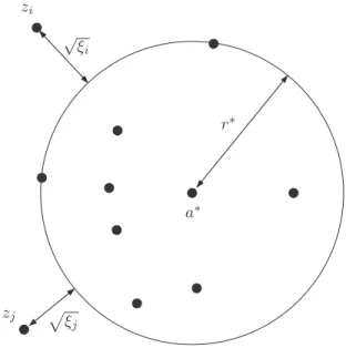
(17) with a parameter ν in ]0, 1] to control the trade-off between minimizing the radius and controlling the slack variables defined as ξi = (*a − zi*2− r2)+, see Fig. 6. The exact

role of ν will be discussed next.

We can solve this constrained optimization problem by defining a Lagrangian involving one Lagrange multiplier for each constraint: L(a, r, ξ; α, β) = r2+ J ! i=1 ξi/νJ + J ! i=1 αi(*zi− a*2− r2− ξi) − J ! i=1 βiξi, (18) with αi, βi ≥ 0. Setting to zero its derivatives with respect to

the primal variables a, r and ξ gives a∗=

J

!

i=1

α∗izi (19)

where α∗ is the solution of the optimization problem maxα 0Ji=1αi$zi, zi% −0Ji,j=1αiαj$zi, zj%

subject to 0J_i=1αi= 1, 0 ≤ αi≤ 1/νJ, i = 1, . . . , J.

(20) Depending on whether a training data zi lies inside the

hypersphere, on or outside, it can be shown that its Lagrange multiplier α∗

i in (19) satisfies one of the three conditions:

α∗

i = 0 (inside), 0 < α∗i < 1/νJ (on), and α∗i = 1/νJ

(outside). With condition 0J_i=1α∗

i = 1 in (20), we know

that there can be at most νJ training points lying outside the hypersphere. Furthermore, with the upper bound 1/νJ on α∗

i,

we observe that at least νJ training data do not lie inside the hypersphere.

After discussing the role of the parameter ν, which allows the user some control over the fraction of points that are excluded from the hypersphere, we shall now derive the

decision rule for novelty detection. The distance of any point x from the center a∗ _{of the hypersphere can be shown to be}

*x − a∗* = 1 2 2 3$x, x% − 2!J i=1 α∗ i$x, zi% + J ! i,j=1 α∗ iα∗j$zi, zj% (21) Equation (21) can be used to calculate the radius r∗ of the optimal hypersphere, that is, r∗ _{:= *z}

i0 − a∗* with i0 the

index of any training data such that 0 < α∗

i0 < 1/νJ. This

allows us to compute the resulting slack values ξi, see the

definition below equation (17). Consider now the test statistics Θ(x) := *x − a∗_*2

− (r∗₎2 _{such that the decision function}

d(x) :=

- _{1 if Θ(x) > γ : “nonstationarity";}

0 if Θ(x) < γ : “stationarity" (22) outputs 1 if the test point x lies outside the hypersphere of squared radius (r∗)2_{+ γ and so is considered novel, and 0}

otherwise. The threshold parameter γ has a direct influence upon the performance of the novelty detector. With probability greater than 1− δ, we can bound the probability that function d outputs 1 on a test point drawn according to the original distribution by [30] 1 γJ J ! i=1 ξi+ 6R2 γ√J + 3 4 ln(2/δ) 2J (23)

where R is the radius of a ball in feature space centered at the origin containing the support of the distribution. Such examples are false positives in the sense that they are normal data identified as novel by the decision function d. Obviously, we cannot bound the rate of true negatives since we have no way of guaranteeing what output d returns for data drawn from a different distribution. The strategy underlying this approach is however the smaller the hypersphere, the more likely novel data will fall outside and be identified as outlier.

When a more sophisticated model than the hypersphere is required to accurately fit the quantile functions, a pos-sible strategy is to replace each inner product _$zi, zj%

in equations (20)–(22) by a kernel function κ(zi, zj) :=

$φ(zi), φ(zj)%. An ideal kernel would implicitly map the

data via φ(_{·) into a bounded spherically-shaped area of a} new feature space. Kernel functions can usually be com-puted more efficiently as a direct function of the input data, without explicitly evaluating the mapping φ(_{·). Classic} exam-ples of kernels are the radially Gaussian kernel κ(zi, zj) =

exp$_−*zi− zj*2/2σ02

%

, and the Laplacian kernel κ(zi, zj) =

exp(−*zi− zj*/σ0), with σ0 ≥ 0 the kernel bandwidth.

Another example which deserves attention in signal processing is the q-th degree polynomial kernel defined as κ(zi, zj) =

(1 + $zi, zj%)q, with q ∈ N∗. In [32], we have extended the

framework of the so-called kernel-based methods to time-frequency analysis, showing that some specific reproducing kernels allow these algorithms to operate in the time-frequency domain. This link offers new perspectives in the field of non-stationary signal analysis, which can benefit from the developments of pattern recognition and statistical learning theory.

a∗ r∗ √ ξi & ξj zi zj

Fig. 6. Support vector data description algorithm

C. Testing stationarity

We shall now use support vector data description to estimate the support of probability density functions of stationary surrogate signals. The resulting decision rule will allow us to distinguish between stationary and nonstationary processes. Let us assume that we are given a training set {s1(t), . . . , sJ(t)} of surrogate signals generated from the

signal x(t) under investigation. In all the experiments reported above, time-frequency features were extracted from the nor-malized multitaper spectrogram of each signal, defined at time tn by Sn(f) := Sx,K (tn, f ) 0N n=1 /1 2 0 Sx,K(tn, f ) df (24) for n = 1, ..., N and 0≤ f < 1/2. More precisely, the local power Pn of each signal and its local frequency content Fn

summarized below were considered: Pn := # 1 2 0 Sn(f) df ; Fn := 1 Pn # 1 2 0 f Sn(f) df. (25)

Finally, for a sake of clarity, only the following two features comparing local time-frequency behavior to global one were retained

P := std(Pn)n=1,...,N ; F := std(Fn)n=1,...,N, (26)

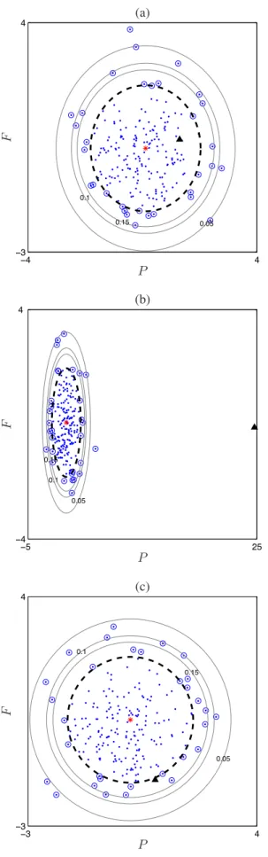
where std(_{·) denotes the standard deviation. The first one is} a measure of the fluctuations over time of the local power of the signal, whereas the second one operates the same way with respect to the local mean frequency. For each experiment reported in Fig. 7, a training set consisting of 200 surrogate signals was generated from the AM or FM signal x(t) to be tested. Features P and F were extracted from each signal. Next, data were mean-centered and normalized so that the variance of both features was one. Finally, the support vector data description algorithm was run using the basic linear kernel κ(zi, zj) = $zi, zj% and ν = 0.15. The results are displayed

for T0= T/20, T and 20 T , allowing to consider stationarity

relatively to the ratio between the observation time T and the modulation period T0. In each figure, the surrogate signals

are shown with dots and the signal to be tested with a black triangle. The optimum circle having center at c∗ _{and radius}

r∗ _{is shown in dashed line. The training data lying on or}

outside this circle, and thus associated with non-zero Lagrange multipliers in (19)-(21), are indicated by the circled dots. The thin circles represent the decision function (22) tuned to different false positive probabilities, fixed by γ via the relation (23). To calculate γ, note that we have neglected the contribution of the last two terms of equation (23) since they decay to zero as J tends to infinity. Figs. 7(b) and7(e) show that the test signals can be considered as nonstationary with a false positive probability lower than 0.05. In the other figures, they are clearly identified as stationary signals.

The findings reported in this learning-theory-based study are clearly consistent with what had been obtained previously with the distance-based approach. For a small modulation period or a large observation time, i.e., when T0 ) T , the situation

can be considered as stationary due to the observation of many similar oscillations over the observed time scale. This is reflected by the test signal which lies inside the region defined by the support vector data description algorithm for the stationary surrogates. For a medium observation time, i.e., T _{≈ T}0, the local evolution due to the modulation is prominent

and the black triangle for the modulated signal is well outside the stationary region, in accordance with a situation that can be referred to as nonstationary. Finally, if T0( T , the result turns

back to stationarity in the AM case because no significative change in the amplitude is observed over the considered time scale. In the FM case, the situation is slightly different, with the black triangle lying at the border of the surrogates domain. For the FM case, especially Figs. 7(e) and7(f), P is negative and lower than the values of P taken by the surrogates: this is characteristic of some regularity and constancy in the amplitude, which has less fluctuations than any corresponding stationary random process. Indeed, the way stationarity is tested cannot end up with a better configuration in this case since, by construction, surrogates of finite length pure tones undergo necessarily some amplitude fluctuations leading to a negative, non-zero P index for the (non-fluctuating) test signal. This can be viewed as a limitation of the method but it should rather be interpreted as a known bias when the test signal lies at the border of the surrogates domain and comes along with a value F close to 0. It could be used as an indication to discriminate random processes from more deterministic ones. Interestingly, one can also remark that the location of the test signal in the (P, F ) plane turns out to provide some information about the type of nonstationarity, if any: F ,= 0 is characteristic of some FM structure, P > 0 indicates some AM, P < 0 is associated to a constant (maybe deterministic) behavior for the amplitude (see [33] for preliminary results in this direction).

V. CONCLUSION

A new approach has been proposed for testing stationarity from a time-frequency viewpoint, relatively to a given observa-tion scale. A key point of the method is that the null hypothesis

of stationarity (which corresponds to time-invariance in the time-frequency spectrum) is statistically characterized on the basis of a set of surrogates which all share the same average spectrum as the analyzed signal while being stationarized. Two possible ways of making use of surrogates have been discussed, based either on a distance-based approach or on a machine learning technique (one class-SVM). Both ways are complementary since the first one is parametric whereas the second one is not. As is usual, a parametric approach based on a specific model for the distribution is naturally more efficient in terms of required data size, but it is based on the assumption that the underlying model is correct, something which has to be either known a priori or assessed. On the contrary, a non-parametric approach such as SVM does not require such assumptions, but it is more demanding in terms of data size and computation. Moreover, for the distance-based approach, some analytical studies can be conducted (possibly in asymptotic situations, see [34]), whereas the SVM approach allows for more versatile characterization of types of non-stationarity. As for comparing to early works using asymptotic analysis of evolutionary spectra [11], [12] to formulate a global test of stationarity, the assumption of independence between the frequency bins requires that many data in the time-frequency representations have to be discarded for the test. Our resampling method with surrogates allow for lightening this limitation and using all the bins, hence providing a method that uses all available information.

The basic principles of the method have been outlined, with a number of considerations related to its implementation, but it is clear that the proposed framework still leaves room for more thorough investigations as well as variations and/or extensions. In terms of time-frequency distributions for instance, one could imagine to go beyond spectrograms and take advantage of more recent advances [35]. Two-dimensional extensions can also be envisioned for testing stationarity in the sense of homogeneity of random fields, e.g., for texture analysis. Preliminary results in this direction are given in [36].

VI. ACKNOWLEDGMENTS

The authors thank Andrea Ferrari (from Laboratoire FIZEAU (UMR CNRS 6525), Observatoire de la Côte d’Azur, Université de Nice Sophia-Antipolis) for interesting discus-sions about statistics of surrogate data.

REFERENCES

[1] J. Xiao, P. Borgnat, and P. Flandrin, “Testing stationarity with time-frequency surrogates,” in Proc. EUSIPCO-07, Poznan (PL), 2007, pp. 2020–2024.

[2] J. Xiao, P. Borgnat, P. Flandrin, and C. Richard, “Testing stationarity with surrogates – A one-class SVM approach,” in Proc. IEEE Stat. Sig.

Proc. Workshop SSP-07, Madison (WI), 2007, pp. 720–724.

[3] S. Mallat, G. Papanicolaou, and Z. Zhang, “Adaptive covariance esti-mation of locally stationary processes,” Ann. of Stat., vol. 24, no. 1, pp. 1–47, 1998.

[4] W. Martin and P. Flandrin, “Detection of changes of signal structure by using the Wigner-Ville spectrum,” Signal Proc., vol. 8, pp. 215–233, 1985.

[5] R. Silverman, “Locally stationary random processes,” IRE Trans. on

Info. Theory, vol. 3, pp. 182–187, 1957.

[6] M. Davy and S. Godsill, “Detection of abrupt signal changes using Support Vector Machines: An application to audio signal segmentation,” in Proc. IEEE ICASSP-02, Orlando (FL), 2002, pp. 1313–1316.

[7] H. Laurent and C. Doncarli, “Stationarity index for abrupt changes detection in the time-frequency plane,” IEEE Signal Proc. Lett., vol. 5, no. 2, pp. 43–45, 1998.

[8] W. Martin, “Measuring the degree of non-stationarity by using the Wigner-Ville spectrum,” in Proc. IEEE ICASSP-84, San Diego (CA), 1984, pp. 41B.3.1–41B.3.4.

[9] S. Kay, “A new nonstationarity detector,” IEEE Trans. on Signal Proc., vol. 56, no. 4, pp. 1440–1451, 2008.

[10] P. Basu, D. Rudoy, and P. Wolfe, “A nonparametric test for stationarity based on local fourier analysis,” in Proc. IEEE ICASSP-09, Taiwan (ROC), 2009, pp. 3005–3008.

[11] M. B. Priestley and T. S. Rao, “A test for non-stationarity of time-series,”

Journal of the Royal Statistical Society. Series B (Methodological),

vol. 31, no. 1, pp. 140–149, 1969.

[12] M. B. Priestley, Non-linear and Non-stationaryTime Series Analysis. Academic Press, 1988.

[13] ——, “Evolutionary spectra and non-stationary processes,” Journal of

the Royal Statistical Society. Series B (Methodological), vol. 27, no. 2,

pp. 204–237, 1965.

[14] P. Flandrin, Time-Frequency / Time-Scale Analysis. Academic Press, 1999.

[15] M. Bayram and R. Baraniuk, “Multiple window time-varying spectrum estimation,” in Nonlinear and Nonstationary Signal Processing, W. F. et al., Ed. Cambridge Univ. Press, 2000.

[16] J. Theiler, S. Eubank, A. Longtin, B. Galdrikian, and J. D. Farmer, “Testing for nonlinearity in time series: the method of surrogate data,”

Physica D, vol. 58, no. 1–4, pp. 77–94, 1992.

[17] C. Keylock, “Constrained surrogate time series with preservation of the mean and variance structure,” Phys. Rev. E, vol. 73, pp. 030 767.1– 030 767.4, 2006.

[18] M. Basseville, “Distances measures for signal processing and pattern recognition,” Signal Proc., vol. 18, no. 4, pp. 349–369, 1989. [19] J. Xiao, P. Borgnat, and P. Flandrin, “Sur un test temps-fréquence

de stationnarité,” Traitement du Signal, 2009, (in French, with extended English summary, to appear). Preprint available from http://prunel.ccsd.cnrs.fr/ensl-00261530/.

[20] E. Serpedin, F. Panduru, I. Sari, and G. Giannakis, “Bibliography on cyclostationarity,” Signal Proc., vol. 85, no. 12, pp. 2233–2303, 2005. [21] P. J. Brockwell and R. A. Davies, Time series : theory and methods

(Second Edition). Springer series in statistics, 1991.

[22] Y. Dwivedi and S. S. Rao, “A test for second order stationarity of a time series based on the Discrete Fourier Transform,” arXiv:0911.4744, 2009.

[23] J. Huillery, F. Millioz, and N. Martin, “On the description of spectrogram probabilities with a Chi-squared law,” IEEE Transactions on Signal

Processing, vol. 56, no. 6, pp. 2249–2258, June 2008.

[24] E. Parzen, “On estimation of a probability density function and mode,”

Annals of Mathematical Statistics, vol. 33, no. 3, pp. 1065–1076, 1962.

[25] T. W. Sager, “An iterative method for estimating a multivariate mode and isopleth,” Journal of the American Statistical Association, vol. 74, no. 366, pp. 329–339, 1979.

[26] M. Moya, M. Koch, and L. Hostetler, “One-class classifier networks for target recognition applications,” in Proc. World Congress on Neural

Networks, 1993, pp. 797–801.

[27] M. Moya and D. Hush, “Network contraints and multi-objective opti-mization for one-class classification,” Neural Networks, vol. 9, no. 3, pp. 463–474, 1996.

[28] D. M. J. Tax and R. P. W. Duin, “Support vector data description,”

Machine Learning, vol. 54, no. 1, pp. 45–66, 2004.

[29] B. Schölkopf, J. C. Platt, J. Shawe-Taylor, A. J. Smola, and R. C. Williamson, “Estimating the support of a high-dimensional distribution,”

Neural Computation, vol. 13, no. 7, pp. 1443–1471, 2001.

[30] J. Shawe-Taylor and N. Cristianini, Kernel Methods for Pattern Analysis. Cambridge University Press, 2004.

[31] R. Vert, “Theoretical insights on density level set estimation, application to anomaly detection,” Ph.D. dissertation, Paris 11 - Paris Sud, 2006. [32] P. Honeiné, C. Richard, and P. Flandrin, “Time-frequency learning

machines,” IEEE Trans. on Signal Proc., vol. 55, no. 7 (Part 2), pp. 3930–3936, 2007.

[33] H. Amoud, P. Honeine, C. Richard, P. Borgnat, and P. Flandrin, “Time-frequency learning machines for nonstationarity detection using surrogates,” in Proc. IEEE Stat. Sig. Proc. Workshop SSP-09, Cardiff, (UK), 2009, pp. 565–568.

[34] C. Richard, A. Ferrari, H. Amoud, P. Honeine, P. Flandrin, and P. Borgnat, “Statistical hypothesis testing with time-frequency surrogates to check signal stationarity,” in Proc. IEEE ICASSP-10, Dallas (TX), 2010, p. to appear.

[35] J. Xiao and P. Flandrin, “Multitaper time-frequency reassignment for nonstationary spectrum estimation and chirp enhancement,” IEEE Trans.

on Signal Proc., vol. 55, no. 6 (Part 2), pp. 2851–2860, 2007.

[36] P. Borgnat and P. Flandrin, “Revisiting and testing stationarity,” J. Phys.:

Conf. Series., vol. 139, p. 012004, 2008.

Pierre Borgnat was born in Poissy, France, in 1974. He made his studies at the École Normale Supérieure de Lyon, France, receiving the Professeur-Agrégé de Sciences Physiques degree in 97, a Ms. Sc. in Physics in 99 and defended a Ph.D. degree in Physics and Signal Processing in 2002. In 2003-2004, he spent one year in the Signal and Image Processing group of the IRS, IST (Lisbon, Portugal). Since October 2004, he has been a full-time CNRS researcher with the Laboratoire de Physique, ÉNS Lyon. His research interests are in statistical signal processing of non-stationary processes (time-frequency representations, time deformations, stationarity tests) and scaling phenomena (time-scale, wavelets) for complex systems (turbulence, networks,...). He is also working on Internet traffic measurements and modeling, and in analysis and modeling of dynam-ical complex networks.

Patrick Flandrin (M’85–SM’01–F’02) received the engineer degree from ICPI Lyon, France, in 1978, and the Doct.-Ing. and “Docteur d’État” degrees from INP Grenoble, France, in 1982 and 1987, respectively. He joined CNRS in 1982, where he is currently Research Director. Since 1991, he has been with the “Signals, Systems and Physics” Group, within the Physics Department at École Normale Supérieure de Lyon, France. In 1998, he spent one semester in Cambridge, UK, as an invited long-term resident of the Isaac Newton Institute for Mathemat-ical Sciences and, from 2002 to 2005, he has been Director of the CNRS national cooperative structure “GdR ISIS.” His research interests include mainly nonstationary signal processing (with emphasis on time-frequency and time-scale methods) and the study of self-similar stochastic processes. He published many research papers in those areas and he is the author of the book Temps-Fréquence (Paris: Hermès, 1993 and 1998), translated into English as Time-Frequency/Time-Scale Analysis (San Diego: Academic Press, 1999). He has been a guest co-editor of the Special Issue “Wavelets and Signal Processing” of the IEEE TRANSACTIONS ONSIGNALPROCESSING

in 1993, the Technical Program Chairman of the 1994 IEEE-SP Int. Symp. on Time-Frequency and Time-Scale Analysis and, since 2001, he is the Program Chairman of the French GRETSI Symposium on Signal and Image Processing. He is currently an Associate Editor for the IEEE TRANSACTIONS ONSIGNAL

PROCESSING, and he has been a member of the “Signal Processing Theory and Methods” Technical Committee of the IEEE Signal Processing Society from 1993 to 2004.

Dr. Flandrin was awarded the Philip Morris Scientific Prize in Mathematics in 1991, the SPIE Wavelet Pioneer Award in 2001 and the Prix Michel Monpetit from the French Academy of Sciences in 2001. He is Fellow of IEEE (2002) and of EURASIP (2009).

Paul Honeine (M’07) was born in Beirut, Lebanon, on October 2, 1977. He received the Dipl.-Ing. degree in mechanical engineering in 2002 and the M.Sc. degree in industrial control in 2003, both from the Faculty of Engineering, the Lebanese University, Lebanon. In 2007, he received the Ph.D. degree in Systems Optimisation and Security from the Uni-versity of Technology of Troyes, France, and was a Postdoctoral Research associate with the Systems Modeling and Dependability Laboratory, from 2007 to 2008. Since September 2008, he has been an assis-tant Professor at the University of Technology of Troyes, France. His research interests include nonstationary signal analysis, nonlinear adaptive filtering, sparse representations, machine learning, and wireless sensor networks. He is the co-author (with C. Richard) of the 2009 Best Paper Award at the IEEE Workshop on Machine Learning for Signal Processing.

CÈdric Richard (S’98–M’01–SM’07) was born January 24, 1970 in Sarrebourg, France. I received the Dipl.-Ing. and the M.S. degrees in 1994 and the Ph.D. degree in 1998 from the University of Technology of CompiËgne, France, all in Electrical and Computer Engineering. From 1999 to 2003, he was an Associate Professor at the University of Technology of Troyes, France. From 2003 to 2009, he was a Full Professor at the Institut Charles Delaunay (CNRS FRE 2848) at the UTT, and the supervisor of a group consisting of 60 researchers and Ph.D. In winter 2009, he was a Visiting Researcher with the Department of Electrical Engineering, Federal University of Santa Catarina (UFSC), FlorianÚpolis, Brazil.

Since September 2009, CÈdric Richard is a Full Professor at Fizeau Laboratory (CNRS UMR 6525, Observatoire de la CÙte d’Azur), University of Nice Sophia-Antipolis, France. His current research interests include statistical signal processing and machine learning. Prof. CÈdric Richard is the author of over 100 papers. He was the General Chair of the XXIth francophone conference GRETSI on Signal and Image Processing that was held in Troyes, France, in 2007. Since 2005, he is in charge of the Ph.D. students network of the federative CNRS research group ISIS on Information, Signal, Images and Vision. He is a member of GRETSI association board and of the EURASIP society, and Senior Member of the IEEE.

Cédric Richard serves as an Associate Editor of the IEEE Transactions on Signal Processing since 2006, and of the EURASIP Signal Processing Magazine since 2009. In 2009, he was nominated liaison local officer for EURASIP, and member of the Signal Processing Theory and Methods (SPTM) Technical Committee of the IEEE Signal Processing Society.

Paul Honeine and Cédric Richard received Best Paper Award for “Solving the pre-image problem in kernel machines: a direct method” at the 2009 IEEE Workshop on Machine Learning for Signal Processing (IEEE MLSP’09).

Jun Xiao received the B.E. degree in opto-electronics and the M.S. degree in optics (with highest honors) from East China Normal University, PRC, in 2002 and 2005, respectively. She received in 2008 a Ph.D. degree in Signal Processing from École Normale Supérieure de Lyon (France) and East China Normal University, Shanghai (PRC).

−4 4 −3 4 0.05 0.1 0.15 (a) F P −3 4 −3 4 0.05 0.1 0.15 (d) F P −5 25 −4 4 0.05 0.1 0.15 (b) F P −4 3 −4 10 0.05 0.10.15 (e) F P −3 4 −3 4 0.05 0.1 0.15 (c) F P −4 4 −3 4 0.05 0.1 0.15 (f) F P

Fig. 7. Time-frequency features (P, F ) in AM (left) and FM (right) situations. From top to bottom, T0= T /20, T and 20 T , with T = 1600. In each case,

the black triangle corresponds to the (P, F ) pair of one test signal used to derive the surrogates. The latter are plotted as dots which, with support vector data description, define the minimum-volume domain of stationarity represented here by the dashed curve. The training data lying on or outside this area are indicated by the circled dots. The thin curves represent the decision functions with false positive probabilities 0.05, 0.1 and 0.15. Other parameters are as follows — number of tapers: K = 5, length of tapers: Th= 387, modulation indices: (AM) m = 0.5 and (FM) m = 0.02, central frequency f0= 0.25,