Compromis espace-temps pour le problème de k plus courts chemins simples

HAL Id: hal-02835953

https://hal.inria.fr/hal-02835953

Submitted on 7 Jun 2020

HAL is a multi-disciplinary open access

archive for the deposit and dissemination of

sci-entific research documents, whether they are

pub-lished or not. The documents may come from

teaching and research institutions in France or

abroad, or from public or private research centers.

L’archive ouverte pluridisciplinaire HAL, est

destinée au dépôt et à la diffusion de documents

scientifiques de niveau recherche, publiés ou non,

émanant des établissements d’enseignement et de

recherche français ou étrangers, des laboratoires

publics ou privés.

Compromis espace-temps pour le problème de k plus

courts chemins simples

Ali Al Zoobi, David Coudert, Nicolas Nisse

To cite this version:

Ali Al Zoobi, David Coudert, Nicolas Nisse. Compromis espace-temps pour le problème de k plus

courts chemins simples. ALGOTEL 2020 – 22èmes Rencontres Francophones sur les Aspects

Algo-rithmiques des Télécommunications, Sep 2020, Lyon, France. pp.4. �hal-02835953�

de k plus courts chemins simples

†‡

Ali Al Zoobi

1

et David Coudert

1

et Nicolas Nisse

1

1_{Universit´e Cˆote d’Azur, Inria, CNRS, I3S, France}

Le probl`eme de trouver k plus courts chemins simples (sans r´ep´etition de sommets) entre deux sommets dans un graphe a ´et´e largement ´etudi´e du point de vue de l’ing´enierie algorithmique. Kurz et Mutzel (2016) ont propos´e l’algorithme SB (pour Sidetrack Based) bas´e sur le concept de d´eviations, qui est actuellement la m´ethode la plus rapide en pratique. Dans ce travail, nous proposons deux am´eliorations de cet algorithme. Nous montrons tout d’abord comment acc´el´erer l’algorithme SB en utilisant des mises `a jour dynamiques d’arbres de plus courts chemins. Nos simulations r´ealis´ees sur certains r´eseaux routiers avec environ un demi-million de sommets et un million d’arcs montrent que notre am´elioration donnent une acc´el´eration moyenne d’un facteur 1,5 `a 2 avec une consommation de m´emoire similaire `a celle de l’algo-rithme SB. Notre principale contribution est un second algol’algo-rithme r´ealisant un compromis entre temps d’ex´ecution et m´emoire utilis´ee. Notre algorithme permet de r´eduire significativement la m´emoire de travail (d’un facteur 1, 5 `a 2) au prix d’une l´eg`ere augmentation du temps d’ex´ecution.

Mots-clefs : k plus courts chemins simples, algorithmes de graphes, compromis complexit´e espace-temps

1

Introduction

The classical k shortest paths problem (kSP) returns the top-k shortest paths (SP) between a source and a destination in a digraph. This problem has numerous applications in various kinds of networks (road and transportation networks, communications networks, social networks, etc.) and is also used as a building block for solving optimization problems. Let D = (V, A) be a digraph with n vertices and m arcs, and with a weight function ω : A → R+on its arcs. A (directed) s-t path is a sequence (s = v0, v1, · · · , vl = t) of

vertices starting from s and ending at t, such that (vi, vi+1) ∈ A for all 0 ≤ i < l. It is called simple if it has

no repeated vertices, i.e., vi6= vjfor all 0 ≤ i < j ≤ l. The weight of a path is the sum of the weights of its

arcs and the distance dD(u, v) between two vertices u, v ∈ V is the minimum weight of a u-v path in D. A set

P

of s-t paths is a top-k set of s-t paths if |

P

| = k and no s-t path not in

P

has weight strictly less than some path in

P

. Eppstein’s algorithm [Epp98] has the best time-complexity, O(m + n log n + k), for this problem. An important variant of this problem is the k shortest simple paths problem (kSSP) which adds the constraint that reported paths must be simple. The algorithm with the best known time complexity for solving the kSP problem has been proposed by Yen [Yen71], with time complexity in O(kn(m + n log n)). Since, several proposals have been made to improve the practical efficiency of the algorithm [Fen14,KM16]. Recently, Kurz and Mutzel [KM16] obtained a tremendous practical running time improvement. The key idea of their Sidetrack Based (SB) algorithm was to postpone as much as possible the computation of trees that are done earlier by Yen’s algorithm. We present a slight improvement of SB algorithm and a modification of it allowing to establish a tradeoff between the running time and the memory consumption. Our contribution. Section 2 presents Kurz and Mutzel’s SB algorithm with a particular attention to the used data structures. This allows us, in Section 3, to describe a first slight improvement, using dynamic updates of shortest path trees, and resulting to a notable speed up of SB algorithm, with an average speed up by a factor of 1.5 to 2 and with a similar working memory consumption. Our main contribution, presented in Section 3, is a more involved adaptation of the SB algorithm, enabling to significantly reduce the working memory (with a factor of 1.5 to 2) at the cost of a small increase of the running time. We conclude with the results of our simulations comparing the performances of our algorithms with the previous ones.

†_{The full version of this paper can be found here: https://hal.archives-ouvertes.fr/hal-02465317.}

‡_{This work has been supported by the UCA}JEDI

Investments in the Future project managed by the National Research Agency (ANR-15-IDEX-01), project MULTIMOD (ANR-17-CE22-0016), project Digraphs (ANR-19-CE48-0013), and by R´egion Sud PACA.

Ali Al Zoobi et David Coudert et Nicolas Nisse

2

Kurz and Mutzel’s algorithm

We give a short presentation of Kurz and Mutzel’s Sidetrack Based (SB) algorithm in order to explain our contributions in the next section. Let (D = (V, A), ω) be an arc-weighted digraph, s,t ∈ V and k ∈ N. The goal of SB algorithm is to compute a top-k set

P

of simple shortest s-t paths (assuming they exist). Compact representation of a path. The SB algorithm is based on a data structure generalizing the repre-sentation of a path proposed by Eppstein [Epp98]. Let us present this data structure briefly below.

An in-branching T rooted at t is a sub-digraph of D that induces a tree containing t and such that every u∈ V (T ) \ {t} has exactly one out-neighbor (that is, all paths in T go toward t) and, for every u ∈ V (T ), the weight of the (unique) u-t path Put(T ) in T equals dD(u,t), i.e, Put(T ) is a shortest u-t path (both in T and

D). Let P = (v0, v1, · · · , vr) be any path in D and i < r. Any arc a = viw6= vivi+1is called a deviation of P

at vi. Any path Q = (v0, · · · , vi, w, w1, · · · , w`= t) where w, w1, · · · , w`= t is a shortest wt path in D is called

an extension of P at a (or at vi). Note that neither P nor Q is required to be simple.

Kurz and Mutzel’s proposed a compact representation of paths using sequences of in-branchings and deviations. Precisely, the sequence ε = (T0, e0, T1, e1, · · · , Th, eh, Th+1) (with ei= (vi, wi) for all i ≤ h)

repre-sents the path P starting at s, following T0until the tail v0of e0, then the deviation e0, then T1until it reaches

the tail v1 of e1, etc. until it reaches the head whof eh, plus (possibly) a path from wh to t in Th+1. That

is, P is the sequence of vertices of the paths Psv0(T0), Pw0v1(T1), · · · , Pwh−1vh(Th) followed by the vertices of

Pwht(Th+1) if this latter path exists. Two consecutive in-branchings Tiand Ti+1are not necessarily distinct.

SB algorithm ensures that, if P is an s-t path (i.e., if Pwht(Th+1) exists), then the subpath Pre f of P going

from s to wh(v0, · · · , wh) is always simple and P is not simple only if Pwht(Th+1) intersects Pre f .

Sidetrack Based (SB) Algorithm. We are now ready to present SB algorithm. Roughly, SB algorithm uses a set

C

to manage candidate paths that are encoded using the above data structure. Sequentially, it extracts a shortest element ε from

C

. If ε represents a simple path P, this path is added to the output

P

and the representations of its extensions are computed and added to

C

. Otherwise, SB algorithm attempts to modify ε by instantiating its last in-branching (this is one bottleneck both for the time and space complexities since an in-branching is actually computed by applying Dijkstra’s algorithm, and is stored). If this computation leads to the representation of a simple path, then it is added to

C

. Otherwise, ε is discarded. SB algorithm goes on iteratively until it has found k paths. The initialisation consists in computing a first in-branching T0

in D (using Dijkstra’s alg.) and so a shortest s-t (simple) path Pst(T0) and adding its representation to

C

.

More precisely, the set

_C

is a min-heap in which the weight of an element is a lower bound on the weight of the path it represents. Each element µ in

C

has the form µ = (ε = (T0, e0, · · · , eh= (vh, wh), Th+1), lb, ζ)

where each in-branching T_h0 (with h0≤ h) is already computed and lb is a lower bound of the weight of the

path represented by ε. The value ζ is a boolean indicating whether the path represented by ε is known to be simple. If so, it will follow from the construction that Th+1has already been computed, else Th+1must be

first computed to know if ε represents a simple path. For the initialization, the in-branching T0is computed

and the element ((T0), ω(Pst(T0)), ζ = 1) is inserted in

C

.

SB algorithm iteratively extracts elements from

C

by minimum weight (with a priority to representa-tion of simple paths to break ties) until k paths are obtained or

C

is empty. When an element µ = (ε = (T0, e0, · · · , eh= (vh, wh), Th+1), lb, ζ) is extracted from

C

, two cases are distinguished :

Case ζ = 1. Then, ε represents a simple path P = (v0= s, · · · , vi= wh, · · · , vr= t) and all the in-branchings

Ti’s have already been computed. In this case, the path P is added to the output

P

. Then, for every

i≤ j < r, and for every deviation e = (vj, w) at vj, let Pwt(Th+1) be the shortest path from w to t in Th+1

and let Q(vj, e) = (v0, · · · , vj, w, Pwt(Th+1)). If Q(vj, e) is simple (this can be verified efficiently using

a trick of Feng [Fen14]), the representation µ0= ((T0, e0, · · · , eh, Th+1, e = (vj, w), Th+1), lb(e), ζ = 1)

is added to

C

with lb(e) = ω(Q(vj, e)) as a key (note that the computation of lb(e) is done in

constant time since, in particular, Th+1 is already computed). Otherwise (Q(vj, e) is not simple),

the representation µ00= (ε00= (T0, e0, · · · , eh, Th+1, e = (vj, w), T0), lb(e), ζ = 0) is added to

C

, where

T0 is the name of the in-branching of D \ {v0, · · · , vj} whose actual computation is postponed, and

lb(e) = ω(Q(vj, e)) is a lower bound on the weight of the path represented by ε00.

Case ζ = 0. In this case, the algorithm checks for the existence of a wh-t path Pwt(Th+1). To do so,

in-branching in D \ {v0, · · · , vh}, which ensures that, if Pwt(Th+1) is found, the path Pnew= (s =

v0, · · · , vh, Pwht(Th+1)) is guaranteed to be simple. Moreover, Pnew has weight ω(Pnew) = ω((s =

v0, · · · , vh, wh)) + ω(Pwht(Th+1)). Then, the representation µ

0_{= (ε}0_{= (T}

0, e0, · · · , eh= (vh, wh), Th+1),

ω(Pnew), ζ = 1) is added to

C

. Finally, if no wh-t path can be found in Th+1, µ is discarded.

So far, SB algorithm has out-performed all other algorithms for solving the k-Shortest Simple Paths problem in terms of running time (e.g., it is ten times faster than Feng’s algorithm [Fen14] in large networks). Ho-wever, it has the drawback to have an important consumption of working memory (much more than Feng’s algorithm that stores a single in-branching, while keeping the whole description of paths it computes).

3

Our Contributions

SB* Algorithm. First, we propose a slight modification of SB algorithm (called SB*). Precisely, each time a representation (T0, e0, T1· · · , eh−1= (uh−1, vh−1), Th, eh= (uh, vh), Th+1) of a non simple path is extracted

from

C

with Th+1not computed yet (i.e., it is only a name), while SB algorithm computes Th+1from scratch

our algorithm does not. Instead, SB* algorithm creates a copy T of Th, discards vertices of the path from

vh−1to uhin Th, and updates the in-branching T using standard methods for updating an in-branching.Then,

the name Th+1is instantiated as the new in-branching T . It is clear that SB* algorithm computes (and store)

exactly the same number of in-branchings as SB algorithm. As demonstrated by the simulations below, SB* algorithm is up to twice faster than SB algorithm with the same memory consumption.

Parsimonious SB Algorithm. Now, let us present our main algorithm, called PSB, which is an adaptation of SB algorithm allowing to reduce the memory consumption due to the storage of all in-branchings computed by SB algorithm. Here, we only focus on the differences between SB and PSB algorithms.

The main difference is that PSB algorithm stores two types of elements in

C

. The first type, of the form (ε = (T0, e0, T1, e1, · · · , Th, eh= (vh, wh), Th+1), lb), represents a simple s-t path P of weight lb. Contrary

to SB algorithm, the in-branching Th+1 has not necessarily been computed yet. The second type, of the

form (ε, Dev, lb), contains an extra field Dev (explained below) and, in this case, all of the in-branchings T1, · · · , Th+1are already computed.

Let us start considering a step of PSB algorithm when an element µ = (ε = (T0, e0, T1, e1, · · · , Th, eh=

(vh, wh), Th+1), lb) representing a simple path P is extracted from

C

. Th+1is computed at this step (if not

already done) which allows to output P. Then, PSB algorithm adds P = (s = v0, · · · , vi= wh, · · · , vr= t) to

P

and (as SB algorithm) for every v ∈ {vi, · · · , vr}, and every deviation e with tail v, the extension Q(v, e)

is considered. If Q(v, e) is simple (again, checking whether an extension is simple or not is done using the trick of Feng), then µ0= ((T0, e0, T1, e1, · · · , Th, eh, Th+1, e, Th+1), ω(Q(v, e))) is added to

C

. Otherwise, the

deviation e is added to a set Dev (initially empty). Once all deviations have been considered, the (unique) element (ε, Dev, lb0) is added to

C

, where lb0= minfj=(uj,u0j)∈Devω(Q(uj, fj)). That is, Dev is the set of all

“non simple deviations” of P at the vertices between whand t, and lb0is a lower bound on the weight of the

extensions at a deviation in Dev. The important difference between SB and PSB algorithms comes from the fact that non simple extensions are considered as a unique object by PSB.

Now, let us consider a step when PSB algorithm extracts an element µ = (ε = (T0, e0, T1, e1, · · · , Th, eh, Th+1),

Dev= { f₁, · · · , f_j= (u_j, u0_j), · · · , f_l}, lb) from

C

. As mentioned above, in this case, ε encodes a simple s-t path (v0, · · · , vr). Let 1 ≤ min ≤ l be the smallest integer such that lb = ω(Q(umin, fmin)). Then, PSB

algo-rithm proceeds as follows. For j decreasing from l to min, an in-branching T_j0 in D \ {v0, · · · , vij = uj} is

computed (but not stored !) until a path P_u0 jt(T

0

j) from u0jto t is discovered (if no such path exists, j is

decrea-sed by one). If P_u0 jt(T

0

j) exists, then εj= (T0, e0, T1, e1, · · · , Th, eh, Th+1, fj, Tj0) represents a simple s-t path of

weight lbj= ω((v0, · · · , vij)) + ω( fj) + ω(Pu0_jt(Tj0)). Then, the element µj= (εj, lbj) is added to

C

, but Tj0

is not stored (PSB algorithm might have to recompute it later). A 2nd _{key improvement is that to speed up}

the computation, T_j0is actually computed by updating T_j+10 .Then, only when j = min, the in-branching T_min0 is stored and µmin= (εmin, lbmin) is added to

C

. The reason why Tmin0 is stored (while other T

0

j are not) is that

µminis expected to be extracted soon from

C

(because the path represented by εminis expected to be short)

and we want to avoid the recomputation of T_min0 . Finally, the element µ0= (ε, Dev0= { f1, · · · , fmin−1}, lb0)

Ali Al Zoobi et David Coudert et Nicolas Nisse

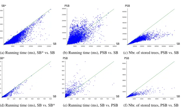
(a) Running time (ms), SB* vs. SB (b) Running time (ms), PSB vs. SB (c) Nbr. of stored trees, PSB vs. SB

(d) Running time (ms), SB vs. SB* (e) Running time (ms), SB vs. PSB (f) Nbr. of stored trees, PSB vs. SB

FIGURE1:Comparison of the running time of SB versus SB* (Fig. 1a) and SB versus PSB (Fig. 1b) on Rome (resp.

Fig. 1d and Fig. 1e on Colorado), and comparison of the number of stored trees for SB versus PSB (Fig. 1c) on Rome, (resp. Fig. 1f on Colorado). Each dot corresponds to one pair source/destination, among 1 000 randomly chosen pairs.

The correctness follows from the one of the SB algorithm. Moreover, since most of the computed in-branchings are not stored, the working memory used by PSB is significantly smaller than for SB algorithm. Experimental evaluation. We have implemented the algorithms SB, SB* and PSB in C++ and our code is publicly available athttps://gitlab.inria.fr/dcoudert/k-shortest-simple-paths. We have evaluated the performances of these algorithms on several road networks [DGJ]. Here we present the ones in a “small” network (Rome, n = 3 353, m = 8 870) and in a “large” one (Colorado, n = 435 666, m = 1 057 066). All computations have been done on a computer equipped with 2 quad-core 3.20GHz Intel Xeon W5580 processors and 64GB of RAM. Our simulations show that our improvement SB* of SB algorithm allows to decrease the running-time by a factor between 1,5 and 2 in average. In particular, for both networks, SB* algorithm is, for most of the queries, faster than SB algorithm (Figures (1a) and (1d)). The simulations comparing PSB and SB algorithms show a significant reduction of the working memory (number of stored trees) when using PSB (Figures (1c) and (1f)). In term of running time, SB algorithm is slightly faster in average but Figures (1b) and (1e) indicate that globally, they are quite comparable. Conclusion. To obtain a better tradeoff between space and time, a future work consist in determining a threshold τ such that an in-branching T is stored only if it is used to extract a path with weight at most τ.

R ´ef ´erences

[DGJ] C. Demetrescu, A. Goldberg, and D. Johnson. 9th dimacs implementation challenge - shortest paths. [Epp98] D. Eppstein. Finding the k shortest paths. SIAM Journal on Computing, 28(2) :652–673, 1998.

[Fen14] G. Feng. Finding k shortest simple paths in directed graphs : A node classification algorithm. Networks, 64(1) :6–17, 2014.

[KM16] D. Kurz and P. Mutzel. A sidetrack-based algorithm for finding the k shortest simple paths in a directed graph. In Int. Symp. on Alg. and Comp. (ISAAC), volume 64 of LIPIcs, pages 49 :1–49 :13, 2016.