Publisher’s version / Version de l'éditeur:
The Astrophysical Journal Supplement Series, 235, 1, 2018-02-16
READ THESE TERMS AND CONDITIONS CAREFULLY BEFORE USING THIS WEBSITE. https://nrc-publications.canada.ca/eng/copyright
Vous avez des questions? Nous pouvons vous aider. Pour communiquer directement avec un auteur, consultez la
première page de la revue dans laquelle son article a été publié afin de trouver ses coordonnées. Si vous n’arrivez pas à les repérer, communiquez avec nous à [email protected].
Questions? Contact the NRC Publications Archive team at
[email protected]. If you wish to email the authors directly, please see the first page of the publication for their contact information.
NRC Publications Archive
Archives des publications du CNRC
This publication could be one of several versions: author’s original, accepted manuscript or the publisher’s version. / La version de cette publication peut être l’une des suivantes : la version prépublication de l’auteur, la version acceptée du manuscrit ou la version de l’éditeur.
For the publisher’s version, please access the DOI link below./ Pour consulter la version de l’éditeur, utilisez le lien DOI ci-dessous.
https://doi.org/10.3847/1538-4365/aaa762
Access and use of this website and the material on it are subject to the Terms and Conditions set forth at
Where is OH and does it trace the dark molecular gas (DMG)?
Li, Di; Tang, Ningyu; Nguyen, Hiep; Dawson, J. R.; Heiles, Carl; Xu, Duo;
Pan, Zhichen; Goldsmith, Paul F.; Gibson, Steven J.; Murray, Claire E.;
Robishaw, Tim; Mcclure-Griffiths, N. M.; Dickey, John; Pineda, Jorge;
Stanimirović, Snežana; Bronfman, L.; Troland, Thomas
https://publications-cnrc.canada.ca/fra/droits
L’accès à ce site Web et l’utilisation de son contenu sont assujettis aux conditions présentées dans le site LISEZ CES CONDITIONS ATTENTIVEMENT AVANT D’UTILISER CE SITE WEB.
NRC Publications Record / Notice d'Archives des publications de CNRC:
https://nrc-publications.canada.ca/eng/view/object/?id=9deb0e83-ec17-47de-b69a-fe4fce507710 https://publications-cnrc.canada.ca/fra/voir/objet/?id=9deb0e83-ec17-47de-b69a-fe4fce507710Where is OH and Does It Trace the Dark Molecular Gas (DMG)?
Di Li1,2,3 , Ningyu Tang1 , Hiep Nguyen4,5, J. R. Dawson4,5 , Carl Heiles6, Duo Xu1,3,7, Zhichen Pan1, Paul F. Goldsmith8 , Steven J. Gibson9 , Claire E. Murray10,11 , Tim Robishaw12, N. M. McClure-Griffiths13 , John Dickey14 , Jorge Pineda8 ,
Snežana Stanimirović10, L. Bronfman15 , and Thomas Troland16 The PRIMO Collaboration17
1
National Astronomical Observatories, CAS, Beijing 100012, Peopleʼs Republic of China;[email protected],[email protected]
2
Key Laboratory of Radio Astronomy, Nanjing, Chinese Academy of Science, Peopleʼs Republic of China 3
University of Chinese Academy of Sciences, Beijing 100049, Peopleʼs Republic of China 4
Department of Physics and Astronomy and MQ Research Centre in Astronomy, Astrophysics and Astrophotonics, Macquarie University, NSW 2109, Australia 5
Australia Telescope National Facility, CSIRO Astronomy and Space Science, P.O. Box 76, Epping, NSW 1710, Australia 6
Department of Astronomy, University of California, Berkeley, 601 Campbell Hall 3411, Berkeley, CA 94720-3411, USA 7
Department of Astronomy, The University of Texas at Austin, Austin, TX 78712, USA 8
Jet Propulsion Laboratory, California Institute of Technology, 4800 Oak Grove Drive, Pasadena, CA 91109, USA 9
Western Kentucky University, Dept. of Physics and Astronomy, 1906 College Heights Boulevard, Bowling Green, KY 42101, USA 10
University of Wisconsin, Department of Astronomy, 475 N Charter Street, Madison, WI 53706, USA 11Space Telescope Science Institute, 3700 San Martin Drive, Baltimore, MD 21218, USA 12
Dominion Radio Astrophysical Observatory, National Research Council, P.O. Box 248, Penticton,BC, V2A 6J9, Canada 13
Research School for Astronomy & Astrophysics, Australian National University, Canberra, ACT 2611, Australia 14
University of Tasmania, School of Maths and Physics, Hobart, TAS 7001, Australia 15
Departamento de Astronomía, Universidad de Chile, Casilla 36, Santiago de Chile, Chile 16
Department of Physics and Astronomy, University of Kentucky, Lexington, Kentucky 40506, USA
Received 2017 November 3; revised 2018 January 8; accepted 2018 January 10; published 2018 February 16
Abstract
Hydroxyl (OH) is expected to be abundant in diffuse interstellar molecular gas because it forms along with H2under similar conditions and forms within a similar extinction range. We have analyzed absorption
measurements of OH at 1665 MHz and 1667 MHz toward 44 extragalactic continuum sources, together with the
J=1–0 transitions of12CO,13CO, and C18O, and the J=2–1 transition of12CO. The excitation temperatures of OH were found to follow a modified lognormal distribution f Tex 21 exp lnTex 2ln 3.4 K ,
2 2
µ p s ⎡⎣- -s ⎤⎦
( ) [ ( ) ( )] the peak of
which is close to the temperature of the Galactic emission background (CMB+synchrotron). In fact, 90% of the OH has excitation temperatures within 2 K of the Galactic background at the same location, providing a plausible explanation for the apparent difficulty of mapping this abundant molecule in emission. The opacities of OH were found to be small and to peak around 0.01. For gas at intermediate extinctions (AV∼ 0.05–2 mag), the detection
rate of OH with a detection limit N(OH);1012
cm−2is approximately independent of A
V. We conclude that OH is
abundant in the diffuse molecular gas and OH absorption is a good tracer of “dark molecular gas (DMG).” The measured fraction of DMG depends on the assumed detection threshold of the CO data set. The next generation of highly sensitive low-frequency radio telescopes, such as FAST and SKA, will make feasible the systematic inventory of diffuse molecular gas through decomposing, in velocity, the molecular (e.g., OH and CH) absorption profiles toward background continuum sources with numbers exceeding what is currently available by orders of magnitude.
Key words:evolution – ISM: clouds – ISM: molecules Supporting material: figure set
1. Introduction
The two relatively denser phases of the interstellar medium (ISM) are the atomic cold neutral medium (CNM) traced by the HI λ 21 cm hyperfine structure line and the “standard”
molecular (H2) clouds, usually traced by CO. CO has
historically been the most important tracer of molecular hydrogen, which remains largely invisible due to its lack of emission at temperatures in the molecular ISM. Empirically, CO intensities have been used as an indicator of the total molecular mass in the Milky Way and external galaxies through the so-called “X-factor,” with numerous caveats, not least of which is the large opacities of CO transitions. Gases in these two phases dominate the masses of star-forming clouds
on a galactic scale. The measured ISM gas mass from HIand CO is thus the foundation of many key quantities for understanding galaxy evolution and star formation, such as the star formation efficiency.
A growing body of evidence, however, indicates the existence of gas traced by neither HI nor CO. Comparative studies (e.g., de Vries et al. 1987) of Infrared Astronomy Satellite (IRAS) dust images and gas maps in HI and CO revealed an apparent “excess” of dust emission. The Planck Collaboration et al. (2011)clearly showed excess dust opacity in the intermediate extinction range AV∼0.05–2 mag,
roughly corresponding to the self-shielding thresholds of H2and 13CO, respectively. The missing gas, or rather, the
undetected gas component, is widely referred to as dark gas, popularized as a common term by Grenier et al. (2005). These
The Astrophysical Journal Supplement Series,235:1 (15pp), 2018 March https://doi.org/10.3847/1538-4365/aaa762
© 2018. The American Astronomical Society. All rights reserved.
17
Pacific Rim Interstellar Matter Observers;http://ism.bao.ac.cn/primo.
authors found more diffuse gamma-ray emission observed by the Energetic Gamma Ray Experiment Telescope (EGRET) than can be explained by cosmic ray interactions with the observed H-nuclei. Observations of the THz fine structure C+ line also helped reveal the dark gas, from which the C+line strength is stronger than can be produced by only HI gas (Langer et al.2010; Pineda et al.2013; Langer et al.2014). A minority within the ISM community has argued that dark gas can be explained by underestimated HIopacities (Fukui et al.
2015), which is in contrast with some other recent works (Stanimirović et al.2014; Lee et al.2015). We focus here on the dark molecular gas (DMG), more specifically CO-dark molecular gas.
ISM chemistry and PDR models predict the existence of H2in regions where CO is not detectable (Wolfire et al.2010).
CO can be have low abundance due to photodissociation in unshielded regions and/or can be heavily subthermal due to low collisional excitation rates in the diffuse gas. OH, or hydroxyl, was the first interstellar molecule detected at radio wavelengths (Weinreb et al. 1963). It can form efficiently through relatively rapid routes, including charge-exchange reactions initiated by cosmic ray ionization once H2becomes
available (van Dishoeck & Black1988). Starting from H+,
O H O H, O H2 OH H. 1 + + + + + + + + ( )
Also starting from H2+,
H H H H, H O OH H . 2 2 2 3 3 2 + + + + + + + + ( )
OH+then reacts with H2to form H2O +
, which continues onto H3O + , OH H H O H, H O H H O H. 3 2 2 2 2 3 + + + + + + + + ( ) H2O + and H3O +
recombine with electrons to form OH. OH can join the carbon reaction chain through reaction with C+and eventually produce CO,
OH C CO H, CO H HCO H, HCO e CO H. 4 2 + + + + + + + + + + + - ( )
Widespread and abundant OH, along with HCO+and C+, is thus expected in diffuse and intermediate extinction regions.
OH has been widely detected throughout the Galactic plane (e.g., Caswell & Haynes 1975; Turner 1979; Boyce & Cohen 1994; Dawson et al. 2014; Bihr et al. 2015), in local molecular clouds (e.g., Sancisi et al. 1974; Wouterloot & Habing 1985; Harju et al. 2000), and in high-latitude translucent and cirrus clouds (e.g., Grossmann et al. 1990; Barriault et al. 2010; Cotten et al. 2012). Crucially, a small number of studies have confirmed OH extending outside CO-bright regions (Wannier et al.1993; Liszt & Lucas1996; Allen et al. 2012, 2015), and/or associated with narrow HI
absorption features (Dickey et al. 1981; Liszt & Lucas 1996; Li & Goldsmith 2003), confirming its viability as a dark gas tracer. OH and HCO+have been shown to be tightly correlated in absorption measurements against extragalactic continuum sources (Liszt & Lucas 1996; Lucas & Liszt1996).
Because OH in emission is typically very weak, large-scale OH maps remain rare, particularly for diffuse molecular gas, which should presumably be dominated by DMG. Detectability often hinges on the presence of a bright continuum background against which the OH lines can be seen in absorption: either the bright diffuse emission of the inner Galactic plane (e.g., Dawson et al.2014)or bright, compact extragalactic/Galactic sources (e.g., Goss1968; Nguyen-Q-Rieu et al.1976; Crutcher
1977,1979; Dickey et al. 1981; Colgan et al. 1989; Liszt & Lucas1996). This latter approach has the additional advantage that on-source and off-source comparisons can be made directly to derive optical depths and excitation temperatures. This is the approach we take in this work.
Heiles & Troland (2003a,2003b)published the Millennium Survey of 21 cm line absorption toward 79 continuum sources. The ON–OFF technique and Gaussian decomposition analysis allowed them to provide direct measurements of the excitation temperature and column density of HIcomponents. Given that the Millennium sources are generally out of the Plane, the absorption components are biased toward local gas. The large gain of Arecibo and the substantial integration time spent on each source made the Millennium Survey one of the most sensitive surveys of the diffuse ISM. Among the most significant findings is the fact that a substantial fraction of the CNM lies below the canonical 100 K temperature predicted by phased ISM models (Field et al. 1969; McKee & Ostriker1977)for maintaining pressure balance. The existence of cold gas in significant quantities points to the necessity of utilizing absorption measurements for a comprehensive census of ISM, taking into account the general Galactic radiation field. The L-wide receiver at Arecibo allows for simultaneous observation of HI and OH. This was carried out by the Millennium Survey, but the OH data have remained unpub-lished until now. To analyze these OH absorption measure-ments in the context of DMG, we conducted 3 mm and 1 mm CO observations toward the Millennium sources and performed a combined analysis of their excitation and abundances.
This paper is organized as follows. In Section2, we describe the observations of HI, OH, and CO. In Section3, we analyze the OH line excitations and other properties. In Section 4, we explore the relation between these three spectral tracers. Discussions and conclusions are presented in Sections5and6, respectively.
2. Observations
2.1. HIand OH
During the Millennium Survey, theΛ-doubling transitions of ground-state OH at 1665.402 and 1667.359 MHz were obtained simultaneously with HI using the Arecibo L-wide receiver towards 72 of the 79 survey positions. These sources typically had a flux density S1.4 GHz2 Jy, and thus produced
antenna temperatures in excess of about 20 K at Arecibo. The observations followed the strategy described by Heiles (2001) and Heiles & Troland (2003a, 2003b)—the so-called Z17 method for obtaining and analyzing absorption spectra toward continuum sources. In this method, half of the integration time was spent on-source, with the remaining time divided evenly among 16 OFF positions. The OFF spectra were then used to reconstruct the “expected” background gas spectrum, which would have been seen were there no continuum source present. The bandwidth of the OH observations was 0.78 MHz, with a 2
channel width of 381 KHz, corresponding to a velocity resolution of 0.068 km s−1. An rms of 28 mK (T
A)per channel
was achieved with 2 hr of total integration time. Twenty-one sightlines exhibited OH absorption.
2.2. CO
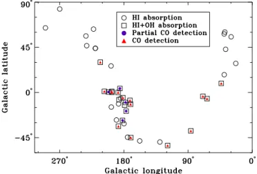
We conducted a follow-up CO survey of 44 of the Millennium sightlines for which OH data were taken. Figure 1 shows the distribution of all observed sources in Galactic coordinates.
The J=1–0 transitions of CO, 13
CO, and C18Owere observed with the Purple Mountain Observatory Delingha (PMODLH) 13.7 m telescope of the Chinese Academy of Sciences. All numbers reported in this section are in units of
Tmb, since the Delingha system automatically corrected for the
main-beam antenna efficiency. The three transitions were observed simultaneously with the 3 mm SIS receiver in 2013 March, 2013 May, 2014 May, and 2016 May. The FFTS wide-band spectral backend has a wide-bandwidth of 1 GHz at a frequency resolution of 61.0 kHz, which corresponds to 0.159 km s−1at
115.0 GHz and 0.166 km s−1at 110.0 GHz. Position-switching
mode was used with reference positions selected from the IRAS Sky Survey Atlas.18The system temperature varied from 210 K to 350 K for CO, and 140 K to 225 K for the13CO and C18O observations. The resulting rms is ∼60 mK for a 0.159 km s−1 channel for 12
CO and ∼30 mK for a 0.166 km s−1
channel for 13CO and C18O, respectively.
The 12CO(J=2–1) data were taken with the Caltech Submillimeter Observatory (CSO) 10.4 m on Maunakea in 2013 July, October, and December. The system temperature varied from 230 to 300 K for12CO(J=2–1), resulting in an rms of ∼35 mK at a velocity resolution of 0.16 km s−1.
To achieve consistent sensitivity among sightlines,
12
CO(J=2–1) spectra toward 3 sources were also obtained with the IRAM 30 m telescope in frequency-switching mode on 2016 May 22 and 23. The integration times of these
observation were between 30 and 90 minutes, resulting in an rms of less than 20 mK at a velocity resolution of 0.25 km s−1.
The astronomical software package Gildas/CLASS19 was used for data reduction, including baseline removal and Gaussian fitting.
3. OH Properties
3.1. Radiative Transfer and Gaussian Analysis
The equations of radiative transfer for ON/OFF source measurements may be written as
TAON( )v h =b (Tex-Tbg-Tc)(1 -e-tv) ( )K , ( )5
TAOFF( )v h =b (Tex-Tbg)(1 -e-tv) ( )K , ( )6 where we assumed a main-beam efficiency ηb=0.5 according
to Heiles et al. (2001)in all subsequent calculations. Texand τv
are the excitation temperature and optical depth of the cold cloud, respectively. TAON( )v and TAOFF( )v are antenna tempera-tures toward and offset from the continuum source, respec-tively. Here, Tc is the compact continuum source brightness
temperature, and Tbgis the background brightness temperature,
consisting of the 2.7 K isotropic CMB and the Galactic synchrotron background at the source position. We adopted the same treatment of the background continuum (Heiles & Troland2003a)
Tbg=2.7+Tbg408(nOH 408 MHz)-2.8, ( )7 where Tbg408 comes from Haslam et al. (1982). The
back-ground continuum contribution from Galactic HIIregions can be safely ignored, since our sources are either at high Galactic latitudes or Galactic Anti-Center longitudes. Typical Tbgvalues
are thus found to be around 3.3 K.
We decomposed the OH spectra into Gaussian components to evaluate the physical properties of OH clouds along the line of sight. Following the methodology of Heiles & Troland (2003a), we assumed a two-phase medium, in which cold gas components are seen in both absorption and emission (i.e., in both the opacity and brightness temperature profiles), while warm gas appears only in emission, i.e., only in brightness temperature (see Heiles & Troland (2003a)for further details). While this technique is generally applicable for both HI and OH, we have only detected OH in absorption in this work. “Warm” OH components in emission have been observed by Liszt & Lucas (1996), although only by the NRAO 43 m and not with the VLA or Nancay in their study. This is consistent with our results in that there is no OH warm enough (> a few hundred K) in our Arecibo beam to be seen in emission, nor do we expect it from astrochemistry considerations.
In brief, the expected profile Texp(v) consists of both
emission and absorption components:
Texp( )v =TB,cold( )v +TB,warm( )v , ( )8 where TB,cold( ) is the brightness temperature of the cold gasv
and TB,warm( ) is the brightness temperature of the the warmv
gas. Both components contribute to the emission profile. The opacity spectrum is obtained by combining the on- and off-source spectra (Equations (5) and (6)), and contains only
Figure 1. Locations of background continuum sources in Galactic coordinates. This plot shows only the 44 sources towards which HIOH and CO were observed. The open circles represent sources with detected HIabsorption only. The squares represent sources with detected HIand OH absorption. The red triangles represent sources with CO detections, in which every detected OH component is also seen in CO. The blue dots represent sources with CO detections, in which some OH components do not have corresponding CO detections. We call these sources “partial CO detections.”
18
http://irsa.ipac.caltech.edu/data/ISSA/ 19http://www.iram.fr/IRAMFR/GILDAS/ 3
cold gas seen in absorption. First, we fit the observed opacity spectrum e− τ( v)with a set of N Gaussian components.
Next, we fit the expected emission profile, Texp, which is
assumed to also consist of the N cold components seen in the absorption spectrum, plus any warm components seen only in emission. We further assume that each component is independent and isothermal with an excitation temperature
Tex,n: v e . 9 n N n v v v 0 1 0, 0,n n 2
å
t = t d = -( ) [( ) ] ( )Here, τ0,n, v0,n, and δvnare respectively the peak optical depth,
central VLSR, and 1/e-width of component n. All the values of
τ0,n, v0,n, and δvn were then obtained through least-squares
fitting. The contribution of the cold components is given by
T v T 1 e e , 10 n N n v v B,cold 0 1 ex, n m n m 0 1
å
= - t åt = -- - = -( ) ( ( )) ( ) ( )where subscript m describes the M absorbing clouds lying in front of the nth cloud. When n=0, the summation over m takes no effect, as there is no foreground cloud.
We obtained the values of excitation temperature Tex,nfrom this fit. As in Heiles & Troland (2003a), we experimented with all possible orders along the line of sight and retained the one that yields the smallest residuals.
In total, we detected 48 OH components toward 21 sightlines. Example spectra and fits are shown in Figures 2
and 3.
3.2. OH Excitation and Optical Depth
Our fitting scheme provides measurements of the excitation conditions and optical depths of the OH gas.
Figure4shows a histogram of optical depths in the two OH main lines, with the 1665 line scaled by a factor of 9/5 (see below). The measured optical depth of both lines peaks at very low values of ∼0.01, with a longer tail extending as high as 0.21 in the 1667 line. As can be seen in Table 2, the uncertainties on these values are generally very small. The OH gas probed by absorption is thus quite optically thin.
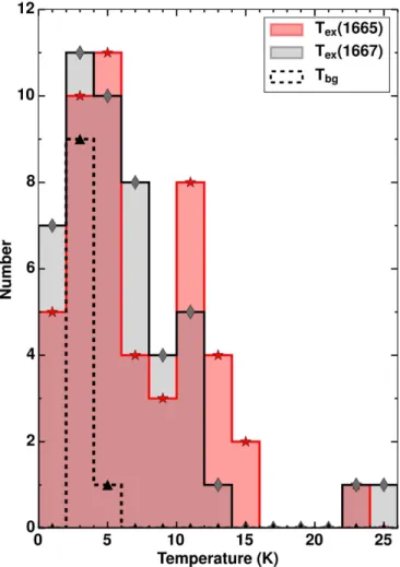
As seen in Figure5, OH excitation temperatures in the two main lines peak at ∼3–4 K and are similar for the two lines. The majority (∼90%) of the components show Tex values
within 2 K of the diffuse continuum background temperature,
Tbg, consistent with measurements from past work (e.g.,
Nguyen-Q-Rieu et al. 1976; Crutcher 1979; Dickey et al.
1981). The probability density distribution (PDF) of the OH excitation temperature can be fitted by a modified normalized lognormal function,20 f T 1 T T 2 exp ln ln 2 . 11 ex ex ex 0 2 2 p s s µ ⎡- -⎣ ⎢ ⎤ ⎦ ⎥ ( ) [ ( ) ( )] ( )
The fit parameters are sensitive to the binning and statistical weighting of the data and are not unique. We chose one solution that preserves the tail of relatively high Tex. The exact
numerical values are less meaningful than the location of the distribution peak and the rough trend of Tex, which are
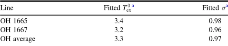
represented in the current fitting. The fit results are shown in Figure 6 and Table 1. The statistical uncertainties are small.
Figure 2. Illustration of derived parameters from the fits to the absorption (upper panel) and expected emission (lower panel) profiles for the source P0428+20. The thin solid lines show the data ; the thick solid lines are the fits. The solid lines below the dashed lines present the residuals for absorption and fitted expected emission, respectively.
Figure 3. Data for the source 3C409. See Figure2for a complete description.
20
Equation (11)differs from the standard lognormal function of x in that it has no variable (x) in the denominator.
4
Similar numerical values are found in fitting both the 1665 and 1667 transitions. A simple average of the two sets of fit parameters is also presented in Table 1. Given the unbiased nature of absorption-selected sightlines and the fact that almost half of the detected OH components lie at low Galactic latitudes ( b∣ ∣ < 5 ), such a generic distribution function may be representative of OH excitation conditions in the Galactic ISM. This tentative conclusion will be refined by future observations. The combined results of Texand τ reflect the complexities in
OH excitation. When the level populations of the OH ground states are in LTE, the excitation temperatures of the 1665 and 1667 MHz lines are equal, and their optical depth ratio (R67/65= τ1667/τ1665) is 1.8. In general, however, we do not
expect OH to be thermally excited. The satellite lines (at 1612 and 1720 MHz) commonly show highly anomalous excitation patterns, with Texthat are strongly subthermal in one line, and
either very high or negative (masing) in the other (e.g., Dawson et al.2014). This may occur due to far-IR or infrared pumping, which can lead to selective overpopulation of either the F=1 or the F=2 level pair (e.g., Guibert et al.1978). The result is that the main line Texmay be very similar, despite the system as
a whole being strongly non-thermally excited.
As shown in Figure 7, most OH components deviate from LTE at more than the formal 1σ uncertainties propagated from the Gaussian fits. The difference between the excitation temperatures, however, mainly falls within 2 K (∣DTex∣<2 K), consistent with values observed in previous absorption measurements toward continuum sources (e.g., Nguyen-Q-Rieu et al.1976; Crutcher1977,1979; Dickey et al.1981).
3.3. OH Column Density
The column densities of the OH components were computed independently from each line according to
N k T A c h dv OH 8 16 5 , 12 1667 ex,1667 1667 2 1667 3 1667
ò
p n t = ( ) ( )Figure 4. Histogram of peak optical depths of the OH Gaussian components. The black bars show the results for the 1667 MHz line and the red bars show 1.8 times the results for the 1665 MHz line.
Figure 5. Histograms of excitation temperature, Tex, of the Gaussian
components for the two OH main lines, and the background continuum temperature Tbg. The number histogram of Tbghas been scaled by a factor of
0.5, for ease of visualization.
Figure 6. Fitting results of the PDFs of OH excitation temperature for both the 1665 and 1667 lines. Fit parameters are given in Table1.
5
N k T A c h dv OH 8 16 3 , 13 1665 ex,1665 1665 2 1665 3 1665
ò
p n t = ( ) ( ) where A1667=7.778×10⁻¹¹ s−1 and A1665=7.177× 10⁻¹¹ s−1are the Einstein A-coefficients of the OH main lines (Destombes et al. 1977). The values are tabulated in Table 2and discussed below.
4. The Relation between HI, CO, and OH
4.1. OH and HI
Regardless of the complexities in the OH excitation, the measured line ratios are generally close to the LTE value of 5/9 with a relatively small scatter. To appropriately utilize both transitions while minimizing the impact of the poorer S/N in the 1665 line, we estimate the total OH column density as
N OH 5N 1665 N 1667
14
9 14
= +
( ) ( ) ( ). The OH column
densi-ties obtained with this method are plotted against the HI
column density of each Gaussian component in Figure 8on a component-by-component basis. Since the HIcomponents are always wider than OH lines, the sum of all OH components was used when multiple OH components coincide with one HI
component.
For non-detections, an upper limit was estimated based on the 1667 MHz spectrum alone, assuming a single Gaussian optical depth spectrum, with a FWHM of 1.0 km/s and peak τ equal to 3 times the spectral rms. For instance, an rms of 1667 MHz absorption spectrum toward 3C138 is 31 mK in brightness temperature. Texwas assumed to be equal to 3.5 K,
the peak of the lognormal function fitted to the Texdistribution
in Figure 6. These values are plotted as triangles in Figure8. Our absorption data set typically has a detection limit around
N(OH);1012cm−2, with a number of higher limits occurring
toward weaker continuum background sources.
Many HIcomponents have no detectable OH. Where OH is detected, there is some suggestion of a weak correlation between the OH and HIcolumn densities. For N(HI)between 1020 and 1021 cm−2 most sources are consistent with an
[OH]/[HI]abundance ratio ∼10−7. 4.2. OH and CO
Both CO and OH are widely used molecular tracers in the ISM. Allen et al. (2012,2015) performed a pilot OH survey toward the Galactic plane around l≈105° and demonstrated the presence of CO-dark molecular gas (DMG): CO emission was absent in more than half of the detected OH spectral features (see also Wannier et al.1993and Barriault et al.2010). Xu & Li (2016)took OH observations across a boundary of the Taurus molecular cloud, revealing that the fraction of DMG decreases from 0.8 in the outer CO poor region to 0.2 in the inner CO abundant region.
Our explicit measurements of CO and OH properties allow us to examine the relation between CO and OH again. Nine OH components are identified as DMG clouds and will be discussed in detail in Section4.3. We focus here on molecular clouds with both OH and CO detections.
CO emission was detected toward 40/49 OH components. CO column density, N(CO), is calculated differently for each of the following three cases:
1. Detection of only12CO(J=1–0).
2. Detection of both12CO(J=1–0) and12CO(J=2–1). 3. Detection of three lines,12CO(J=1–0),12CO(J=2–1),
and13CO(J=1–0) simultaneously.
In LTE, the total column density Ntotof a two-level transition
from upper level u to lower level l is given by
N c A Q g e e d 8 1 , 14 ul u E kT h kT tot 3 3 rot u ex ex
ò
pn t u = -n u ( )where Aulis the spontaneous emission coefficient for transitions
between levels u and l, guis the degeneracy of level u, Euis the
energy of level u, and Texis the excitation temperature. Qrotis
the rotational partition function, given by
Q kT hB hB kT hB kT hB kT 1 3 1 15 4 315 1 315 , 15 rot ex 0 0 ex 0 ex 2 0 ex 3 » + + + + ⎛ ⎝ ⎜ ⎞ ⎠ ⎟ ⎛ ⎝ ⎜ ⎞ ⎠ ⎟ ⎛ ⎝ ⎜ ⎞ ⎠ ⎟ ( )
which is good to <1% when Tex>2 K. B0is the rotational
constant of the molecule.
Table 1
Lognormal Fit Parameters for the OH TexDistribution, as Shown in Figure6
Line Fitted Tex0a Fitted σa
OH 1665 3.4 0.98
OH 1667 3.2 0.96
OH average 3.3 0.97
Note. a
Parameter defined in Equation (11).
Figure 7. Optical depth ratio (R67/65= τ1667/τ1665)as a function of excitation
temperature difference (Tex(1667)−Tex(1665)) for the 1667 and 1665 MHz
OH lines. The horizontal and vertical dashed lines indicate 1.8 and 0.0, the values for LTE excitation. The error bars indicate the 1σ formal uncertainties propagated through from the Gaussian fits. The black points are those consistent with LTE to within the 1σ errors; the red points are inconsistent. The vertical shaded region represents∣DTex∣<2 K.
6
Table 2
Gaussian Fit Parameters for OH main Lines
Source l/b OH(1665) OH(1667)
τ Vlsr ΔV Tex N(OH) τ Vlsr ΔV Tex N(OH) (Name) (°) (km s−1) (km s−1) (K ) (1014 cm−2) (km s−1) (km s−1) (K ) (1014 cm−2) 3C105 187.6/−33.6 0.0158±0.0003 8.14±0.01 0.97±0.02 4.93±0.5 0.32±0.26 0.0268±0.0003 8.17±0.0 0.96±0.01 3.96±0.34 0.24±0.13 3C105 187.6/−33.6 0.0062±0.0003 10.23±0.02 1.03±0.05 8.49±1.26 0.23±0.44 0.0107±0.0003 10.26±0.01 1.03±0.03 7.64±0.88 0.2±0.22 3C109 181.8/−27.8 0.0022±0.0003 9.16±0.1 1.0±0.24 23.68±3.66 0.22±0.73 0.0036±0.0004 9.22±0.07 1.02±0.17 24.13±2.5 0.21±0.36 3C109 181.8/−27.8 0.0035±0.0003 10.44±0.06 0.95±0.15 14.76±2.33 0.21±0.56 0.0057±0.0004 10.58±0.05 1.04±0.11 13.92±1.58 0.19±0.29 3C123 170.6/−11.7 0.0191±0.0008 3.65±0.06 1.19±0.11 11.08±1.79 1.08±1.26 0.0347±0.0012 3.71±0.06 1.22±0.1 11.2±1.26 1.13±0.69 3C123 170.6/−11.7 0.0431±0.0023 4.43±0.01 0.53±0.03 6.42±1.22 0.62±0.57 0.0919±0.004 4.46±0.01 0.53±0.02 7.31±0.75 0.84±0.29 3C123 170.6/−11.7 0.0338±0.0008 5.37±0.01 0.92±0.04 11.62±1.11 1.53±0.8 0.0784±0.0012 5.47±0.01 0.92±0.02 8.13±0.61 1.38±0.37 3C131 171.4/−7.8 0.0065±0.0005 4.55±0.02 0.56±0.06 12.67±1.53 0.2±0.3 0.0103±0.0006 4.56±0.02 0.62±0.05 7.51±1.04 0.11±0.16 3C131 171.4/−7.8 0.0074±0.0006 6.8±0.06 2.97±0.2 10.46±0.86 0.98±0.94 0.0111±0.0005 6.68±0.05 3.32±0.15 11.08±0.59 0.96±0.49 3C131 171.4/−7.8 0.0167±0.0007 6.59±0.01 0.42±0.02 2.66±0.84 0.08±0.19 0.0259±0.0008 6.58±0.01 0.43±0.02 4.15±0.58 0.11±0.1 3C131 171.4/−7.8 0.0521±0.0007 7.23±0.0 0.55±0.01 5.03±0.25 0.62±0.13 0.0858±0.0007 7.23±0.0 0.59±0.01 5.43±0.16 0.65±0.07 3C132 178.9/−12.5 0.0033±0.0002 7.82±0.03 0.89±0.08 15.72±2.08 0.19±0.45 0.0056±0.0003 7.79±0.02 0.81±0.05 23.1±1.27 0.25±0.18 3C133 177.7/−9.9 0.1009±0.001 7.66±0.0 0.53±0.0 2.97±0.22 0.68±0.16 0.2132±0.0016 7.68±0.0 0.52±0.0 1.33±1.24 0.35±0.7 3C133 177.7/−9.9 0.0148±0.001 7.94±0.02 1.23±0.03 5.9±3.41 0.46±2.18 0.0333±0.0015 7.96±0.02 1.23±0.02 6.11±2.22 0.59±1.18 3C154 185.6/4.0 0.0266±0.0006 −2.32±0.01 0.74±0.03 2.61±0.57 0.22±0.3 0.0428±0.0007 −2.34±0.01 0.71±0.02 2.69±0.35 0.19±0.12 3C154 185.6/4.0 0.01±0.0005 −1.39±0.04 0.83±0.09 6.15±1.43 0.22±0.51 0.0179±0.0006 −1.34±0.03 0.91±0.06 4.7±0.74 0.18±0.21 3C154 185.6/4.0 0.0038±0.0004 2.23±0.06 1.12±0.16 6.62±3.22 0.12±0.95 0.0054±0.0005 2.18±0.06 1.33±0.14 2.1±1.99 0.04±0.46 3C167 207.3/1.2 0.0109±0.0019 18.53±0.11 1.27±0.26 4.87±2.23 0.29±1.26 0.0108±0.0013 17.66±0.16 2.71±0.4 4.65±1.49 0.32±1.0 3C18 118.6/−52.7 0.003±0.0003 −8.53±0.11 2.5±0.19 10.93±1.99 0.35±1.16 0.006±0.0003 −8.33±0.05 2.5±0.1 9.27±0.86 0.33±0.39 3C18 118.6/−52.7 0.0056±0.0004 −7.82±0.02 0.68±0.06 2.05±2.03 0.03±0.44 0.0078±0.0005 −7.85±0.01 0.6±0.04 1.0±0.0 0.01±0.0 3C207 213.0/30.1 0.0152±0.0002 4.55±0.01 0.77±0.01 3.17±0.42 0.16±0.17 0.0268±0.0002 4.55±0.0 0.78±0.01 2.57±0.2 0.13±0.06 3C409 63.4/−6.1 0.0062±0.0007 14.63±0.14 1.86±0.15 11.37±1.9 0.55±1.19 0.0057±0.0008 14.7±0.18 1.68±0.18 7.8±3.86 0.18±1.15 3C409 63.4/−6.1 0.0199±0.0012 15.4±0.01 0.89±0.04 0.17±0.86 0.01±0.46 0.0273±0.0016 15.41±0.01 0.86±0.03 0.2±0.0 0.01±0.0 3C410 69.2/−3.8 0.0121±0.0003 6.25±0.01 1.03±0.03 9.4±0.97 0.5±0.47 0.025±0.0004 6.29±0.01 1.19±0.02 4.31±0.43 0.3±0.19 3C410 69.2/−3.8 0.0043±0.0003 10.7±0.04 0.7±0.09 11.26±3.32 0.14±0.65 0.0084±0.0005 10.72±0.04 0.8±0.09 4.42±1.55 0.07±0.27 3C410 69.2/−3.8 0.0053±0.0003 11.67±0.04 0.84±0.09 5.74±2.44 0.11±0.64 0.0114±0.0005 11.68±0.03 0.81±0.07 2.92±1.14 0.06±0.23 3C454.3 86.1/−38.2 0.0023±0.0001 −9.67±0.03 1.63±0.07 4.61±2.14 0.07±0.72 0.0044±0.0001 −9.55±0.02 1.37±0.04 8.25±1.22 0.12±0.26 3C75 170.3/−44.9 0.0072±0.0003 −10.36±0.03 1.32±0.07 3.64±1.09 0.15±0.52 0.0142±0.0003 −10.36±0.02 1.25±0.04 3.91±0.6 0.16±0.21 4C13.67 43.5/9.2 0.0474±0.0037 4.88±0.05 1.3±0.12 10.43±0.9 2.73±1.13 0.057±0.004 4.95±0.05 1.46±0.12 10.37±0.62 2.04±0.56 4C22.12 188.1/0.0 0.0059±0.0009 −2.84±0.06 0.79±0.17 6.91±2.35 0.14±0.61 0.0103±0.001 −2.73±0.04 0.8±0.11 6.75±1.28 0.13±0.25 4C22.12 188.1/0.0 0.0172±0.0011 −1.78±0.02 0.56±0.05 4.67±0.95 0.19±0.3 0.0356±0.0012 −1.78±0.01 0.54±0.02 3.8±0.46 0.17±0.11 G196.6+0.2 196.6/0.2 0.0043±0.0005 3.22±0.1 1.67±0.25 10.95±2.34 0.34±1.1 0.0065±0.0005 3.43±0.09 2.5±0.24 8.85±1.24 0.34±0.59 G197.0+1.1 197.0/1.1 0.0124±0.0005 4.83±0.03 1.84±0.09 5.2±0.65 0.5±0.57 0.0188±0.0007 4.72±0.03 1.59±0.07 5.51±0.5 0.39±0.26 G197.0+1.1 197.0/1.1 0.0057±0.0008 7.46±0.04 0.61±0.1 1.0±0.0 0.01±0.0 0.0075±0.0011 7.34±0.04 0.6±0.1 1.0±0.0 0.01±0.0 G197.0+1.1 197.0/1.1 0.0053±0.0006 16.41±0.09 1.17±0.22 8.76±1.91 0.23±0.69 0.0094±0.0017 16.34±0.12 0.95±0.19 7.07±1.33 0.15±0.29 G197.0+1.1 197.0/1.1 0.0069±0.0008 17.65±0.05 0.71±0.12 5.35±1.88 0.11±0.47 0.0124±0.001 17.45±0.12 1.22±0.21 7.15±0.89 0.26±0.29 G197.0+1.1 197.0/1.1 0.0237±0.0009 32.01±0.01 0.56±0.02 3.41±0.62 0.19±0.23 0.0428±0.0012 32.01±0.01 0.53±0.02 4.35±0.39 0.23±0.1 P0428+20 176.8/−18.6 0.0015±0.0002 3.6±0.08 1.06±0.2 13.3±4.09 0.09±0.71 0.0029±0.0003 3.55±0.04 0.75±0.09 4.56±2.56 0.02±0.25 P0428+20 176.8/−18.6 0.0076±0.0002 10.7±0.02 1.1±0.04 13.29±0.79 0.47±0.32 0.0137±0.0003 10.7±0.01 1.11±0.02 11.71±0.45 0.42±0.14 P0531+19 186.8/−7.1 0.0011±0.00024 1.559±0.087 0.814±0.214 3.49±4.37 0.0133±0.0169 0.00089±0.00024 1.85±0.139 1.053±0.346 4.01±7.1 0.0089±0.0162 T0526+24 181.4/−5.2 0.0158±0.0058 7.58±0.29 1.66±0.74 13.57±2.78 1.51±2.61 0.0359±0.0059 7.49±0.15 1.97±0.39 10.21±1.2 1.7±1.15 T0629+10 201.5/0.5 0.004±0.0026 0.16±0.19 0.64±0.49 4.07±2.23 0.05±0.39 0.0113±0.0023 0.33±0.22 0.97±0.43 3.22±0.96 0.08±0.24 T0629+10 201.5/0.5 0.0378±0.0129 3.13±0.28 0.99±0.43 0.59±0.66 0.09±0.54 0.0769±0.0046 4.17±0.06 3.17±0.22 0.92±1.87 0.53±3.88 T0629+10 201.5/0.5 0.0168±0.0016 1.47±0.11 1.43±0.44 1.49±0.46 0.15±0.37 0.0206±0.0034 1.3±0.1 0.8±0.2 0.5±0.0 0.02±0.01 7 The Astrophysical Journal Supplement Series, 235:1 (15pp ), 2018 March Li et al.
Table 2 (Continued)
Source l/b OH(1665) OH(1667)
τ Vlsr ΔV Tex N(OH) τ Vlsr ΔV Tex N(OH) (Name) (°) (km s−1) (km s−1) (K ) (1014 cm−2) (km s−1) (km s−1) (K ) (1014 cm−2) T0629+10 201.5/0.5 0.163±0.0281 3.61±0.02 0.61±0.04 2.33±0.13 0.98±0.22 0.2147±0.0045 3.55±0.0 0.6±0.02 3.1±0.13 0.95±0.09 T0629+10 201.5/0.5 0.0812±0.002 4.62±0.01 0.78±0.03 1.23±0.29 0.33±0.27 0.1004±0.0044 4.64±0.01 0.36±0.02 1.48±0.26 0.13±0.07 T0629+10 201.5/0.5 0.075±0.0018 6.09±0.02 1.05±0.05 3.74±0.2 1.25±0.25 0.1011±0.0043 6.1±0.01 0.64±0.04 4.46±0.25 0.69±0.13 T0629+10 201.5/0.5 0.0371±0.0031 6.99±0.02 0.49±0.06 4.28±0.29 0.33±0.13 0.0744±0.0036 6.93±0.02 0.64±0.05 3.99±0.22 0.45±0.1 T0629+10 201.5/0.5 0.0174±0.0018 7.9±0.05 0.83±0.13 3.54±0.46 0.22±0.22 0.0295±0.0025 7.95±0.03 0.71±0.08 3.46±0.42 0.17±0.12 8 The Astrophysical Journal Supplement Series, 235:1 (15pp ), 2018 March Li et al.
τνis the optical depth of the line, and is related to brightness
temperature, Tb, through the radiative transfer equation J T( )b =f J T[ ( ex)-J T( bg)][1-e-tv], (16) where f is the beam filling factor and J T( )=
hn k ehn kT -1
( ) ( ).
When only 12CO(J=1–0) is detected (case 1), we do not adopt the optically thick assumption but adopt the assumption that the excitation temperature of12CO is 10 K as suggested by Goldsmith et al. (2008)in the Taurus cloud. Optical depth τv
can be derived from Equation (16). Then the total column density of 12CO can be derived through the combination of Equations (14)and (15).
For case 2, we adopted the assumption of optically thin
12CO(J=1–0) and 12CO(J=2–1) lines. This is reasonable
since there is no 13CO(J=1–0) detection and the corrected antenna temperatures of CO are smaller than 1 K (see, e.g., source 3C105 in Figure 13). The excitation temperature of
12
CO, Tex, is then obtained from the following equation
e e e A g A g e e T d T d 1 2 1 1 , 17 T T T T T T T 11.06 16.59 5.53 5.53 5.53 21 3 10 1 10 3 21 2 11.06 5.53 R21 R10 bg ex ex bg ex bg bg
ò
ò
n n u u -- = ´ -- -⎡ ⎣ ⎢ ⎤ ⎦ ⎥ ( )where TR=J(Tb). Once Texin Equation (17) is determined, N(12CO) is derived as done in case 1.
When both12CO(J=1–0) and13CO(J=1–0) are detected as in case 3, we assume τ10(12CO)?1 and derive Texand
τ10(13CO) via: T T 5.53 ln 1 5.532 CO 0.819 . 18 ex R12 1 = + + -⎧ ⎨ ⎩ ⎡ ⎣ ⎢ ⎤ ⎦ ⎥⎫⎬ ⎭ ( ) ( ) T e CO ln 1 CO 5.29 1 0.16 . 19 T 1013 R 13 5.29 1 1 ex t = - - -⎧ ⎨ ⎩ ( ) ( )([ ] ) } ( )
Ntot(13CO) is then obtained using Equation (15), from which
we compute Ntot(12CO) by assuming [12C]/[13C]=68 (Milam
et al.2005).
The central velocities of derived OH components are used as initial estimates for CO fitting with the CLASS/GILDAS software. The properties of the fitted CO components are shown in Table 3, and the above calculations of CO excitation temperature and total column density are based on the derived Gaussian fitting results. The coincidence between OH and CO components is judged by central velocity. The velocity difference should be less than 0.5 km s−1. We plot the relation between OH and CO column density
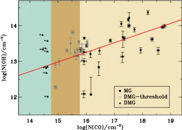
in Figure9. A positive correlation between log(N(OH)) and log(N(CO)) is seen. Least-squares fitting yields the relation log N OH( ( ))=8.160.8980.898+0.3160.0540.054log N CO( ( )). The linear Pearson correlation coefficient is 0.69, indicating a strong correlation. This result is consistent with Allen et al. (2015), where an apparent correlation was found between strong12CO
emission and OH emission.
4.3. CO-dark Molecular Gas
All-sky CFA CO survey data (Dame et al.2001)have been widely used to investigate the distribution of CO on large scales. Planck Collaboration et al. (2011), for example, analyzed Planck data along with the CFA CO survey to probe the large-scale DMG distribution. In principle, the definition of a DMG cloud depends on the sensitivity of the CO data employed. For example, Donate & Magnani (2017)found that the fraction of CO-dark molecular gas relative to total H2
decreased from 58% to 30% in the Pegasus-Pisces region when higher sensitivity CO data were taken. In this study, the representative 1σ sensitivity of CFA CO data is about σCFA=0.25 K per 0.65 km s−1. Using this as an illustrative
detection threshold, we here identify components as “DMG-threshold clouds” in cases where CO emission would be undetected at 3σCFAbut is detected at the higher sensitivity of
the present work.
We compare the Gaussian components seen in HI absorp-tion, OH absorpabsorp-tion, and CO emission. A total of 219 HIand 49 OH absorption components were detected. Most OH components can be associated with an HI component within a velocity offset of 1.0 km s−1, except for three sources with
offsets of about 1.5 km s−1. There are four general categories of
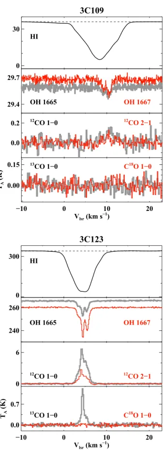
clouds, three of which are illustrated in Figure 10. Toward 3C192, only HI is present, typical of CNM. Toward 3C133, HI, OH, and several CO and CO isotopologues are all detected, which is representative of “normal” molecular clouds. Toward 3C132, there exists a component with HIand OH absorption, but no CO emission, representing DMG. An example of a DMG-threshold cloud can be found in the spectra of 3C109 (Figure13), where only weak ( 0.1 K) CO is detected. In our sample, there are 77.6% CNM, 4.1% DMG, 6.9% DMG-threshold, and 11.4% molecular clouds. In terms of
Figure 8. OH column densities derived from the 1667 line, N(OH), vs. HI column densities, N(HI), both on a Gaussian component-by-component basis. The triangles depict approximate upper limits for HIcomponents where OH was not detected (see Section4.1).
9
Table 3
Gaussian Fit Parameters of CO Data
Source l/b 12CO(1–0) 12CO(2–1) 13CO(1–0) Ob N(12CO)
Tpeak a Vlsr ΔV Tpeak a Vlsr ΔV Tpeak a Vlsr ΔV (Name) (°) K (km s−1) (km s−1) K (km s−1) (km s−1) K (km s−1) (km s−1) (1017 )cm−2 3C105 187.6/−33.6 1.0 8.07±0.03 0.77±0.06 0.3 8.05±0.03 0.45±0.06 K K K 0 0.1032±0.0083 3C105 187.6/−33.6 0.9 10.81±0.03 0.68±0.09 0.3 10.20±0.03 0.74±0.08 K K K 1 0.0651±0.0082 3C109 181.8/−27.8 K K K K K K K K K 0 K 3C109 181.8/−27.8 0.1 10.69±0.15 1.52±0.42 K K K K K K 1 0.0206±0.0057 3C123 170.6/−11.7 2.8 3.99±0.00 1.87±0.03 1.4 3.75±0.03 1.71±0.10 0.1 3.87±0.23 1.33±0.38 0 1.7736±0.0312 3C123 170.6/−11.7 3.2 4.18±0.00 0.47±0.01 2.2 4.07±0.01 0.51±0.03 1.1 4.41±0.01 0.48±0.02 1 5.1962±0.1415 3C123 170.6/−11.7 3.2 5.21±0.01 1.62±0.02 1.8 5.14±0.03 1.43±0.07 0.3 5.17±0.06 0.93±0.14 2 3.1336±0.0483 3C131 171.4/−7.8 0.7 4.59±0.16 0.71±0.16 0.4 4.56±0.05 0.84±0.13 K K K 0 0.0506±0.0113 3C131 171.4/−7.8 1.8 6.88±0.16 2.07±0.16 0.9 6.92±0.01 1.64±0.10 0.2 6.81±0.05 0.96±0.12 1 3.2982±0.3194 3C131 171.4/−7.8 1.2 6.64±0.16 0.72±0.16 0.8 6.64±0.03 0.67±0.06 K K K 2 0.0842±0.0187 3C131 171.4/−7.8 0.7 7.18±0.16 0.48±0.16 0.3 7.10±0.04 0.41±0.01 K K K 3 0.0335±0.0112 3C132 178.9/−12.5 K K K K K K K K K 0 K 3C133 177.7/−9.9 3.1 7.43±0.00 0.86±0.01 2.0 7.50±0.01 0.81±0.02 0.3 7.36±0.03 0.70±0.06 0 2.0087±0.0248 3C133 177.7/−9.9 K K K K K K K K K 1 K 3C154 185.6/4.0 3.7 −2.41±0.01 1.23±0.02 2.1 −2.37±0.35 1.24±0.35 0.9 −2.06±0.01 1.13±0.03 0 8.6360±0.1185 3C154 185.6/4.0 3.0 −1.62±0.01 0.94±0.01 1.5 −1.57±0.35 0.79±0.35 K K K 1 0.2972±0.0047 3C154 185.6/4.0 K K K K K K K K K 2 K 3C167 207.3/1.2 0.7 17.47±0.31 1.59±0.57 0.3 17.64±0.25 1.62±0.32 K K K 0 0.1098±0.0394 3C18 118.6/−52.7 0.5 −8.22±0.06 1.31±0.14 0.1 −8.32±0.14 0.56±0.32 K K K 0 0.1078±0.0117 3C18 118.6/−52.7 0.2 −7.10±0.08 0.40±0.15 0.1 −7.74±0.17 0.33±0.30 K K K 1 0.0082±0.0030 3C207 213.0/30.1 0.4 4.79±0.02 1.00±0.04 0.2 4.74±0.09 0.80±0.19 K K K 0 0.0443±0.0019 3C409 63.4/−6.1 0.2 13.82±0.30 1.25±0.44 0.2 14.44±0.24 2.08±0.23 K K K 0 0.0281±0.0099 3C409 63.4/−6.1 1.3 15.20±0.04 1.13±0.08 0.6 15.23±0.01 1.02±0.05 K K K 1 0.1479±0.0105 3C410 69.2/−3.8 1.4 5.96±0.01 0.81±0.04 1.1 5.92±0.01 0.52±0.03 0.1 5.74±0.06 0.73±0.26 0 0.7262±0.0545 3C410 69.2/−3.8 0.2 10.97±0.27 0.45±0.64 K K K K K K 1 0.0154±0.0219 3C410 69.2/−3.8 0.2 11.54±0.40 0.44±0.50 K K K K K K 2 0.0168±0.0192 3C454.3 86.1/−38.2 0.9 −9.41±0.03 0.79±0.07 0.2 −9.62±0.05 1.20±0.14 K K K 0 0.0713±0.0063 3C75 170.3/−44.9 1.6 −10.28±0.01 0.90±0.03 1.1 −10.29±0.02 0.62±0.05 K K K 0 0.1420±0.0042 4C13.67 43.5/9.2 6.6 4.75±0.01 1.54±0.02 3.5 4.89±0.01 1.65±0.02 1.2 4.91±0.01 0.99±0.03 0 15.6457±0.1521 4C22.12 188.1/0.0 1.6 −2.58±0.16 0.94±0.16 1.0 −2.44±0.01 1.19±0.03 0.2 −2.47±0.12 0.82±0.21 0 1.9370±0.2582 4C22.12 188.1/0.0 1.3 −1.96±0.16 0.67±0.16 K K K K K K 1 0.1639±0.0387 G196.6+0.2 196.6/0.2 0.3 3.42±0.14 2.14±0.25 K K K K K K 0 0.0575±0.0067 G197.0+1.1 197.0/1.1 2.9 5.07±0.16 1.93±0.16 1.4 4.92±0.03 1.90±0.05 0.2 5.04±0.10 1.39±0.24 0 2.2626±0.1892 G197.0+1.1 197.0/1.1 0.8 7.18±0.16 1.01±0.16 0.6 7.33±0.04 1.20±0.08 K K K 1 0.0825±0.0130 G197.0+1.1 197.0/1.1 0.4 16.34±0.16 0.97±0.16 0.0 16.63±0.35 2.60±0.35 K K K 2 0.0395±0.0065 G197.0+1.1 197.0/1.1 0.4 17.39±0.16 1.18±0.16 0.1 17.52±0.35 1.86±0.35 K K K 3 0.0489±0.0066 G197.0+1.1 197.0/1.1 0.5 32.24±0.05 1.24±0.02 0.3 32.28±0.35 0.76±0.35 K K K 4 0.0704±0.0010 P0428+20 176.8/−18.6 K K K K K K K K K 0 K P0428+20 176.8/−18.6 0.9 10.71±0.02 0.89±0.05 0.3 10.59±0.06 0.98±0.14 K K K 1 0.0857±0.0049 T0526+24 181.4/−5.2 8.0 6.86±0.00 1.07±0.01 6.3 6.90±0.00 0.89±0.01 0.5 6.95±0.02 0.83±0.04 0 3.3663±0.0226 T0629+10 201.5/0.5 K K K K K K K K K 0 K T0629+10 201.5/0.5 K K K K K K K K K 1 K T0629+10 201.5/0.5 1.2 1.13±0.16 2.20±0.16 0.5 1.30±0.16 2.24±0.16 K K K 2 0.2812±0.0203 T0629+10 201.5/0.5 5.5 2.85±0.16 1.25±0.16 5.0 2.74±0.16 1.15±0.16 4.1 3.71±0.17 1.64±0.17 3 59.8330±8.2582 10 The Astrophysical Journal Supplement Series, 235:1 (15pp ), 2018 March Li et al.
Table 3 (Continued)
Source l/b 12CO(1–0) 12CO(2–1) 13CO(1–0) Ob N(12CO)
Tpeak a Vlsr ΔV Tpeak a Vlsr ΔV Tpeak a Vlsr ΔV (Name) (°) K (km s−1) (km s−1) K (km s−1) (km s−1) K (km s−1) (km s−1) (1017 )cm−2 T0629+10 201.5/0.5 8.3 4.49±0.16 1.85±0.16 7.4 4.58±0.16 1.63±0.16 2.5 4.99±0.17 1.06±0.17 4 36.1908±3.5195 T0629+10 201.5/0.5 6.6 6.19±0.16 1.40±0.16 6.1 6.36±0.16 1.33±0.16 3.7 6.01±0.17 0.74±0.17 5 51.6879±6.1885 T0629+10 201.5/0.5 1.9 7.16±0.16 1.57±0.16 1.4 7.28±0.16 1.39±0.16 1.2 6.66±0.17 0.75±0.17 6 21.8699±2.4927 T0629+10 201.5/0.5 K K K K K K K K K 7 K Notes. a
Tpeak: Peak brightness temperature corrected for main-beam efficiency of the telescope.
b
O: Order of the cold components along the line of sight, beginning with 0; larger numbers mean larger distances along the line of sight.
11 The Astrophysical Journal Supplement Series, 235:1 (15pp ), 2018 March Li et al.
detectability in absorption, the apparent DMG clouds (DMG and DMG-threshold) are similar to molecular clouds with CO emission.
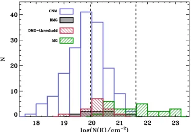
The statistics of hydrogen column density are presented in Figure11. The hydrogen column density of DMG clouds (DMG and DMG-threshold) falls between N(H) ∼1020cm−2and 4×
1021cm−2, corresponding to a extinction range A
V∼0.05 to
2 mag. Within this “intermediate” extinction range, the self-shielding of H2is complete, while that of CO is not. All N(H) in
this work refer to hydrogen column density based on HI
absorption and CO emission measurements. Comparison with
N(H2) based on Planck results will be published in a separate
paper (Hiep et al. in prep). The abundance of measured CO is thus expected to be less than the canonical value of 10−4and to
vary with extinction. Our detection statistics of OH in DMGs are consistent with a picture in which gas in this intermediate extinction range is still evolving chemically. OH is thus a potentially good tracer of diffuse gas with intermediate extinction, namely between the self-shielding thresholds of H2and CO. Such a suggestion has been borne out by detailed
studies of individual regions with more complete information. Xu & Li (2016), for example, found much tighter X-factors in both OH and CH than in CO, for gases in the intermediate extinction region of the Taurus molecular cloud.
5. Implications of the Absorption Survey
The expected locations and abundance of OH should make it an excellent tracer of DMG. However, due both to low optical depths and low contrast between the main line excitation temperatures and the Galactic diffuse continuum background, OH is generally difficult to detect in emission. Large-scale mapping of OH therefore requires extremely high sensitivity observations and/or the existence of a bright continuum background against which the lines may be seen in absorption. A handful of studies have accomplished the former over very
limited regions in the Northern Hemisphere local ISM (Barriault et al. 2010; Allen et al. 2012, 2015; Cotten et al. 2012). The SPLASH project (Dawson et al. 2014) has greatly improved on the sensitivities of previous large-scale surveys in the south, to map OH (primarily in absorption) over >150 square degrees of the bright inner Galaxy. However, for outer-Galaxy and off-plane regions, the most practical approach will make use of upcoming radio telescopes to conduct comprehensive absorption surveys, of the kind piloted here.
The Five-hundred-meter Aperture Spherical radio Telescope (FAST) commenced observing in 2016 September. The unprecedented sensitivity of FAST and its early science instruments (Li et al.2013)should make feasible an HI+OH absorption survey, in the mode of the Millennium Survey, but with 10 times more sources. Figure12shows the distribution of potential continuum sources available to FAST. In the coming decades, the SKA1 will provide the survey speed and sensitivity to measure absorption with a source density of between a few to a few tens per square degree (McClure-Griffiths et al. 2015). This makes feasible an all-sky “absorption-image,” mapping out a fine grid of ISM excitation temperature and column density over a very large fraction of the sky. Based on similar excitation and sensitivity considera-tions, ALMA is a powerful instrument for obtaining systematic and sensitive absorption measurements of millimeter lines in diffuse gas. CO and HCO+in diffuse gas, in particular, will be much better constrained in terms of excitation temperature and column densities through ALMA absorption observations than through emission measurements. Combining both radio and millimeter absorption surveys in the coming decade, we will quantify the DMG and provide definitive answers to questions like the global star formation efficiency.
6. Conclusions
Utilizing unpublished OH absorption measurements from the Millennium Survey and our own follow-up CO surveys, we carried out an analysis of the excitation conditions and quantity of OH along 44 sightlines through the Local ISM and Galactic Plane. CO was observed toward these positions. 49 OH components were detected toward 22 of these sightlines. The conclusions are as follows:
1. The excitation temperature of OH peaks around 3.4 K and follows a modified normalized lognormal distribution,
f T 1 T 2 exp ln ln 3.4 K 2 . ex ex 2 2 p s s µ ⎡- -⎣ ⎢ ⎤ ⎦ ⎥ ( ) [ ( ) ( )]
The majority of OH gas in our sample, presumably representative of the Milky Way, thus has an excitation temperature close to the background (CMB plus synchrotron), providing an explanation of why OH has historically been so difficult to detect in emission. 2. The OH main lines are generally not in LTE, with a
moderate excitation temperature difference of T∣ ex(1667)
-Tex(1665)∣<2 K.
3. The OH emission is optically thin; the distribution of τ1667 peaks at ∼0.01, with the highest value in our
sample being equal to 0.22.
4. A weak correlation between N(OH) and N(HI)was found. The abundance ratio [OH]/[HI]has a median of 10−7. Figure 9. CO column densities, N(CO), vs. OH column densities, N(OH) for
three categories of clouds. Molecular clouds (MG) with CO detections are represented with black filled circles in the light yellow region. DMG-threshold clouds are represented by gray filled circles in the dark yellow region. In these clouds, CO emission is detected at the CO sensitivity of this work but would be detected at less than 3σ under a CO sensitivity of 0.25 K per 0.65 km s−1,
typical of the CFA CO survey (Dame et al.2001). The black triangles in the blue region represent DMG clouds in which CO emission is not detected at the CO sensitivity of the present work. The red solid line represents the least-squares fit result to the MG and DMG-threshold clouds.
12
5. N(OH) and N(CO) are linearly correlated when both are detected, which is consistent with previous observations. 6. Whether a cloud is designated as DMG depends on the sensitivity of the CO data. By comparing with the CfA CO survey data of Dame et al. (2001) we find that the fraction of DMG components would increase by a factor of ∼2.5 compared to our results, had this less sensitive data set been used. To highlight this difference, we designated clouds that would be “CO-dark” in the CfA survey as “DMG-threshold” clouds in this work. 7. About 49% of all detected OH absorption clouds are
CO-dark, namely, either DMG or DMG-threshold. The absence of CO emission toward these OH components implies that OH serves as a more effective tracer than
CO of diffuse molecular gas within AV∼0.05 to
2 mag.
8. Given the low opacity and the low excitation temperature of the Galactic OH gas, sensitive absorption surveys made feasible by upcoming large telescopes, such as FAST and SKA, are needed for a comprehensive inventory of Galactic cold gas.
This work is supported by the National Key R&D Program of China 2017YFA0402600 and International
Figure 10. Representative spectra as described in Section4.3. The 3C192 sightline has only HIseen in absorption. One component of the 3C133 sightline has OH and HIin absorption and CO and its isotopologues in emission. The 3C132 sightline has one gas component with both OH and HI, but no detectable CO transitions.
Figure 11. Histogram of hydrogen column density, N(H), for CNM (blue), DMG (filled gray), the DMG-threshold (red), and the molecular cloud (MG, green). N(H) contains contributions from HIfor CNM, DMG, and the DMG-threshold cloud. Both HI and H2 (transforming from CO measurements,
N(H2)=N(CO)/1×10−4)are included for the MG cloud. The left and right
dashed lines represent N(H)=9.4×1019 cm−2 (visual extinction A
V=
0.05 mag) and 3.8×10²¹
cm−2(A
V= 2 mag), respectively.
Figure 12. Distribution of continuum point sources within the area of FAST sky coverage (limits shown with orange), which covers a declination range of −14°.35 to 65°.65. The red circles represent 372 sources with flux densities greater than 2.5 Jy in the NVSS survey. In initial observation periods, FAST will adopt a drift scan mode. The threshold of 2.5 Jy corresponds to a 3σ detection in OH absorption for gas with an optical depth of 0.01, in a drift scan of 12 s, at a velocity resolution of 0.25 km s−1, with a system temperature of
25 K. The blue filled circles represent 1071 sources with flux densities greater than 1.25 Jy in the NVSS survey. The threshold of 1.25 Jy allows for a 3σ detection for OH having an optical depth of 5.5×10⁻³in a total observing
time of 10 minutes (ON+OFF) in tracking mode. The gray background is the integrated HI intensity map from the LAB HI survey (Hartmann & Burton1997; Arnal et al.2000; Bajaja et al.2005). The limits of the coverage of Arecibo are shown with green solid lines. The positions of the 44 point sources used in this paper are plotted with yellow filled squares.
13
Partnership Program of Chinese Academy of Sciences No. 114A11KYSB20160008. D.L. acknowledges support from the “CAS Interdisciplinary Innovation Team” program. J.R.D. is
the recipient of an Australian Research Council DECRA Fellowship (project number DE170101086). This work was carried out in part at the Jet Propulsion Laboratory, which is
Figure 13. Reference spectra of HI, OH, and CO toward continuum sources. (The complete figure set (11 images) is available.)
14
operated for NASA by the California Institute of Technology. L.B. acknowledges support from CONICYT Project PFB06. CO data were observed with the Delingha 13.7 m telescope of the Qinghai Station of Purple Mountain Observatory (PMODLH), the Caltech Submillimeter Observatory (CSO), and the IRAM 30 m telescope. The authors appreciate all the staff members of the PMODLH, CSO, and the IRAM 30 m Observatory for their help during the observations. We thank Lei Qian and Lei Zhu for their help in CSO observations.
ORCID iDs
Di Li https://orcid.org/0000-0003-3010-7661
Ningyu Tang https://orcid.org/0000-0002-2169-0472
J. R. Dawson https://orcid.org/0000-0003-0235-3347
Paul F. Goldsmith https://orcid.org/0000-0002-6622-8396
Steven J. Gibson https://orcid.org/0000-0002-1495-760X
Claire E. Murray https://orcid.org/0000-0002-7743-8129
N. M. McClure-Griffiths https://orcid.org/0000-0003-2730-957X
John Dickey https://orcid.org/0000-0002-6300-7459
Jorge Pineda https://orcid.org/0000-0001-8898-2800
L. Bronfman https://orcid.org/0000-0002-9574-8454
References
Allen, R. J., Hogg, D. E., & Engelke, P. D. 2015,AJ,149, 123
Allen, R. J., Ivette Rodríguez, M., Black, J. H., & Booth, R. S. 2012, AJ,
143, 97
Arnal, E. M., Bajaja, E., Larrarte, J. J., Morras, R., & Pöppel, W. G. L. 2000, A&AS,142, 35
Bajaja, E., Arnal, E. M., Larrarte, J. J., et al. 2005,A&A,440, 767
Barriault, L., Joncas, G., Lockman, F. J., & Martin, P. G. 2010, MNRAS,
407, 2645
Bihr, S., Beuther, H., Ott, J., et al. 2015,A&A,580, A112
Boyce, P. J., & Cohen, R. J. 1994, A&AS,107, 563
Caswell, J. L., & Haynes, R. F. 1975,MNRAS,173, 649
Colgan, S. W. J., Salpeter, E. E., & Terzian, Y. 1989,ApJ,336, 231
Cotten, D. L., Magnani, L., Wennerstrom, E. A., Douglas, K. A., & Onello, J. S. 2012,AJ,144, 163
Crutcher, R. M. 1977,ApJ,216, 308
Crutcher, R. M. 1979,ApJ,234, 881
Dame, T. M., Hartmann, D., & Thaddeus, P. 2001,ApJ,547, 792
Dawson, J. R., Walsh, A. J., Jones, P. A., et al. 2014,MNRAS,439, 1596
de Vries, H. W., Heithausen, A., & Thaddeus, P. 1987,ApJ,319, 723
Destombes, J. L., Marliere, C., Baudry, A., & Brillet, J. 1977, A&A,60, 55
Dickey, J. M., Crovisier, J., & Kazes, I. 1981, A&A,98, 271
Donate, E., & Magnani, L. 2017,MNRAS,472, 3169
Field, G. B., Goldsmith, D. W., & Habing, H. J. 1969,ApJL,155, L149
Fukui, Y., Torii, K., Onishi, T., et al. 2015,ApJ,798, 6
Goldsmith, P. F., Heyer, M., Narayanan, G., et al. 2008,ApJ,680, 428
Goss, W. M. 1968,ApJS,15, 131
Grenier, I. A., Casandjian, J.-M., & Terrier, R. 2005,Sci,307, 1292
Grossmann, V., Heithausen, A., Meyerdierks, H., & Mebold, U. 1990, A&A,
240, 400
Guibert, J., Rieu, N. Q., & Elitzur, M. 1978, A&A,66, 395
Harju, J., Winnberg, A., & Wouterloot, J. G. A. 2000, A&A,353, 1065
Hartmann, D., & Burton, W. B. 1997, Atlas of Galactic Neutral Hydrogen (Cambridge: Cambridge Univ. Press),243
Haslam, C. G. T., Salter, C. J., Stoffel, H., & Wilson, W. E. 1982, A&AS,47, 1
Heiles, C. 2001,ApJL,551, L105
Heiles, C., Perillat, P., Nolan, M., et al. 2001,PASP,113, 1247
Heiles, C., & Troland, T. H. 2003a,ApJ,586, 1067
Heiles, C., & Troland, T. H. 2003b,ApJS,145, 329
Langer, W. D., Velusamy, T., Pineda, J. L., et al. 2010,A&A,521, L17
Langer, W. D., Velusamy, T., Pineda, J. L., Willacy, K., & Goldsmith, P. F. 2014,A&A,561, A122
Lee, M.-Y., Stanimirović, S., Murray, C. E., Heiles, C., & Miller, J. 2015,ApJ,
809, 56
Li, D., & Goldsmith, P. F. 2003,ApJ,585, 823
Li, D., Nan, R., & Pan, Z. 2013, in IAU Symp. 291, Neutron Stars and Pulsars: Challenges and Opportunities after 80 Years, ed. J. van Leeuwen (Cambridge: Cambridge Univ. Press),325
Liszt, H., & Lucas, R. 1996, A&A,314, 917
Lucas, R., & Liszt, H. 1996, A&A,307, 237
McClure-Griffiths, N. M., Stanimirovic, S., Murray, C., et al. 2015, in Advancing Astrophysics with the Square Kilometre Array (AASKA14), The Hydrogen Universe (Trieste: SISSA),130
McKee, C. F., & Ostriker, J. P. 1977,ApJ,218, 148
Milam, S. N., Savage, C., Brewster, M. A., Ziurys, L. M., & Wyckoff, S. 2005, ApJ,634, 1126
Nguyen-Q-Rieu, Winnberg, A., Guibert, J., et al. 1976, A&A,46, 413
Pineda, J. L., Goldsmith, P. F., Chapman, N., et al. 2010,ApJ,721, 686
Pineda, J. L., Langer, W. D., Velusamy, T., & Goldsmith, P. F. 2013,A&A,
554, A103
Planck Collaboration, Ade, P. A. R., Aghanim, N., et al. 2011,A&A,536, A19
Sancisi, R., Goss, W. M., Anderson, C., Johansson, L. E. B., & Winnberg, A. 1974, A&A,35, 445
Stanimirović, S., Murray, C. E., Lee, M.-Y., Heiles, C., & Miller, J. 2014,ApJ,
793, 132
Turner, B. E. 1979, A&AS,37, 1
van Dishoeck, E. F., & Black, J. H. 1988,ApJ,334, 771
Wannier, P. G., Andersson, B.-G., Federman, S. R., et al. 1993,ApJ, 407, 163
Weinreb, S., Barrett, A. H., Meeks, M. L., & Henry, J. C. 1963, Natur,
200, 829
Wolfire, M. G., Hollenbach, D., & McKee, C. F. 2010,ApJ,716, 1191
Wouterloot, J. G. A., & Habing, H. J. 1985, A&AS,60, 43
Xu, D., & Li, D. 2016,ApJ,833, 90
15