Application of unified constitutive relations to hybrid stress finite element formulation

APPLICATION OF UNIFIED CONSTITUTIVE RELATIONS TO HYBRID STRESS FINITE ELEMENT FORMULATION

by

RICHARD EUGENE KEHL A.B. Dartmouth College (1981) M.S.M.E. Stanford University (1982)

Submitted in partial fulfillment of the requirements for the degree of

MASTER OF SCIENCE in

AERONAUTICS AND ASTRONAUTICS

at the

MASSACHUSETTS INSTITUTE OF TECHNOLOGY May 26, 1989

© Richard E. Kehl 1989

The author hereby grants to MIT permission to reproduce and to distribute copies of this thesis in whole or in part

Signature of Author _

Llepartment ot Aeronautics and Astronautics May 26, 1989 Certified By

Accepted By

,, I. H.H. Pian

*s Supervisor

N(/ Professor Harold Y. Wachman

Chairmani•,t)eii5fin•hfiai~tommittee

nAMsV'ituSETjTS INSTITUTE

OF TECHNOLOGY

JUN

V/

11,389

S

_M.I.T.

T.

Application of Unified Constitutive Relations to Hybrid Stress Finite Element Formulation

by

Richard E. Kehl

Submitted to the Department of Aeronautics and Astronautics on May 26, 1989 in partial fulfillment of the requirements

for the degree of Master of Science in Aeronautics and Astronautics

ABSTRACT

An incremental finite element method of inelastic analysis is developed based on the application of unified constitutive relations to an assumed stress hybrid finite element formulation. The unified constitutive model of Bodner-Partom is used to describe the inelastic behavior of a material. An eight node solid finite element is derived using the assumed stress hybrid formulation. An initial strain approach is used to incrementally compensate for inelastic deformation and stress relaxation. The inelastic analysis methodology is verified for the uniaxial case using Rene95 material constants. The effects of element shape and mesh density on the inelastic response are investigated by analysis of fundemental beam and disk problems. The finite element inelastic analysis gives reasonable results in these test cases.

Thesis Supervisor: Dr. Theodore H.H. Pian Title: Professor of Aeronautics and Astronautics

ACKNOWLEDGEMENTS

It is with love and deep appreciation that I acknowledge the support of my family, and in particular the sacrifices made by my wife, Sally, on the late nights long weekends, giving me the time required to complete this thesis. To my children, Adam and Briana, for helping me to keep perspective on what is truly important in life.

To Professor Theodore H.H. Pian, for his counsel and support, and more importantly, his patience over the years that this thesis has progressed. His

inspiration in the pursuit of the fundamental formulation of a problem is an experience that I'll carry with me.

To General Electric Aircraft Engines and my managers Bill Vogel, Han-Yu Kuo, and Bill Chan, for providing me financial support and for providing the opportunity to expand my professional and academic horizons and pursuing new solutions to challenging problems.

To my colleagues in Life Analysis, particularly Ann Chambers, Kai Tang, and Jim Zisson, whose constant query on the status of my thesis, although often frustrating, expressed concern and support.

CONTENTS Abstract 2 Acknowledgements 3 List of Figures 5 List of Tables 5 1 Introduction 6 2 Constitutive Relations 7

2.1 Unified Constitutive Models 7

2.2 Bodner-Partom Unified Constitutive Model 8

2.3 Bodner Rene95 Material Constants 11

3 Finite Element Formulation 14

3.1 Variational Principle 14

3.2 Eight Node Solid Element 17

4 Inelastic Analysis Methodology 21

4.1 Incremental Initial Strain Approach 21

4.2 Numerical Integration 23

5 Computational Analysis Verification 25

5.1 Cantilever Beam Analysis 25

5.2 Flat Disk Analysis 27

6 Discussion 40

6.1 Finite Element Solution 40

6.2 Inelastic Solution Stability 41

6.3 Inelastic Material Property Definition 43

6.4 Gas Turbine Blade Application 44

6.5 Future Work 45

7 Conclusion 51

References 53

LIST OF FIGURES

2.3.1 Bodner [4] Rene95 Experimental Results 13

3.2.1 Solid Element of Arbitrary Geometry 20

5.1.1 Cantilever Beam Element Models 29

5.1.2 Cantilever Beam Load Cases 29

5.1.3 Cantilever Beam Inelastic Strain Response 31

5.1.4 Cantilever Beam Deflection (Tension) 32

5.1.5 Cantilever Beam Deflection (Shear) 33

5.2.1 Flat Disk Element Models 34

5.2.2 Flat Disk Load Case 35

5.2.3 Flat Disk Elastic Radial Stress 36

5.2.4 Flat Disk Elastic Tangential Stress 37

5.2.5 Flat Disk Radial Deflection (Inner) 38

5.2.6 Flat Disk Radial Deflection (Outer) 39

6.3.1 Stouffer [14] Rene95 Experimental Results 47 6.3.2 Rene95 Experimental Inelastic Strain Rate 48 6.4.1 Uncooled Shrouded LPT Turbine Blade Model 49

6.4.2 Cooled LPT Turbine Blade Model 50

LIST OF TABLES

2.3.1 Rene95 Inelastic Material Constants 12

1 INTRODUCTION

A unified constitutive model, one that does not artificially decouple time independent plasticity and time dependant creep material responses, provides a more correct representation of the material, and will perhaps allow better insight into the parameters governing material behavior. One such set of unified constitutive relations, the Bodner-Partom model, is appropriate for a constant load isothermal

analysis and is chosen for incorporation into an assumed stress hybrid finite element formulation. The Bodner-Partom material properties for a high temperature nickel-based alloy, Rene95, available in the literature, are used for inelastic analysis.

The inelastic capabilities represented by the unified constitutive relations are incorporated into a three dimensional solid assumed stress hybrid finite element. The finite element is developed from the Hellinger-Reissner variational principle and uses eighteen

3

stress parameters to model the stress field. An inelastic analysis capability is added to the formulation using an incremental initial strain approach. Elastic solutions to cantilever beam and plane stress flat disk problems are used to evaluate the accuracy of the finite element analysis. The effects of element shape and density on the elastic, and then on the inelastic finite element solution, are then investigated.

The accuracy and stability of the inelastic finite element analysis, dependant on the numerical integration of the changing strain field, is discussed and algorithms for improving the analysis are suggested. The finite element formulation may be expanded to address centrifugal and thermal loading, providing a useful tool in the design of gas turbine blades.

2 CONSTITUTIVE RELATIONS

2.1 Unified Constitutive Models

Historically, inelastic material deformation has been separated into a time independent plastic component, and a time dependant creep component. In a unified approach these components are not assumed to be decoupled; the inelastic behavior description includes plastic flow, creep, and stress relaxation. The derivation of a particular unified theory is dependant on the treatment of directional hardening, and

the choice of a plastic flow rule. Realistic treatments allow for material work hardening or work softening. In most unified approaches, internal variables are chosen to represent the current material resistance to inelastic flow in a deformed

solid. Typically, two internal variables are chosen in order to represent both

isotropic hardening and directional hardening. Isotropic hardening is represented by a scalar "drag" stress, and directional (kinematic) hardening is represented by a

"back, "end", or "equilibrium" stress tensor.

In a survey of unified constitutive models, Chan et al [1] identifies the similarities and differences of several theories and presents the evolution (growth) equations for the internal variables in a generalized form. Inelastic deformation is assumed to be the result of two simultaneously competing mechanisms, a hardening process based on the material deformation, and a recovery process that is time dependant. The coefficients of the growth governing differential equations are material properties which must be determined experimentally, and are time and temperature dependant.

Constitutive models reviewed by Haisler and Imbrie [2] are presented for comparison purposes in a more convenient uniaxial form, assuming that the thermo-mechanical loading is proportional. This study includes evolution equations of theories proposed by Bodner, Krieg, Miller, and Walker. Of these, the constitutive

model proposed by Bodner and Partom [3], although lacking a "back" stress term to allow for changes in loading, is the most appropriate for an initial implementation of unified constitutive theories into a finite element analysis, and is adequate for an isothermal steady-state analysis.

2.2 Bodner-Partom Unified Constitutive Model

The approach of a unified constitutive model is to decompose the material strain response into an elastic portion and an inelastic portion combining both the plastic and the creep material response.

etotal

e= elastic + ,inelastic (2.2.1)

Taking a time derivative and using tensor notation, the strain rate equation can be written.

kij = tije + itijP (2.2.2)

The elastic strain rate, Nij, is a function of stress expressed as a time derivative of Hooke's Law. The inelastic strain rate, tijP, is written as a function of stress, internal variables, and temperature. Material constants for Rene95 are evaluated by Bodner [4] for an isothermal case, so for this derivation temperature dependency is omitted. In the Bodner-Partom formulation, a single scalar internal parameter,

"drag" stress, accounts for isotropic hardening. Directional hardening which is typically modeled with a "back" stress is neglected.

The inelastic strain rate conforms to the Prandtl-Reuss flow law, and so may be written in terms of the stress deviator tensor, sij.

tijp = x sij (2.2.3)

The second invarient of the strain rate tensor, and of the stress deviator tensor are by definition written:

D = ('/2) tijP iP = (ijP )2 (2.2.4)

J2 = (1/2) Sij Sij = (Sij)2 (2.2.5)

These definitions allow the flow law to be rewritten in terms of the invarients.

D2P = 2 J2 (2.2.6)

ij = 'D2P/J 2 Sij (2.2.7)

A form for the second invarient of the inelastic strain rate, D2P, is written in terms of an initial value and the internal parameter. This form is chosen based on dislocation dynamics.

D2 = D02 expI -(a32/3 J2)n ( (n+l)/n)} (2.2.8)

In this equation Do and n are material properties; Do is the limiting value of the inelastic strain rate in shear, and n is a parameter controlling the strain rate sensitivity. Given an initial value of the internal parameter, (a3)0, the strain rate invarient and hence the strain rate tensor may be determined. A differential equation for the internal parameter in terms of the invarients and material properties is derived from a plastic work equation. This work equation is a relative measure of plastic

work done in reference to an initial state, where the internal parameter, o3, has an initial value, Zi. The formulation also includes a "saturation" value for the.internal parameter, Z1, at large values of plastic work.

( 3/ Z = m { 1 - (a%/Z) 3 ) 2 -D2P/J

-A ( (a• -Zi)/ Z₁ }r (2.2.9)

This equation introduces material properties Z1, Zi, m, A, and r, m controls the rate of isotropic hardening, A is a coefficient in the recovery term, and r is the exponent of the recovery term. The equation for the second invarient of inelastic strain rate is used to arrive at the differential equation governing the growth of the internal parameter, Oa3.

(3 = 2 m Do •T2 (Z₁ - 0X3) exp{ -(032/ 3 J2)n ( (n+l)/n)

- A

(

(C3-Zi) Z1 }r (2.2.10)

This equation determines the transient response of the internal parameter and in turn the inelastic strain response of the material.

The second invarient of the deviatoric stress tensor, J2, has been written as

a function of the stress tensor, sij (Equation 2.2.5).

J2 = J2(sij) = J2(o) (2.2.11)

The second invarient of the inelastic strain rate tensor, D2P, has been written as a function of the internal parameter, c3, and the second invarient of the stress deviator tensor, J2(Equation 2.2.7).

D2P = D2P (a3, J2) = D2P(a3, )

The internal variable evolution equation may then be rewritten, giving the internal parameter rate, iX3, as a function of the internal variable, a3, and stress state only.

X3 = iX3(X3, D2P, J2) = tX3(a 3, a) (2.2.13)

The implementation of the internal parameter evolution equation into a computer code using these relationships greatly simplifies the apparent complexity of Equation 2.2.10, and is used in the computation of the inelastic strain response of the Rene95 material in the subsequent analysis.

The inelastic material response of the Bodner-Partom constitutive model unifies the plastic and creep response, however, only the primary and secondary phases of creep are modeled, the tertiary phase of creep is neglected.

2.3 Bodner Rene95 Material Constants

Material constants of the Bodner-Partom unified constitutive model are evaluated for Rene95 material at 12000 F by Bodner [4]. These constants are presented in Table 2.3.1 converted into English units. The inelastic constants were chosen by Bodner to fit experimental data over a range uniaxial tensile and

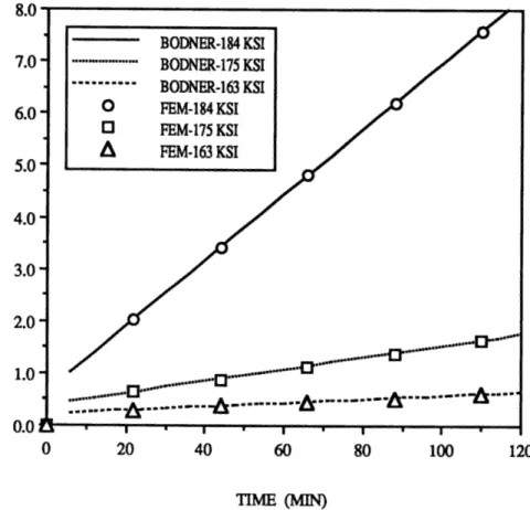
compressive loadings. Bodner's fit of the experimental data for tensile loadings of 163 ksi - 184 ksi is presented in Figure 2.3.1. For these high load cases, the material constants in the internal variable evolution equation result in calculated Rene95 inelastic strain rates that are slightly higher than those seen experimentally.

Table 2.3.1: RENE95 INELASTIC MATERIAL CONSTANTS

Rene95 Constants from Bodner [4]

E = 25.7 x 106 psi v = 0.3

Rene95 Inelastic Constants for Equation 2.2.10 from Bodner [4]

63 = 2 m Do0 < (Z, - a3) exp{ -(a32/ 3 J2) ( (n+l)/n)}

- A

{

(a3 - Zi)/ Z }r

3= = t 3( 3, (Y) psi / sec

n = 3.2 r = 1.5 m = 2.76x 10 psi-1 A = 400.0 x 10-_{6 sec-1} Do = 10.0 x 103 sec- 1 Z, = 319.0x 103 psi Zi = 232.0 x 103 psi (a3)0 = Zi

Figure 2.3.1. B O D N, R [4 ) REN _E95 _ E R I MEN .A L 7 r Tv

i.

C.l) C11 0 0.1 25

30

30 TfMW ("M I

3 FINITE ELEMENT FORMULATION

3.1 Variational Principle

The assumed stress hybrid finite element formulation is derived using the Hellinger-Reissner variational principle by Pian [5]. Assuming that the function is

stationary gives:

8 7R = 0 (3.1.1)

The sum over the entire finite element structure must satisfy this condition.

7CR = _{Y (7R)n (3.1.2)}

The Hellinger-Reissner principle will include both elastic and inelastic strain contributions, however, the inelastic portion will be addressed in a subsequent chapter. The elastic components are written:

- R = 1/2)Sijklijkl " ij ij - Fii i dV

+ Tii i dS + Ti(ui-ui)dS (3.1.3)

where itij is the stress tensor, tij is the strain tensor; iti is the displacement vector, Sijk the elastic compliance tensor, Fi the body force components; and Ti the surface traction.

As pointed out by Fernandez [6] in the derivation of a specialized hybrid solid element, the choice of the Hellinger Reissner variational principle, which

assumes a displacement field throughout the entire element domain, not just on the element boundaries as in the modified complementary energy formulation, means

that one volume integral, rather than several area integrals, need be evaluated. This greatly simplifies the element formulation. In addition, in the element stiffness matrix derivation, the following assumptions are made:

ii

= 0 (no body forces)

Ti = 0 on the boundary (traction free)

ui = ui on the boundary

(3.1.4)

(3.1.5)

(3.1.6)

The Hellinger-Reissner variational principle may then be reduced to:

(3.1.7)

- R = (1/2)Sijk1dijdk1 - dijtij dV

In the assumed stress hybrid finite element formulation the stress tensor is defined as a function of stress parameters, P. In matrix notation the stress is written:

Y = P (3.1.8)

The strain field is written as a derivative of the displacement field in the element which is in turn interpolated from the nodal displacements, q. In matrix notation the strain is written:

where D is a differential operator, and N is the displacement interpolation shape function. The variational principle may now be written in terms of the stress parameters, 0, and nodal displacements, q.

- IR = (1/) (pp)TS(p ) -V - R = (1/2 T pTsPdV -v (P)ITB q dV PT pTBdV q v

The matrices H and G are now defined as:

H = PTSPdV (3.1.

V

G = PTBdV (3.1.

V

The variational principle written in terms of these matrices is:

- R = (1/2) TH -

fTGq

(3.1.

Taking a variation with respect to P results in the following solution for [:

0 = H1Gq (3.1.

The variational principle may be rewritten as:

(3.1.10) (3.1.11) 12) 13) 14) 15)

- R = (1/2) qTGTH-'Gq

This for results in the definition of the finite element stiffness matrix, K, which is written:

K = GTHIG (3.1.17)

The individual element stiffness matrix, defined in terms of the assumed stress field and displacement interpolation field, may be globally assembled to determine the finite element solution to an applied load.

3.2 Eight Node Solid Element

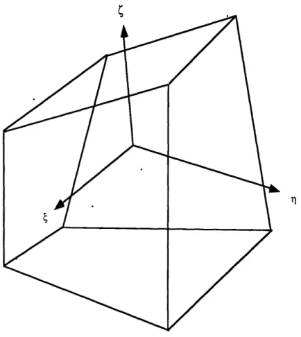
An eight node hexahedral solid finite element is developed by Pian and Tong [7] using an eighteen 0 assumed stress finite element formulation. This element has been programmed in a FORTRAN code by Kang [8] whose subroutines were the basis for the elastic portion of the subsequent analysis verification. For an element of arbitrary geometry as shown in Figure 3.2.1, the stress tensor ij can be written in terms of the natural coordinates 4, i1 and C.

Tll = P1 + 0•i + 09 C + P11 1C (3.2.1) 122 = 02 + 010ý + 12C + 015 r '33 = 03 + +13 + 014T1 + 0161T" T12 = 04 + 017C T2 3 = +5 + 018

s13

=

₀

6

+ 071

These equations give the definition of the stress shape function matrix P.

(3.1.16)

' = P 3 (3.2.2)

The physical components of stress may be obtained using the Jacobian matrix to transform from the natural coordinate system to the Cartesian coordinate system.The stress tensor is written:

aYd = Ai j rij (3.2.3)

where ij is the Jacobian between x,y and z and the natural coordinates 4, 1l and 5. This relationship may also be written in matrix notation as:

a = JT J = JT (P) J (3.2.4)

It should be noted that for this transformation, the Jacobian should be calculated at the element centroid, J (0,0,0), and used for transformation over the entire element, in order for the finite element to pass the "patch" test.

The displacement field is also assumed in the element domain. The interpolation functions may be written in terms of the natural coordinates.

N1 = (1/8) (1 - ) (1 -T) (1 - ) (3.2.5) N2 = (1/8) (1 -) (1 + 1) (1- ) N3 = (1/8) (1 +) (1 +T1) (1-) N4 = (1/g) (1 + 5) (1 - 1) (1 - ) N5 = (1/8) (1 -) (1 -) (1 + ) N7 = (1/8) (1 + 5) (1 + 11) (1 + ) N7 = (1/8) (1 + ) (1 - 1) (1 +) N8 = (1/8) (1+•) (1-Ti) (1+•)

The derivatives of these interpolation functions determine the displacement shape derivative matrix B. The Jacobian matrix is again used to transform from the natural coordinate system to the Cartesian coordinate system in which the nodal

displacements, q, are calculated.

B = J-'DN (3.2.6)

The matrices P and B have been expressed in terms of the stress parameters and the displacement interpolation functions. The matrices H and G are determined by numerical integration over the element domain using Gaussian quadrature, which in turn determines the element stiffness matrix K.

Figure 3.2.1: SOLID ELEMENT OF ARBITRARY GEOMETRY

c:

4 INELASTIC ANALYSIS METHODOLOGY

4.1 Incremental Initial Strain Approach

An incremental initial strain approach to creep and viscoplastic problems using the hybrid stress finite element formulation is presented by Pian and Lee [9]. The Hellinger-Reissner variational principle discussed in chapter 3 may be extended to include inelastic strains as initial strains. For a given time step, the stress rate, oij, and the displacement rate, iii, can be written as stress and displacement increments,

Aoij, Aui. The variational principle may be written as:

-7R = (/2)SijklAoijAakl -AGij i jA ~i-AFiAui dV

V

+ ATiAui dS + ATi(Aui-Aui) dS (4.1.1)

where Aaij is the stress increment tensor; Aeije is the elastic strain increment tensor;, AeijP _{is the inelastic strain increment tensor, Aui is the displacement increments; Sijld} the elastic compliance tensor; AFi the body force increment; and ATi the surface traction increment. Making the same assumptions as in chapter 3, the variational principle reduces to:

-C_R f= f(/ 2)SijklAoijAo kl-AijAijeAijA dV (4.1.2)

V

The stress increment tensor, Ao, is defined as a function of the stress parameter increment, AP3, and the elastic strain increment, Ase , is written in terms of the nodal displacement increment, Aq.

Ao

=

PA3

Aee _{= B Aq}

The variational principle may be rewritten in matrix notation as:

- IR = (1/2) (PA)TS(PA3) - (PA3)TBAq V + (PAP3)TAe dV - =R (1/2) T pTSPdV V + T pTAePdV V

The inelastic matrix GPis defined as:

f

pTAedV

V

The variational principle written in terms of matrices H, G,and GP is:

AfTGAq + A3TGP

Taking a variation with respect to A~3 results in the following solution for AP:

At = H-'(GAq- GP)

The inelastic stress parameter increment is:

(4.1.4) (4.1.5) T f PTBdV q V (4.1.6) (4.1.7) - ER = (1/2) AfTH (4.1.8) (4.1.9) (4.1.3)

AP P = - H-'GP

The inelastic strain, modeled for each time step as an initial strain, is represented in the finite element formulation by the application of a nodal load

increment, AQP.

AQP = GTH-1GP (4.1.11)

For the finite element solution the complete equation for the displacements is:

Aq = K 1 (AQ - AQP) (4.1.12)

The inelastic analysis procedure using a hybrid stress finite element and the Bodner-Partom unified constitutive relations starts by calculating the elastic stress tensor at the element centroid. This stress tensor, and the corresponding deviatoric stress invarient, is used to determine the inelastic strain increment for the first time step. The nodal forces required to treat the inelastic strain as an initial strain are calculated, the applied loading is modified, and the centroidal stress for the subsequent time step is calculated. The stability of the solution depends on the choice of time step in the numerical integration.

4.2 Numerical Integration

The appropriate numerical integration technique and the time step size for the solution of the differential equations governing the material inelastic response is discussed by Haisler and Imbrie [2]. Four numerical integration schemes are considered: explicit Euler forward integration, implicit trapezoidal method,

trapezoidal predictor-corrector method, and Runga-Kutta 4th order method. It is concluded that in terms of accuracy, computational time, and ease of implementation,

a simple scheme such as the Euler method is preferable provided the appropriate time step is chosen.

In the inelastic finite element analysis, the Euler forward integration method is chosen for the numerical integration of the Bodner-Partom evolution equation, determining the growth of the internal parameter, and hence the inelastic strain response of the material. Analysis by Pian and Lee [9] indicates that the appropriate time step increment for a creep problem under a strain hardening rule, such as the Bodner-Partom formulation, is determined by the condition:

AEP At < a (Etotal)time= _t (4.2.1)

where AgP _{is the effective inelastic strain increment, etotal is the effective total strain} at time t, and a is a constant determined by the stability of the problem solution. The effective strain is written:

E = (2/3) (1/2){ ((-11₂₂) +( 22- 33 )2+(ll-33)2

+ (2/3) 3({e 122+-232+C81321 (4.2.2)

The time step optimizer increases the time step as a function of the effective inelastic strain and the effective total strain. For the uniaxial verification of the analysis the value of the constant a was taken to be 0.001.

5 COMPUTATIONAL ANALYSIS VERIFICATION

5.1 Cantilever Beam Analysis

An eight node hexahedral solid finite element using an eighteen 0 assumed stress finite element formulation, as discussed in chapter 3, is used in an inelastic analysis based on the Bodner-Partom unified constitutive relations. The element stiffness matrix formulation is developed by Pian and Tong [7] and programmed in FORTRAN code by Kang [8]. Additional FORTRAN subroutines developed at

MIT [10], "FEABL", are used to assemble the elements and solve the global finite element problem.

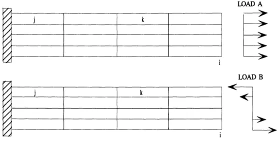
A cantilever beam problem is solved using regular shaped elements (interior angles of 900) with a 5 to 1 aspect ratio, and also using highly skewed elements with minimum interior angles of 140. The finite element model meshes and dimensions

are shown in Figure 5.1.1. Uniaxial tensile and pure shear loadings are applied to the models as shown in Figure 5.1.2. The locations of the elastic finite element

analysis stress and displacement results presented in Table 5.1.1 are also shown in Figure 5.1.2. Under uniaxial tensile loading (Load A), the error in axial deflection

and tensile stress for both the regular and skewed element meshs is negligible compared to the beam theory analytical solution presented by Lindeburg [11]. Under the pure shear loading (Load B), the error in tip deflection and bending stress for the regular shaped element mesh is less 1%, again compared to the beam theory analytical solution. Even in the case of the highly skewed element mesh, where significant errors are expected, the error in tip deflection is less than 5%, and the error in the bending stress is less than 13%. The eighteen [ assumed stress finite element formulation gives satisfactory elastic results to the cantilever beam problem.

The subroutines used for the elastic finite element analysis, together with a subroutine based on the Bodner-Partom unified constitutive relations previously

discussed in chapter 2, were modified and integrated into a FORTRAN code for inelastic finite element analysis. The elastic and inelastic portions of the three dimensional total strain tensor, ij, are calculated from the stress tensor, aij,

evaluated at the element centroid. Based on observations by Haisler and Imbrie [2] a simplified explicit Euler forward integration scheme is used in the integration of the evolution equation. The finite element analysis FORTRAN code is also modified to include a time step optimizer which uses criteria based on the effective total strain, it , and the effective inelastic strain increment, AEP , _{as discussed in chapter 4.}

An inelastic finite element solution to the cantilever beam problem under various uniaxial loadings is calculated using the regular shaped finite element mesh. The Bodner-Partom unified constitutive relation material constants for Rene95 at 12000 F are used for the analysis. The inelastic strain response is presented in Figure 5.3.1. Comparison with Bodner's published Rene95 results, also included in Figure 5.3.1, shows good agreement.

The constant used to calculate the optimum time step increment (a = 0.001

in Equation 4.2.3) was determined by the observation of a stable solution in the initial time steps, particularly for the higher stress loadings. The choice of time step determines the stability of the inelastic strain solution. A more analytical approach to time step optimization based on consideration of the differential equations driving the possible instabilities, is discussed in chapter 6. The inelastic finite element analysis of the uniaxial load case verifies that with the choice of the appropriate time step, or series of time steps, a meaningful solution may be obtained. The computer output for the 175 ksi load case, showing the format of the results presentation, is included in the appendix.

An inelastic solution to the cantilever beam under a uniaxial tensile load of 175 ksi was also calculated using the skewed finite element mesh. A comparison of

element mesh, presented in Figure 5.1.4, shows a significantly different inelastic response despite similar elastic centroidal stress solutions. The regular shaped

element mesh has a faster inelastic strain rate than that calculated using the skewed element mesh, resulting in greater inelastic deflections.

A pure shear load, resulting in a bending stress of 175 ksi at outer layer element centroids, was applied to both regular and skewed cantilever beam element meshes. In this case, the skewed finite element mesh did introduce some error into the centroidal stress solution, on the order of 13% compared to the beam solution. A comparison of the inelastic tip deflection calculated using the regular shaped element mesh to that calculated using the skewed element mesh is presented in Figure 5.1.5. As in the uniaxial load case, the inelastic strain rate calculated using the skewed element mesh has the slower inelastic strain rate.

5.2 Flat Disk Analysis

The inelastic finite element code, verified by comparison with the solution to the cantilever beam problem, is used to calculate the solution to a flat disk under an internal pressure loading. The analytical elastic solution to this plane stress problem is presented by Den Hartog [12]. The flat disk radial and tangential stresses have maximum values at the disk inner radius.

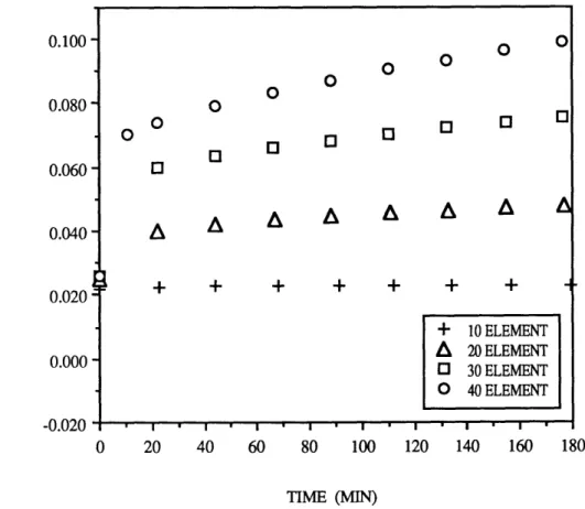
A mesh with five elements covering a 900 arc is chosen, which results in elements that are only slightly skewed, and should eliminate the inaccuracies seen in the shear solution to the cantilever beam problem for skewed elements. In order evaluate the finite element solution, results are calculated for a series of element meshes with increasing element density at the disk inner radius, the location of the maximum stress values. Finite element meshes of 10, 20, 30 and 40 elements and the flat disk dimensions are shown in Figure 5.2.1. The loading (internal pressure)

and finite element boundary conditions are shown in Figure 5.2.2. The elastic radial stress results are presented in Figure 5.2.3, and the elastic tangential stress results are presented in Figure 5.2.4, for the various finite element mesh densities. The finite element results show good agreement with the theoretical solution.

An inelastic finite element analysis using the Bodner-Partom routines and the Rene95 material properties as was used in the cantilever beam problem, is used to calculate the solution to the flat disk problem for the various element mesh densities. The inelastic radial deflection at the disk inner radius is presented in Figure 5.2.5, and the inelastic radial deflection at the disk outer radius is presented in Figure 5.2.6. As expected, the inelastic solution converges as the element mesh density is increased. Since the material inelastic response in this formulation is based on the calculated stress at the element centroid, the denser element meshes, which use the high stresses near the disk inner radius, are needed to correctly calculate the inelastic solution.

Figure 5.1.1: CANTILEVER BEAM ELEMENT MODELS

REGULAR ELEMENT MODEL SKEWED ELEMENT MODEL

IVIIIN AINJLL. = YU ,t.J

LENGTH = 20 IN HEIGHT = 2 IN WIDTH = 2 IN

Figure 5.1.2: CANTILEVER BEAM LOAD CASES

j k

71k

LOAD A

LOAD B NVII " I,+ .iJ.IU.,J

Table 5.1.1: CANTILEVER BEAM ELASTIC RESULTS THEORY* REGULAR FEM SKEWED FEM Displacement at i Load A (ux) Load B (uy) Bending Stress at j Load A (Tx) Load B (Yx) Bending Stress at k Load A (tx) Load B (Yx) 0.1362 in 0.9076 in 175.0 ksi -175.0 ksi 175.0 ksi -175.0 ksi 0.1362 in 0.1362 in 0.9096 in 0.8681 in 175.0 ksi -174.4 ksi 175.0 ksi -173.3 ksi 175.0 ksi -153.3 ksi 175.0 ksi -192.3 ksi * Lindeburg [11]

Figure 5.13_:CAN ER BEAM CI I 1(K) 120 100

120

/

@ i

Figure 5.1.4: CANTILEVER BEAM DEFLECTION (TENSION) 0.50 - 0.400.30 0.20 -20 40 60 80 100 TIME (MIN) 0.10 -0.00 -1 120 . I O REGULAR-175 KSI O SKEWED-175 KSI

Figure 5.1.5: CANTILEVER BEAM DEFLECTION (SHEAR) 1.50 1.40 1.30 -1.20 -1.10 -1.00 0.90 0.80 O REGULAR-175 KSI O1 SKEWED-175 KSI I * I 1 T ' T T 1 20 40 60 80 100 120 TIME (MIN)

-.

Figure 5.2.1: FLAT DISK ELEMENT MODELS

10 ELEMENT MODEL 20 ELEMENT MODEL

30 ELEMENT MODEL 40 ELEMENT MODEL

INNER RADIUS = 2 IN OUTER RADIUS = 10 IN DEPTH = 2.5 IN

Figure 5.2.2: FLAT DISK LOAD CASE

Figure 5.2.3: FLAT DISK ELASTIC RADIAL STRESS -80 -100 -120 -140 -160 -180 -200 0.0 2.0 4.0 6.0 8.0 RADIUS (IN) * Den Hartog [12] 10.0

Figure 5.2.4: FLAT DISK ELASTIC TANGENTIAL STRESS 2.0 4.0 6.0 10.0 RADIUS (IN) * Den Hartog [12]

1

mV"P- I IT ýT T TI 240-220 200 -180 160-140 -120 100-80 -60O 40 -20 -0 A 0.0 -

-Figure 5.2.5: FLAT DISK RADIAL DEFLECTION (INNER)

A

A

A

Ah

+ + + + + + + + 10 ELEMENT A 20 ELEMENT O 30 ELEMENT O 40 ELEMENT I.I.I.a.I. I 0 20 40 60 80 100 120 140 160 180 TIME (MIN) 0.100 0.080 0.060 - 0.040-0.020 0.000--0.020 q

Figure 5.2.6: FLAT DISK RADIAL DEFLECTION (OUTER)

0 0

0]

A

A

o + + + + + + + + 10 ELEMENT A 20 ELEMENT o 30 ELEMENT O 40 ELEMENT 0 20 40 60 80 100 120 140 160 180 TIME (MIN) 0.0220.020 0.018 - 0.016-0.014 0.0120.010 -n -n-nQ 0.006 -0.004 -0.002 -0.000 --0.002 I -I 1 ' I ' 1 · 1 ' I ' I ' I ' 1 r 41 11

6 DISCUSSION

6.1 Finite Element Solution

In the finite element analysis of the cantilever beam problem is seen that, although the elastic solution of stress and displacement has negligible error for both the regular shaped element mesh and the skewed element mesh, there is a significant difference in the inelastic solution results. The inelastic strain is treated as an initial strain in the inelastic analysis formulation. This requires incrementally updating the load applied at each time step to compensate for the inelastic deformation The amount of the change in load is calculated by integration, Gaussian quadrature, of the change in inelastic strain, AeP , over the element volume. For the cantilever beam models the location of the element centroid is the same, however, due to the element shape, the Gaussian point locations will be different with respect to the beam

geometry. This difference may account for the differences seen in the inelastic results.

The flat disk problem may be used to comment on the finite element mesh density required to calculate a valid stress field and a meaningful problem solution. The four meshes of increasing element density accurately calculate the elastic radial and tangential stresses. The accurate calculation of the centroidal stress is important; under the present inelastic analysis formulation, the element inelastic strain response is dependant on the centroidal stress only. For the flat disk problem the denser element meshes are required to get the element centroid close enough to the peak stress to allow for the correct inelastic material response.

An alternative to a fine mesh finite element analysis is the modification of the inelastic analysis to use the Gaussian integration point stress results to determine the inelastic response. This will require internal variable information for each

accuracy of the sub-element solution and allow the use of coarser finite element meshes.

6.2 Inelastic Solution Stability

The stability of the inelastic finite element solution is dependant on the numerical integration of the time dependant differential equations, e.g. the internal variable evolution equation (Eq. 2.2.10). In the inelastic finite element solution of

the cantilever beam under uniaxial loading, an instability was observed in the inelastic strain response for the high stress load cases. This necessitated the choice of a relatively small constant in the time step optimizer criteria in order to get a valid

solution (a = 0.001 for the unified inelastic formulation, compared to the constant used by Pian and Lee [9], a = 0.05 for a power law creep formulation).

It was noted, however, that even with the much smaller constant, the finite element solution becomes unstable. At a relatively high time, the inelastic strain begins to increase without bound. This is not due to an instability in the numerical integration of the internal variable evolution equation, however. At the time step the the instability occurs, which can be identified in the cantilever beam problem by a departure from the expected solution, the internal variable, %,3, has already reached the saturation value, Z1. The internal variable, %3, becomes a constant and the inelastic strain rate then becomes a function of stress only; a function that is described by equations 2.2.7 and 2.2.8. The change in inelastic strain rate is written:

kigp _{= tijP(J2,sij) (6.2.1)}

AEP

= AeP(Aa)

The inelastic analysis formulation treats the inelastic strain response of previous time steps as an initial strain problem (the load vector Q, and the stress field parameter vector 0, are modified). The stress field is a function of the stress field parameter vector increment, A[ P.

AU = P AD = AG(A3 P) (6.2.3)

The parameter vector increment, A[ P, is a function of the inelastic strain as

described by equations 4.1.7 and 4.1.9, equations which include the integration of the inelastic strain rate over the time interval.

Ap P = A[ P(eP ) _(6.2.4)

This series of relationships defines a differential equation for the inelastic strain.

0P = OP(O) = 0P(f3P) = OP(eP) (6.2.5)

An approach for the derivation of an appropriate numerical integration scheme, and a corresponding rational selection of time step increment is given by Zienkiewicz et al [13]. The algorithm presented includes an adaptation to nonlinear problems, such as the problem presented by the finite element inelastic strain calculation. The implementation requires the interpolation of the finite element parameter values over the time step using a polynomial expansion and obtaining higher order derivatives. The polynomial expansion allows an estimation of the

of the time step, or time step increment may be set. The task of implementing this approach into the inelastic finite element analysis, the numerical integration, and the time step optimization is considered a subject for future work.

6.3 Inelastic Material Property Definition

One of the most difficult tasks in undertaking an inelastic analysis using the unified constitutive model is the definition of the material properties. The Bodner-Partom model uses an internal variable to represent material isotropic hardening. In an evaluation of Rene95 material properties, Bodner [4] discusses the physical interpretation of the parameters of his model, and arrives at the set of material constants presented in chapter 2, and used in the finite element analysis. The inelastic material behavior of Rene95 at 12000 F has also been investigated by

Stouffer et al [14]. The experimental data for the high stress loadings is compared to Bodner's material constant calculated results in Figure 6.3.1. Experimental Rene95 minimum inelastic strain rates (secondary creep) for various loadings is presented in Figure 6.3.2. It is noted that the data presented by Stouffer shows consistently higher strain rates.

The Rene95 experimental data presents the opportunity to modify the material constants of the Bodner-Partom unified constitutive model to reflect a different set of data. The procedure would begin by fitting a set of isochronous inelastic material response curves. Each of the material constants in the internal parameter evolution equation affect this response as described in chapter 2. Several of the constants, such as n, r, A and Do, can be assumed to be near the Rene95 values, as they affect the shape of the curves rather than the magnitude. Through the appropriate choice of the internal parameter limits, Zi, the internal parameter at the initial state, Z1, the internal parameter at the saturation value, and m, a coefficient of the internal parameter rate equation, the isochronous curves may be fit. A similar

procedure would be used to fit experimental data of Rene95 at other temperatures, and to fit the experimental data of other materials.

6.4 Gas Turbine Blade Application

The proper modeling of the inelastic behavior of a material is critical in the analysis of aircraft engine hot section components, and in particular gas turbine blades. The stress rupture, or creep, characteristics of a blade often determine the functional life of the part. The finite element analysis presented in earlier chapters is only the first step toward applying a unified constitutive relation approach to blade life analysis. The inelastic analysis procedures used here need to be expanded to address body forces, temperature dependant material properties, and thermal stresses. There are, however, classes of turbine blade problems that may use

simplifying assumptions allowing analysis as the finite element formulation expands. The incorporation of body forces into the finite element formulation would allow analysis of uncooled LPT turbine blades. These blades are typically thin, shrouded airfoils running at a relatively uniform temperature across a span. A finite element model of a shrouded airfoil is shown in Figure 6.4.1. Because of a uniform bulk temperature, the thermal stresses are small and may be neglected. For a

conservative analysis, the material temperature dependance may also be neglected as the area of concern is the stress and inelastic response of the hotter upper portions of the airfoil and of the shroud.

Material property temperature dependance and thermal stresses become important in the analysis of cooled turbine blades. When cooled at all, LPT turbine blades are lightly cooled, and the temperature for a particular span is still relatively constant. An example of a cooled LPT blade finite element model is shown in

and although the thermal stress may sometimes be neglected, the temperature dependance of the material properties may not.

Finally, in the analysis of highly cooled HPT turbine blades, there are very high thermal stresses that, although over time may relax out, can significantly affect the inelastic behavior, and hence the creep life of the blade. It is this class of problems that is historically the most important from the point of view of the engine designer, and the most difficult to analyze. The incorporation of expanded

capabilities of body forces, temperature dependant material properties, and thermal stresses into the inelastic finite element formulation would provide a useful tool in the design of turbine blades.

6.4 Future Work

First, there are steps that may be taken to improve the accuracy and stability of the present inelastic finite element analysis formulation. The numerical integration scheme may be updated from the Euler forward method to the algorithm proposed by Zienkiewicz [13]. This allows a measure of the error in the numerical integration, and provides an analytical method for determining the appropriate time step increment necessary to maintain solution stability.

The Bodner-Partom unified constitutive model is one of many unified models currently proposed. Although satisfactory for a isothermal steady-state analysis, models such as the one proposed by Walker [15] which include a "back stress" term in the internal variable evolution equation, allowing kinematic

hardening, are necessary to model correctly the response to changing loads. As mentioned in the discussion of the application to gas turbine blade analysis, the incorporation of body forces to represent the centrifugal loading, temperature dependant material properties to appropriately model the material response in areas of temperature gradients, and thermal stress capability to calculate

the affect on creep life in areas of high thermal stress are features necessary for a practical design tool.

Figure 6.3.1: STOUFFER [14] RENE95 EXPERIMENTAL RESULTS

0

00 []r

enseme ememme1 mm1 ea mesmam memesm memmes ammesm ememam

10 15 20 25 30 TIME (MIN) 4.0-3.01 BODNER-184 KSI BODNER-175 KSI ... _{BODNER-163 KSI} O EXP-184 KSI O] EXP-175 KSI A EXP-163 KSI 2.0 -

1.0-0.0

0 It_I a : a . a I ir U I I I I 5.0 i - I i I "

Figure 6.3.2: RENE95 EXPERIMENTAL INELASTIC STRAIN RATE O 0O 0

SB

0 0 0 0 0 0 BODNER [4] EXPERIMENTAL 0 STOUFFER [14] EXPERIMENTAL I I l ' l I l I i I*I lI ' 110 120 130 140 150 160 170 180 190

APPLIED STRESS (KSI) 10 -6

7 CONCLUSION

Inelastic finite element analysis has been developed using eight node solid assumed stress hybrid finite elements for definition of the stress field, the Bodner-Partom constitutive relations for definition of the inelastic strain response, and an

incremental initial strain approach to calculate the inelastic stress and strain response through time. Evaluation of fundamental cantilever beam problems using Rene95 inelastic material constants, verifies the elastic and inelastic finite element solutions. Highly skewed finite elements are seen to affect the inelastic strain response in the beam problems, reducing the inelastic strain and inelastic strain rate as compared with a regular shaped finite element mesh.

The solution of a flat disk problem using finite element models of increasing mesh densities used to evaluate a multi-axial load case. Although the elastic solution of centroidal stress in satifactory for all the meshes, the inelastic solution is

dependant on the element centroidal stress only, so denser element meshes are necessary to get the element centroid close enough to the inner radius peak stress to allow a correct calculation of the inelastic response. The use of the stress state at the element Gaussian integration points for the inelastic strain calculation is one possible solution to this problem.

The stability of the inelastic solution is seen to be a function of numerical integration technique and the time step increment chosen. The constant required in

the time step optimizer for the unified constitutive inelastic analysis required to maintain a stable solution is seen to be more than an order of magnitude smaller than the constant used in a traditional power-law creep finite element analysis. An analytical approach to time step increment selection, such as that proposed by Zeinkiewicz, would improve the stability of the solution.

The analysis of gas turbine blades requires an expansion of the current formulation to address centrifugal and thermal loading, and temperature dependant material properties. Incorporation of these capabilities, and the development of unified constitutive material constants for a variety of other materials, would provide a useful tool in the evaluation of turbine blade designs.

REFERENCES

[1] Chan, K.S., U.S. Lindholm, S.R.Bodner and K.P. Walker, "A Survey of

Unified Constitutive Theories", Second Symposium on Nonlinear Constitutive

Relations for High Temperature Applications, NASA Lewis Research Center, 1984.

(NASA CP-2369)

[2] Haisler, W.E. and P.K. Imbrie, "Numerical Considerations in the Development and Implementation of Constitutive Models", Second Symposium on Nonlinear

Constitutive Relations for High Temperature Applications, NASA Lewis Research

Center, 1984. (NASA CP-2369)

[3] Bodner, S.R. and Y. Partom, "Constitutive Equations for Elastic-Viscoplastic Strain Hardening Materials", Journal of Applied Mechanics, 42, 2, 385-389 (1975).

[4] Bodner, S.R., "Representation of Time Dependant Mechanical Behavior of Rene95 by Constitutive Equations", Technical Report, Air Force Materials Laboratory, 1979. (AFML TR-79-4116)

[5] Pian, T.H.H., "Nonlinear Creep Analysis by Assumed Stress Finite Element Methods", AIAA Journal, 12, 12, 1756-1758 (1974).

[6] Fernandez, J.A.G., "Hybrid Solid Elements with a Traction Free Cylindrical Boundary", SM Thesis, Massachusetts Institute of Technology, 1986.

[7] Pian, T.H.H. and P. Tong, "Relations Between Incompatible Displacement

Model and Hybrid Stress Model", International Journal for Numerical Methods in Engineering, 22, 173-181 (1986).

[8] Kang, D.S., "Solid Hybrid Element -8 Node, 24 DOF", FORTRAN Code, Massachusetts Institute of Technology, 1983.

[9] Pian, T.H.H. and S.W. Lee, "Creep and Viscoplastic Analysis by Assumed Stress Hybrid Finite Elements", Finite Elements in Nonlinear Solid and Structural

Mechanics, (Ed. P.G. Bergan et al), Norwegian Institute of Technology, 2,

807-822 (1977).

[10] MIT, "FEABL", FORTRAN Code, Massachusetts Institute of Technology, 1983.

[ 11] Lindeburg, M.R., (Ed.), Mechanical Engineering Review Manual (7th

Edition), Professional Publications Inc., Belmont, CA, 1984.

[12] Den Hartog, J.P., , Advanced Strength of Materials, McGraw-Hill, NY, 1952.

[13] Zienkiewicz, O.C., W.L. Wood, N.W. Hine and R.L.Taylor, "A Unified Set

Of Single Step Algorithms, Part 1: General Formulation and Applications",

International Journal for Numerical Methods in Engineering, 20, 1529-1552 (1984).

[14] Stouffer, D.C., L. Papernik and H.L. Bernstein, "An Experimental Evaluation of the Mechanical Response Characteristics of Rene95", Technical Report, Air Force

[15] Walker, K.P., "Research and Development Program for Nonlinear Structural

Modeling with Advanced Time-Temperature Dependant Constitutive Relationships", Final Report, NASA Lewis Research Center, 1981. (NASA CR-165533)

O in Itooo c'i 0 .4 In rr F4 0 r%a'18 a i

. ll I

K

Di

i

ii'

00f000000QOO0000:0000:03:0000000:

"k00 000000000 0000 0 00000000 000~00000 I'*

* °"

•°

i

+++*+*°+~*++

K "M C; C;U ;C ;ýC ;0C ;C ;C ;ZC ;4 ;C ;C ;C ; N'wa _{+i a} S 0. 4 00. 00000@ I

I

*P eh

I

'4 H

i a m o 0 0000000000 0000000000 0000000000 St0 IP00 C

I

huuhe~uuhhE

44.. 1- C4 I-10 _{,,,.,,°°,w~u}i onooooooooo 14SU4.MNMMMWM6NM

P Cooo oooo oooooo00000000000 oooooo ooo"oooooo 00 oosoooo~oooooooooooooogoooooo~ooooooo 0093000~~o 00 ocoo0000000 0 0 0 So 0@ 0 00:00o 00900000000000~ 00000000000000000000000000000000000:00000000:000ccoo 00 0000000000000000000000000cc0a*0000a00000000000 • 00000000000000000000000000000000000000000000000 00 0 00 000000000000000000000000000000000000000 0000000000 0:000000300000000000000 mOOr((mnlOOr( 000000000000000000000000000000000000000000000 00 0 000000000000000000 000 0000000000000000 0000000000000000000000000000000000000000000000 000000000000000800000000000000000000000000000000000 * ooooo~ooooooooooooooooooo nooonmoo • 4 A ri vao nn a i -m m a a 00000000000000ma000

(Orn coo MOM 000 * *B. " Ii a,l wOe .04 6+o NON I o 3 333 MM9 Iý aI Iý.04 6+ NON NON 0oIS NOC 000 I III 3 A33

AmNo

.40.4 i+ WOo 000 Co. .40.4_IDOIa 6+i WOW e.4 o0.4 coo I I f- o r'-K 4 0 4 Wa vnI Am. t-Ol. .40.4₆₊₆ M' 1.Ot-In1 ain 000; C OOOO"""" 00000000_~++++6 666 0000.4..4._OOOOrn... 0 3 I 00000000 C! ! ÷C1" 11 4 " papi ohm oooo I I II I I I I 141 1414 KM 14 14 ll 0 Ioo•N DDDDDDDD * 000 o Inn owoooo 0 o Oo I O IN O 000 +I I I II III III Mu 0 000 _{a s 00000000}Wwwoww DDDDDDDD ft v3 00000000 W4 coo +4 "

* u

++Mill+ I iO 00000000 t u i Illlll0I0 I

a

oldI

W 000+ * 000 _{6 6O} 0000_{WW O W} PI i ilql l llilI1 l * ~I:B _{* O} 133113 IIKH 0 000I 600 00 600 6 NO 6 00 600 too too SIn too 61-0 I I K 6+1 14MM I-I Noo 6 6 3 333B~ A A AAY S Yi a *Q morl .40.4 6+ Mil 000_WOW r.•O6 NON I I I E E S ~ 0000 N N N N 00000000 ++++

OCOM""

6666 ooo06 Ir6 i 0000.4.4.4.4 @00 C! 000 Vcooo_{I i+}

cooo I|1 |11I

.4 000 9MM W vow oo??oooo,,o I I ~ I Y CY~l( W O .40W0a0W4aW0 0 000 666 66 66 .o. ooooooo O 000 ,,,,,,SW 6 6O6 _{C- l} OVOOOWOOO_{4.V4 N4 NW .4 N4 N4} * vow 00000000 ft c o IIII I I I I W" 141 1I IIIII O O 00000000 .4 000 + I +I 0N 000 O ₀ 000 00000000 30 O000

eis,-0I:::::

+ 6+

rtarari

00 oo 614O I N 6.4O 666 I 1.o r-..404 000_,+';' coo 00000000 0000co4..4.4 00 00 CUO oil 00000000 fill ,,,,, , O ON DDD0D0 .4 000 • ~R,roo,,,no r. oMoo. WWNN-W.o * WOW A. 4 ,04r.400 .4 000 66666666 0 000 Newwowww ,,, 6oooooWo,, 111 I 00000000 14 ' 0 NoN _oooYY(rl(( D"99~ o noo o•,•,oo.. r4 000 =

IIII

,,,,,,,,~r I I l 900 46o1 400.4400.4 0I vOw 00000000 P) 000 6++ 6+ 6 6O S OS OO ro oo0" ,,,,, ,,, 00 0l33 0 110000 I 111 000000001 10 "on ~~~~ O 000 + 0 bll+ I ( Y~n~ I @00K rl ceI a Itw IcwP~~iat mI-m I 6o 'OO I N Il60600₆₁₃ 65 60 60 60 6* 60 63 66 63 00 600 6 0 600 600_6.o0 o! 600 too 600 II I I I 600 6100 noo :o I6

I"

U(OU 0.4 CDl 0oa coo M i0-4 000 I 6 WONo 6+6 MNi r. 0 °. aOOO 000 I I II MM MbTM1 NON i+I clr o vooWOW 000 * LII) N YNNN ~4 b4is" r- 0 r-.06 1+6 .No nonr ._40.ONor• coo I III

@6ON a0' sOOOeOON00000000

N40 M ++++ II oo000 0000 r-f a0000a.4..4.=4 C! 0 0000000 ! 0 NON• 00°0.0 .4 000 w WOW .-...00.. O 000 OOOOOOOOI O 000 I oI I 0 I0 I A cow ooooo t.o V -.V ° 1.Nv V I I 00o00o000 I I I I I M I i 000 i M N Nx ONNMMMMT Wako of+ ,00% 600 (00 6*** 600_oo 800 s • Iin₆₀₀100_{S O} I U

is

,m

88_{6 U} aN OOOONNNN *coooo(y +M+"III o 0000.445. 00 00 N P M aoo 0a M MM . . .ý .4! .9 •!4! I0 00000000 a 000 aooocooo N TooT so "' N NN* N 10 ago coocoooo NMil n IO 00000000 In 00 00000000 4.0 I I I I 00000000 • • • in C0 4Y M I I M l0 II x °x C o l i a oi - a ov-oovwo + 6+6)~~) NICllc 0 MK Q11YM Y in 00CMO me- Ye *.NC6 4PawmseI-e Boco P t oo00 I*c INc oo 600 601 Ioooo 600 00 IN I U IN |r o"I M 1+1040+ o 000 I +I h o o coo I III " NN" o r 0 -6 6+6 * 000 00000000000NNNN 88M ++ AatA 0000 v-88 cooccruee I co I I I| 0 oo 00000086o "! "t0e! A I I I A t a g S000 p 14 00000000 VO co I I ooooo o yoN oooooooo O N ! I _Il " ONOONOO 000 + I i oo * vOW 00000000 o *ooo II 60 000 in Doo n me-N morn e0at ouy~~n Nj N NNNN 600 o** 500 Ioa I ccmo MI I _IIW I611 o00 oo 800oo_n00 • . 6NO mo 6--6.40 100600

iC

IM 6I*

I+5 S B U.N lm so. .40. so. .40.4 000_{I i} A | A I I 3UN cc+ v a OW OO 000 000.01.4. C0000... 000 Bo ÷,. ,, N N 505 00000000

ooo 00 0 oOoo•"0 olr, ISIBIBBcooo 0aO4 q q•

oo.. ...

,, ,

BB00000000 33300000000 .4 ....IIWII1|11I11h11 II 000 S'1 mNN 505 .0.4.400..00000000 Ilk, oil,:::: 000 +0000000 cooo I l l i • .. wsqquS4uu

III oooooooo_l1Ililll

000 ZOOO_1+! S S 00 0 coo ?+1+_{N N '44N44} * 3 00000000

i

°" "

_"

* INr ii,,.i. 000 000 50010 19 . coo commommum a _{N 0 5: NON 000}cooo_{545 f} Cddd ++ 0 n 000on O B00am33 4i U.N; 100 BNO ! 0₀₀ I

I

c

1

IS

SN ace_@0 I+ In 0 In 1 1 ?o? S(0P. 50_+~

t..o nonaIn

Pom noo AOPf a000C I I 1 l '4 14Oa V4 woo' 1+ ' (0(4 ++ *+ AA 0 000 _O o _{0 0 0'} o _4OOOOO .4NON :;cocoonI_00005555~r S 00000000•o OO 1111-111O " `1C - t" A,,,,,,on n o 0 OOWW::Wv:: ',4 COIO '4 000 DDDDDD0 P. 0i 00000000 00o. .o.o.o.oo N 00 . I 914mm"OI S000000:S14_{11 B00000000} +1 I S+N I S S I ooo I I I OOOOOOOO N NNN 1191.471111 SMOPS 00000000 PS 505 00000000 Nomi O *@@ +++++.+ " N°" HII1 n h"* 0 000 NN,.d.,N.,. I I 0 0000000 ISISiSIS l l o ! _oooi OIIII Ik I I₃I N l* * lli** * o00 I Ioo In 0 I I loO 00 S O IN I

ii

now O '40'4 + I Sol CooMoo? PS ! OP i ++9 II. " no oooo•oo 0co000oooo oooo•=rt0t 0000...0000. I I I llll O N~oN DPDDPDDD I min...₀ ow 00000000 '0001 1 U MUM 'I al llSl:alala OfD I o0i 00000000 goo

coo

v vo 000 0000SSS O oo000 O00OOO I I ovW(ooWO I II ooooooo 3113 00000000 gI I Il l + _{4 '000}I+l 4; C; 4; C;, 5 50 00000000 P. 000 *SI+,SI mmm"oow 31310 I 0011000 0 00li" PS 00Cm *~ A P. rlY~n 3, NON 4dPSSN PIBISISS mmr hOO 3*d 5** 5 03033 3Mn U M l~ NN KNBU + I ! rl DYO| IV acer K4 N0NN * 000 04V 000o a coo rft r. 0 rf ,+1 S S B * III~ KMM Cd NON ._{0 000}rloP. 00 OOO NY BNK O 000 I III_OPC! a4 '40. •i - _I

aM

r IO(N D I I + I is net? 4 '4 000 r. mo0 o d ddd =_{co I} S00 P. _I cdoo4_{I1II o} I 0 coo I 4!. `1ONi O 000 0 0 1 _10CY0 SIn 5n a 0 + I + I tl , OOO a 0 0 i4 11 ₀₀₀0 C

f'i:

W~la sosP 500 too 100 S.. , C40 500 100 1o IPS_{: c°} Soo B.o IPS II I I mi 1 1 10 S B I r-to