Publisher’s version / Version de l'éditeur:
Information Bulletin on Variable Stars, 6201, 2017-03-17
READ THESE TERMS AND CONDITIONS CAREFULLY BEFORE USING THIS WEBSITE.
https://nrc-publications.canada.ca/eng/copyright
Vous avez des questions? Nous pouvons vous aider. Pour communiquer directement avec un auteur, consultez la première page de la revue dans laquelle son article a été publié afin de trouver ses coordonnées. Si vous n’arrivez pas à les repérer, communiquez avec nous à [email protected].
Questions? Contact the NRC Publications Archive team at
[email protected]. If you wish to email the authors directly, please see the first page of the publication for their contact information.
This publication could be one of several versions: author’s original, accepted manuscript or the publisher’s version. / La version de cette publication peut être l’une des suivantes : la version prépublication de l’auteur, la version acceptée du manuscrit ou la version de l’éditeur.
For the publisher’s version, please access the DOI link below./ Pour consulter la version de l’éditeur, utilisez le lien DOI ci-dessous.
https://doi.org/10.22444/IBVS.6201
Access and use of this website and the material on it are subject to the Terms and Conditions set forth at
BN pegasi: a semidetached eclipsing binary
Nelson, Robert H.
https://publications-cnrc.canada.ca/fra/droits
L’accès à ce site Web et l’utilisation de son contenu sont assujettis aux conditions présentées dans le site LISEZ CES CONDITIONS ATTENTIVEMENT AVANT D’UTILISER CE SITE WEB.
NRC Publications Record / Notice d'Archives des publications de CNRC:
https://nrc-publications.canada.ca/eng/view/object/?id=8258d597-3001-41e8-9942-a7d471609a63 https://publications-cnrc.canada.ca/fra/voir/objet/?id=8258d597-3001-41e8-9942-a7d471609a63
COMMISSIONS G1 AND G4 OF THE IAU INFORMATION BULLETIN ON VARIABLE STARS
Volume 63 Number 6201 DOI: 10.22444/IBVS.6201
Konkoly Observatory Budapest
17 March 2017 HU ISSN 0374 – 0676
BN PEGASI – A SEMIDETACHED ECLIPSING BINARY
NELSON, ROBERT H.1,2
11393 Garvin Street, Prince George, BC, Canada, V2M 3Z1, email: [email protected]
2Guest investigator, Dominion Astrophysical Observatory, Herzberg Institute of Astrophysics, National
Re-search Council of Canada
The variability of BN Peg (AN 145.1935; NSVS 14426159; TYC 537-44-1), amongst many others, was discovered photographically by Hoffmeister (1935) who gave coordinates, a magnitude range, and a finder chart, and described the system as an Algol. Jensch (1935) supplied elements (epoch, period) and 15 photographic eclipse timings. Mallama (1980) and Kreiner (2004) presented up-to-date elements. Over the years, there have been a number of eclipse timings, but no light curve analysis.
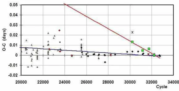
Light curve and radial velocity data have been acquired, but before any analysis, the first task was to examine the period variation. An eclipse timing difference (O-C) plot using all available data is reproduced in Figs. 1 and 2.
Figure 1. BN Peg – eclipse timing (O-C) diagram with fits to primary and secondary eclipse timings. Legend: small squares – photographic; triangles – visual; filled circles – photoelectric; filled diamonds – CCD. The four large squares are secondary minima (PE and CCD). The asterisk symbols are rejected
Figure 2. BN Peg – eclipse timing (O-C) diagram, identical to Fig. 9 but in more detail.
It will be seen that the many points since the first (in 1929) display considerable scatter. While the scatter is understandable for the photographic and visual points display, it is not clear why the photoelectric (PE) and CCD points are not more consistent. One possibility is that the system is undergoing an elliptical orbit with apsidal motion due to a third body. If that is the case, some of the supposedly deviant points would fit together with the other secondary minima to obey a different relation – that depicted in more detail in Fig. 10. (The first secondary minimum may still be deviant, however, and was not included in the fit of Fig. 10.) Also, the period may be changing over the long term, and there may even be a short-term cyclic component. However, all this is very speculative; future eclipse timings will be required to settle the matter. The eclipse timing (O–C) Excel file may be found online at Nelson (2016).
Although both the spectroscopic and photometric data were taken at about cycle 32 000, it seemed the safest procedure (in view of the scatter) to take the best-fit for the primary eclipse data from cycle 25,500 to the present. Small errors in the slope should not affect the phasing significantly. The result, equation (1) was used for all phasing.
JD(Hel) MinI = 2457254.7346 + 0.7132973E (1) In July-August of 2015, the author took 145 frames in V , 146 in RC (Cousins) and 161
in the IC (Cousins) band at his private observatory in Prince George, BC, Canada. The
telescope was a 33 cm f/4.5 Newtonian on a Paramount ME mount; the camera was a SBIG ST-10XME. Standard reductions were then applied. The variable, comparison and check stars are listed in Table 1. The coordinates and magnitudes for all three stars are from the Tycho Catalogue (Hog et al. 2000).
In October of 2015 and again in September of 2016, the author then took a total of 9 medium resolution (R∼10000 on average) spectra of BN Peg at the Dominion Astro-physical Observatory (DAO) in Victoria, British Columbia, Canada using the Cassegrain spectrograph attached to the 1.85 m Plaskett Telescope. He used the 21181 grating with 1800 lines/mm, blazed at 5000 ˚A giving a reciprocal linear dispersion of 10 ˚A/mm in the first order. The wavelengths ranged from 5000 to 5260 ˚A, approximately. A log of observations is given in Table 2. The following elements were used for both RV and
IBVS6201 3
Table 1: Details of variable, comparison and check stars.
Object GSC RA (J2000) Dec (J2000) V (mag) B − V (mag) Variable 0537-0044 21h28m04.s27 04◦ 59′ 01.′′ 97 10.84(7) +0.43(10) Comparison 0537-1042 21h28m32.s20 04◦ 57′ 53.′′ 99 10.55(6) +0.97(11) Check 0537-0899 21h29m00.s79 05◦ 00′ 57.′′ 50 10.59(6) +0.70(10)
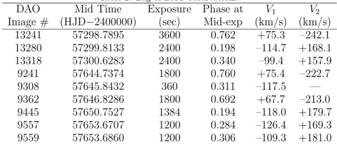
Table 2: Log of DAO observations.
DAO Mid Time Exposure Phase at V1 V2
Image # (HJD−2400000) (sec) Mid-exp (km/s) (km/s)
13241 57298.7895 3600 0.762 +75.3 –242.1 13280 57299.8133 2400 0.198 –114.7 +168.1 13318 57300.6283 2400 0.340 –99.4 +157.9 9241 57644.7374 1800 0.760 +75.4 –222.7 9308 57645.8432 360 0.311 –117.5 — 9362 57646.8286 1800 0.692 +67.7 –213.0 9445 57650.7527 1384 0.194 –118.0 +179.7 9557 57653.6707 1200 0.284 –126.4 +169.3 9559 57653.6860 1200 0.306 –109.3 +181.0 photometric phasing:
Frame reduction was performed by software ‘RaVeRe’ (Nelson 2009). See Nelson et al. (2014) for further details.
Radial velocities were determined using the Rucinski broadening functions (Rucinski 2004; Nelson 2010b; Nelson et al. 2014). An Excel worksheet with built-in macros (written by him) was used to do the necessary radial velocity conversions to geocentric and back to heliocentric values (Nelson 2010a). The resulting RV determinations are also presented in Table 2. For the 2015 data, the results were corrected 2.2% and 1.0% up, respectively, to allow for the small phase smearing. (Because of the shorter exposure times possible with the newly-coated optics, no correction was necessary for the 2016 data.) Correction was achieved by dividing the RVs by the factor f = (sinX)/X; where X = 2πt/P , where t denotes exposure time and P denotes the orbital period. For spherical stars, this correction is exact; in other cases, it can be shown to be close enough for any deviation to fall below observational errors. The mean rms errors for RV1 and RV2 were 4.2 and
7.7 km/s, respectively, and the overall rms deviation from the (sinusoidal) curves of best fit was 6.5 km/s. The best fit yielded the values K1 = 98.7(3) km/s, K2 = 208.6(7) km/s
and Vγ = –22.6(4) km/s, and thus a mass ratio qsp = K1/K2 = M2/M1 =.0.473(2).
The author used the 2003 version of the Wilson-Devinney (WD) light curve and radial velocity analysis program with Kurucz atmospheres (Wilson and Devinney 1971; Wilson 1990; Kallrath et al. 1999) as implemented in the Windows front-end software WDwint (Nelson 2009) to analyze the data. To get started, the spectral type F5 (taken from SIMBAD, no reference given; main sequence assumed) was adopted. Interpolated tables from Cox (2000) gave a temperature T1 = 6650 ± 300 K and log g = 4.355 ± 0.020. (The
quoted errors refer to two and one half spectral sub-classes.) An interpolation program by Terrell (1994, available from Nelson 2009) gave the Van Hamme (1993) limb darkening values; and finally, a logarithmic (LD=2) law for the limb darkening coefficients was
se-Table 3: Limb darkening values from Van Hamme (1993) for T1 = 6650 K and T2 = 4221 K. Band x1 x2 y1 y2 Bol 0.640 0.548 0.243 0.266 V 0.705 0.781 0.280 0.260 RC 0.632 0.749 0.287 0.297 IC 0.548 0.664 0.275 0.309
lected, appropriate for temperatures < 8500 K (ibid.). The limb darkening coefficients are listed below in Table 3. (The values for the second star are based on the later-determined temperature of 4248 K and assumed spectral type of K6.) Convective envelopes for both stars were used, appropriate for cooler stars (hence values gravity exponent g = 0.32 and albedo A = 0.500 were used for each).
From the GCVS 4 designation (EW) and from the shape of the light curve, mode 2 (detached) was used. Early on, it was noted that the maxima between eclipses were unequal. This is the O’Connell effect (Davidge & Milone 1984, and references therein) and is usually explained by the presence of one or more star spots. Because Max II (phase 0.75) was lower than Max I (phase 0.25), a solution was first obtained with a spot added to star 1. (Later on, a solution was sought with the spot on star 2 but it gave poorer residuals than the one for star 1, so the former was adopted.)
Convergence by the method of multiple subsets was reached after a considerable num-ber of iterations. (The subsets were: (a, e, L1), (ω, T2, q), (Vγ, Ω2). and (e, i, Ω1). The
spots were handled separately.)
Detailed reflections were tried, with nref = 2, but there was little–if any–difference in the fit from the simple treatment. There are certain uncertainties in the process (see Csizmadia et al. 2013; Kurucz 2002). On the other hand, the solution is very weakly dependent on the exact values used.
In the first set of iterations when the fit was near, the sigmas for each dataset were adjusted, based on the output of WD (viz. computed from the sum of residuals for each dataset plus number of points). To aid in comparison between different solutions, the same sigmas were then used throughout the different trails.
Despite multiple trials, no completely satisfactory solution could be reached in mode 2 with T1 = 6650 K. (The fit for the secondary eclipse in the I band was poor.) A better
solution was achieved by assuming an earlier spectral type, that of F2, with a temperature of T1= 7000 K (Cox 2000). Designate these as solutions A and B, respectively. Additional
considerations (see later discussion) suggested that mode 5 (Algol) should be investigated. Trials therefore were made with mode 5 at the same two temperatures. Solution D with T1 = 7000 K was unsatisfactory, but solution C with T1 = 6650 K stood out from all the
rest for a number of reasons to be discussed later.
All four models are presented in Table 4. Note that estimating the uncertainties in temperatures T1 and T2 is somewhat problematic. A common practice is to quote the
temperature difference over–say–1.5 spectral sub-classes (assuming that the classification is good to one spectral sub-classes, the precision being unknown). In addition, various different calibrations have been made (Cox 2000, pages 388-390 and references therein, and Flower 1996), and the variations between the various calibrations can be significant. (Flower gives T1 = 6542 K for F5 for example.) However, there is an additional
un-certainty here because a spectral type (for star 1) is assumed to be F2. Therefore, a larger uncertainty, that of two and one half spectral sub-classes is adopted here, giving
IBVS6201 5
an uncertainty of ± 300 K to the absolute temperatures of each. The modelling error in temperature T2, relative to T1, is indicated by the WD output to be much smaller, around
20 K.
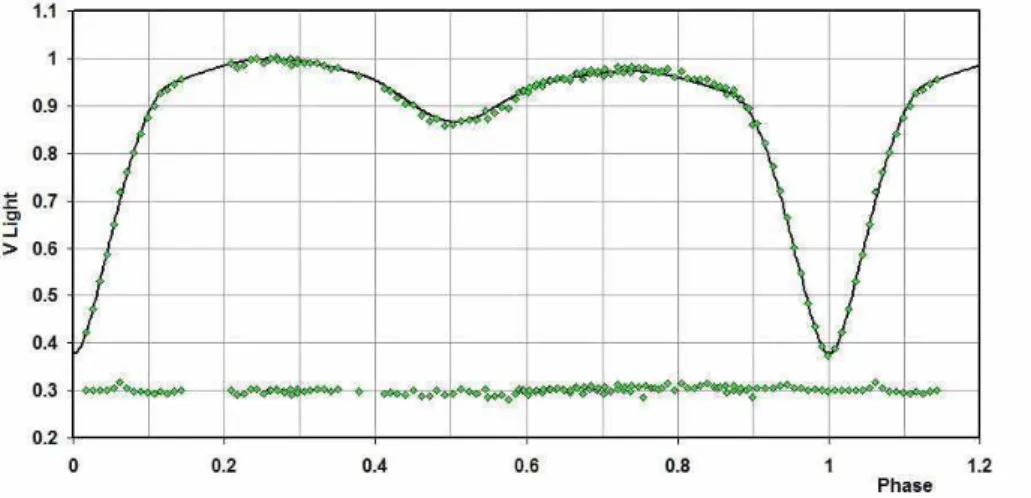
Figure 3. V light curves for BN Peg (solution C) – data, WD fit, and residuals.
Figure 4. Rlight curves for BN Peg (solution C) – data, WD fit, and residuals.
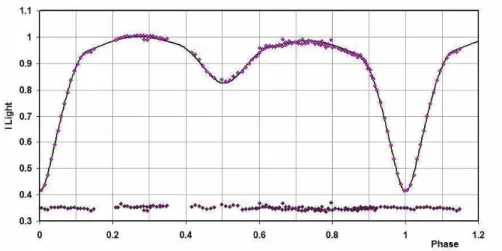
The light curve data and the fitted curves for solution C are depicted in Figures 3–5. The residuals (in the sense observed-calculated) are also plotted, shifted upwards by 0.30, 0.35, and 0.35 units, respectively.
The radial velocities and the fit of solution C are shown in Fig. 6. A three-dimensional representation from Binary Maker 3 (Bradstreet 1993) is shown in Fig. 7.
The WD output fundamental parameters and errors are listed in Table 5. Most of the errors are output or derived estimates from the WD routines. From Kallrath & Milone (1999), the fill-out factor is f = (ΩI − Ω)/(ΩI − ΩO), where Ω is the modified Kopal
potential of the system, ΩI is that of the inner Lagrangian surface, and ΩO, that of the
Figure 5. I light curves for BN Peg (solution C) – data, WD fit, and residuals.
Figure 6. Radial velocity curves for BN Peg – data and WD fit.
IBVS6201 7
Table 4: Wilson-Devinney parameters.
Solution >> A B C D
WD Quantity value value value value error unit
Mode 2 2 5 5 — — Spectral type F5 F2 F5 F2 — — Temperature T1 6650 7000 6650 7000 [fixed] K Temperature T2 4248 4388 4221 4389 20 K q = m2/m1 0.490 0.505 0.486 0.505 0.004 — Potential Ω1 3.108 3.133 3.159 3.175 0.008 — Potential Ω22 2.901 2.944 2.881 2.903 0.008 Inclination, i 83.4 83.5 82.6 82.2 0.1 deg
Semi-maj. axis, a 4.59 4.61 4.59 4.61 0.06 sol. rad. Syst. velocity, Vγ −22.0 −20.8 −20.8 −20.8 1.8 km/s
Eccentricity, e 0.006 0.006 0.014 0.008 0.001 — Phase shift 0.0028 0.0028 0.0023 0.0025 0.0003 —
Arg. periastron, ω 19.2 19.1 17.6 19.8 0.1 deg
Spot co-latitude 81 75 79 75 10 deg
Spot longitude 74 78 81 78 5 deg
Spot radius 27.4 27.4 34.9 27.4 4 deg
Spot temp. factor 0.9659 0.9650 0.9793 0.9650 0.0020 — L1/(L1+ L2) (V ) 0.9475 0.9472 0.9460 0.9417 0.0002 —
L1/(L1+ L2) (RC) 0.9222 0.9243 0.9195 0.9169 0.0003 —
L1/(L1+ L2) (IC) 0.8952 0.8991 0.8911 0.8897 0.0004 —
r1 (pole) 0.3777 0.3762 0.3707 0.3707 0.0004 orb. rad.
r1 (point) 0.4329 0.4320 0.4205 0.4216 0.0008 orb. rad
r1 (side) 0.3946 0.3930 0.3862 0.3864 0.0005 orb. rad.
r1 (back) 0.4116 0.4103 0.4020 0.4026 0.0006 orb. rad.
r2 (pole) 0.2914 0.2917 0.2944 0.2987 0.0003 orb. rad.
r2 (point) 0.3756 0.3695 0.4216 0.4274 0.0017 orb. rad
r2 (side) 0.3032 0.3033 0.3068 0.3115 0.0003 orb. rad.
r2 (back) 0.3324 0.3313 0.3389 0.3438 0.0005 orb. rad.
P
ω2
Table 5: Fundamental parameters.
Solution >>> A B C D
Quantity value value value value Error unit
mode 2 2 5 5 — — Temperature, T1 6650 7000 6650 7000 300 K Temperature, T2 4248 4338 4221 4389 300 K Mass, m1 1.717 1.723 1.725 1.723 0.05 M⊙ Mass, m2 0.841 0.870 0.839 0.870 0.004 M⊙ Radius, R1 1.81 1.82 1.78 1.78 0.02 R⊙ Radius, R2 1.42 1.43 1.45 1.47 0.02 R⊙ Mbol,1 2.88 2.66 2.93 2.70 0.1 mag Mbol,2 5.36 5.21 5.35 5.14 0.1 mag Log g1 4.16 4.16 4.18 4.17 0.01 cgs Log g2 4.06 4.07 4.04 4.04 0.02 cgs Luminosity, L1 5.8 7.1 5.5 6.9 0.5 L⊙ Luminosity, L2 0.59 0.68 0.60 0.72 0.05 L⊙ Fill-out factor 1 −0.86 −0.822 −1.06 −0.96 0.10 — Fill-out factor 2 −0.15 −0.20 0 0 0.10 — Distance, r 354 394 345 389 35 pc
To determine the distance r, the analysis (using solution C) proceeded as follows: First the WD routine gave the absolute bolometric magnitudes of each component; these were then converted to the absolute visual (V ) magnitudes of both, MV,1 and MV,2, using the
bolometric corrections BC = −0.140 and −0.984 for stars 1 and 2 respectively. The latter were taken from interpolated tables constructed from Cox (2000). The absolute V magnitude was then computed in the usual way, getting MV = 3.02 ± 0.20 magnitudes.
The apparent magnitude in the V passband was V = 10.84 ± 0.07, taken from the Tycho values (Hog et al. 2000) and converted to a Johnson magnitude using relations due to Henden (2001). The colour excess (in B−V ) was obtained in the usual way, by subtracting the tabular value of B − V (for that spectral class) from the observed (converted Tycho) value. This gave E[B −V ] = −0.07 magnitudes which is not physically possible. However, reference to the dust tables of Schlegel et al. (1998) revealed a value of E[B − V ] = 0.063 for those galactic coordinates. Since the E[B − V ] values have been derived from full-sky far-infrared measurements, they therefore apply to objects outside of the Galaxy; this value of E[B − V ] so derived then represents an upper limit for closer objects within the Galaxy. Hence the lower value of half that, 0.032 is reasonable, and was adopted. (An uncertainty of–say–half this amount was used in the error calculation for distance.)
Galactic extinction was obtained from the usual relation AV = R E[B − V ], using R
= 3.1 for the reddening coefficient. Hence, for solution C, a distance r = 345 pc was calculated from the standard relation:
r = 100.2(V −MV−AV+5)
pc (2)
The errors were assigned as follows: δMbol,1 = δMbol,2 = 0.01, δBC1 = 0.020, δBC2 = 0.330
(the variation of 2.5 spectral sub-classes), δV = 0.07, δE(B−V) = 0.10, all in magnitudes, and δR = 0.1. Combining the errors rigorously (i.e., by adding the variances) yielded an estimated error in r of 35 pc.
IBVS6201 9
= 6650 K) gives a primary mass, radius and luminosity that are too large for the zero age main sequence (ZAMS) values listed in column 3 (Cox, 2000). Reference to the evolutionary tables of Schaller et al. (1992, solar type, mass 1.7 solar masses, their table 16) reveals that the temperature of T1 = 6650 K is too low to fit the terminal age main
sequence (TAMS) or any evolved state. Solution A is therefore rejected.
Turning to solution B (detached, F2, T1 = 7000 K), one might believe that star 1
started with a higher temperature on the TAMS but cooled as it evolved. However, reference to the same evolutionary tables (ibid) reveals that, for an age of 1.3 Gy, the temperature would fit, but then the actual luminosity at 7.1 L⊙ would be too small for
their computed value of 11.3 L⊙. For this reason, we reject solution B.
Solution C (Algol, F5, T1 = 6650 K) fits better because temperature T1 matches the
assumed spectral type, the mass ratio matches the spectrographic value, and the sum of residuals squared is the lowest of the four solutions. Also, most importantly, Solution C makes sense because Algols are known to have experienced mass flow from the secondary (but originally more massive star) to its companion. That would explain the excess mass for the F5 star. Its larger radius would then account for the higher luminosity. Therefore we adopt solution C (mode 5, Algol) as the correct one.
In conclusion, the fundamental parameters of this system have been determined, albeit to a somewhat lower level of precision than one would like. It is to be hoped that higher precision data from a planned remote site with routine photometric skies plus a renewed classification will confirm the exact nature of this system.
Acknowledgements: It is a pleasure to thank the staff members at the DAO (especially Dmitry Monin and David Bohlender) for their usual splendid help and assistance.
References:
Bradstreet, D.H., 1993, “Binary Maker 2.0 - An Interactive Graphical Tool for Preliminary Light Curve Analysis”, in Milone, E.F. (ed.) Light Curve Modelling of Eclipsing Binary Stars, pp 151-166 (Springer, New York, N.Y.)
Cox, A.N. 2000, Allen’s Astrophysical Quantities, 4th ed., (Springer, New York, NY) Csizmadia, S., Pasternacki, T., Dreyer, C., Cabrera, A., Erikson, A., Rauer, H., 2013,
A&A, 549, A9 DOI
Davidge, T.J., Milone, E.F., 1984, ApJS, 55, 571 DOI Flower, P.J., 1996, ApJ, 469, 355 DOI
Henden, A., 2001, http://www.tass-survey.org/tass/catalogs/tycho.old.html Hoffmeister, C. von, 1935, AN, 255, 401 DOI
Høg, E., et al., 2000, A&A, 355, L27 Jensch, A. von, 1935, AN, 255, 417 DOI
Kallrath, J., Milone, E.F., 1999, Eclipsing Binary Stars–Modeling and Analysis (Springer-Verlag)
Kallrath, J., Milone, E.F., Terrell, D., Young, A.T., 1998, ApJ, 508, 308 DOI Kreiner, J.M., 2004, AcA, 54, 207
Kurucz, R.L., 2002, Baltic Astron., 11, 101 Mallama, A.D., 1980, ApJS, 44, 241 DOI
Nelson, R.H., 2009, Software, http://www.variablestarssouth.org/profilegrid blogs/software-by-bob-nelson/
by-bob-nelson/
Nelson, R.H., 2010b, “Spectroscopy for Eclipsing Binary Analysis” in The Alt-Az Initia-tive, Telescope Mirror & Instrument Developments (Collins Foundation Press, Santa Margarita, CA), R.M. Genet, J.M. Johnson and V. Wallen (eds)
Nelson, R.H., 2016, Bob Nelson’s O-C Files, http://www.aavso.org/bob-nelsons-o-c-files Nelson, R. H., S¸enavcı, H.V. Ba¸st¨urk, ¨O., Bahar, E., 2014, New Astron., 29, 57 DOI Rucinski, S. M., 2004, IAUS, 215, 17
Schaller, G., Schaerer, D., Meynet, G., Maeder, A., 1992, A&AS, 96, 269 Schlegel, D.J., Finkbeiner, D.P., Davis, M., 1998, ApJ, 500, 525 DOI Terrell, D., 1994, Van Hamme Limb Darkening Tables, vers. 1.1. Van Hamme, W., 1993, AJ, 106, 2096 DOI
Wilson, R.E., Devinney, E.J., 1971, ApJ, 166, 605 DOI Wilson, R.E., 1990, ApJ, 356, 613 DOI