HAL Id: hal-00799119
https://hal-enpc.archives-ouvertes.fr/hal-00799119
Submitted on 11 Mar 2013HAL is a multi-disciplinary open access archive for the deposit and dissemination of sci-entific research documents, whether they are pub-lished or not. The documents may come from teaching and research institutions in France or abroad, or from public or private research centers.
L’archive ouverte pluridisciplinaire HAL, est destinée au dépôt et à la diffusion de documents scientifiques de niveau recherche, publiés ou non, émanant des établissements d’enseignement et de recherche français ou étrangers, des laboratoires publics ou privés.
The transportation sector and low-carbon growth
pathways: modeling urban, infrastructure and spatial
determinants of mobility
H. Waisman, Céline Guivarch, Franck Lecocq
To cite this version:
H. Waisman, Céline Guivarch, Franck Lecocq. The transportation sector and low-carbon growth pathways: modeling urban, infrastructure and spatial determinants of mobility. Climate Policy, Taylor & Francis, 2013, 13 (1), pp.106-129. �10.1080/14693062.2012.735916�. �hal-00799119�
1
The transportation sector and low-carbon growth pathways:
1modelling urban, infrastructure
2and spatial determinants of mobility
3Henri Waisman*,†, Céline Guivarch*,**, and Franck Lecocq*,*** 4
5
*Centre International de Recherche sur l’Environnement et le Développement
6
(CIRED, ParisTech/ENPC & CNRS/EHESS)
7
45bis avenue de la Belle Gabrielle 94736 Nogent sur Marne CEDEX, France.
8 9
**École Nationale des Ponts et Chaussées—ParisTech,
10
6-8 avenue Blaise Pascal – Cité Descartes, Champssur Marne, 77455 Marne la Vallée, France.
11 12
*** Agro Paris Tech 13
16 rue Claude Bernard F-75231 Paris Cedex 05, France
14 15 16 17 18 19 20 21 †
2
The transportation sector and low-carbon growth pathways:
1introducing urban, infrastructure and spatial determinants
2of mobility in an E3 model
3Abstract 4
There is still a controversy as to the effect of spatial organization on CO2 emissions. This 5
paper contributes to this debate by investigating the potentials offered by infrastructure 6
measures favoring lower mobility in the transition to a low-carbon economy. This is done by 7
embarking a detailed description of passenger and freight transportation in an energy-8
economy-environment (E3) model. In addition to the standard representation of transport 9
technologies, this framework considers explicitly the “behavioural” determinants of mobility 10
that drive the demand for transport but are often disregarded in mitigation assessments: 11
constrained mobility needs (essentially commuting) imposed by the spatial organization of 12
residence and production, modal choices triggered by installed infrastructure and the freight 13
transport intensity of production processes. This study demonstrates that the implementation 14
of measures fostering a modal shift towards low-carbon modes and a decoupling of mobility 15
needs from economic activity significantly modifies the sectoral distribution of mitigation 16
efforts and reduces the carbon tax levels necessary to reach a given climate target relatively to 17
a “carbon price only” policy. This result is robust to a wide range of assumptions about 18
exogenous parameters. 19
Keywords: transport, mitigation policy, infrastructure, spatial organisation 20
JEL: C68, O18, R40 21
3
1 - Introduction
1
2
Curbing emissions in the transportation sector is a major issue for any ambitious climate 3
policy. Carbon emissions from transport activities have indeed experienced a fast growth 4
(+44% over the past two decades) to reach 22.5% of all energy-related (IEA, 2011a), and are 5
expected to pursue this trend in the future (for example,(IEA, 2011b) predicts a further 6
increase by one-third by 2030). This trend is not incompatible with ambitious climate policies 7
as long as the reductions of global emissions can be obtained by exploiting low-cost 8
mitigation potentials in residential, industry and power sectors (IPCC, 2007, Figure SPM6). 9
But, at a long-term horizon, the drastic reduction of carbon emissions made necessary by 10
low stabilization targets cannot be reached without controlling also transport-related 11
emissions. 12
A large body of literature explores mitigation options and policies in the transport sector and 13
emphasizes that ambitious reductions in the transport sector would require actions on both 14
the “technology” side to decrease both the energy intensity of transportation modes and the 15
carbon content of fuels, and on the “behaviour” side to reduce the volume of mobility and 16
foster the adoption of low-carbon modes. This diagnosis contrasts with existing analyses of 17
the transport sector with energy-economy-environment (E3) models, which are useful tools 18
to investigate the role of transportation in the transition to a low-carbon economy, given the 19
important interactions between transportation and the rest of the economy. However, these 20
approaches remain limited to explore the full mitigation potentials of the transport sector 21
because they have essentially focused on the assessment of the “technology” side (e.g. 22
Schafer et al., 2009). To provide a more comprehensive vision, these tools have to be 23
4
complemented with representation of the “behavioural” determinants of transportation 1
dynamics (Schafer, 2012). 2
This paper is an attempt to bridge the gap between studies of mitigation options and policies 3
in the transport sector and E3 models. It first reviews the literature on climate policies and 4
the transportation sector, to delineate the determinants and obstacles to CO2 emissions
5
reduction in that sector (section 2.1) and emphasize the potential role of policies on the 6
“behaviour” side of transportation dynamics (section 2.2). Section 3 describes how stylized 7
representations of the “behavioural” determinants are introduced in the E3 model Imaclim-8
R (Waisman et al., 2012) to explicitly represent the interplay between transportation, energy 9
and growth patterns when accounting for the rebound effect of energy efficiency 10
improvements on mobility, endogenous mode choices in relation with infrastructure 11
availability, the impact of investments in infrastructure capacity on the amount of travel, and 12
the constraints imposed on mobility needs by firms’ and households’ location. This 13
framework is then used in Section 4 to assess the role of transportation in low-carbon 14
pathways. 15
This analysis demonstrates the risk of high losses if using carbon price as the sole 16
instrument, and investigates the potentials offered by richer combination of measures. 17
Complementarily to carbon pricing, this study considers more specifically actions to control 18
the ”behavior” determinants of transportation in the course of the low-carbon transition, 19
including (i) spatial reorganizations at the urban level and soft measures towards less 20
mobility-dependent agglomerations, (ii) reallocation of investments in favor of public modes 21
at constant total amount for transportation infrastructure and (iii) adjustments of the 22
logistics organization to decrease the transport intensity of production/distribution 23
processes and optimize the use of vehicles. This analysis provides a first step towards the 24
5
identification of non-energy determinants of global mitigation costs and concludes with a 1
roadmap for further integrating transportation, housing and urban dynamics issues into 2
macroeconomic assessment of climate policies. 3
. 4
2 - Climate policies and the transportation sector
52.1 Determinants and obstacles of carbon emission reductions in the transport sector 6
As it is standard in climate analyses, we decompose transport carbon emissions along its 7
four essential determinants: the carbon intensity of fuels, the energy intensity of mobility, 8
the modal structure of mobility and the volume of mobility. Following Chapman (2007) and 9
Schafer (2012), the first two determinants can be labeled as “Technology”, while the last two 10
can be labeled as “Behaviour”. 11
12
Technology 13
The carbon intensity is dependent on the primary sources used to produce the final energy 14
used to fuel vehicles. Today, the vast majority comes from oil refining, but anticipations of 15
resource depletion and oil price increases make credible the large-scale diffusion of other 16
sources at a medium-term horizon. The decrease of fuels’ carbon intensity then crucially 17
depends on the potential of low-carbon processes for liquid fuel supply (biofuels) and on the 18
diffusion of alternative energy carriers (electricity and hydrogen). All these low-carbon 19
options are faced with intrinsic limitations. 20
Biofuels raise three types of concerns, which may limit their large scale diffusion. First, the 21
technical potential of biomass production remains controversial and difficult to characterize 22
6
due to large uncertainty on yield improvements, the production potential of degraded land 1
and climate change feedbacks (Chum et al., 2011). Second, the lifecycle impact of biomass 2
on GHG emissions may be less beneficial than expected with respect to conventional fuels, 3
depending on the use of fertilizers, the input of fossil fuels in the production, transport and 4
conversion of biomass, as well as on how land use is affected by the biomass production (see 5
Searchinger et al., 2008; Tilman et al,. 2009). Third, large scale biomass production is 6
submitted to land-use and water-use competition with other usages and objectives like food 7
provision, timber production or forest conservation. Nuclear and renewables, the main 8
carbon-free power technologies, are limited by political acceptability and intermittency, 9
respectively. Competitive and safe hydrogen storage systems with the appropriate end-user 10
infrastructure face important technological obstacles. Put together, all these obstacles 11
highlight the risk that the supply of long-term end-use energy for transport may rely 12
importantly on particularly carbon-intensive options (non-conventional oil, gas-to-liquids 13
and coal-to-liquids) driving fastly growing trends of these sources to reach 7.4 mb/d in 2030 14
according to IEA projections (IEA, 2011b) 15
The energy intensity of mobility results from the technical characteristics of the vehicle fleet 16
for which improvements may be limited by asymptotes on technical progress of drive train 17
efficiency and inertias on the deployment of new energy-efficient vehicles. Indeed, the 18
market potential may be only a fraction of its economic potential if, under partial 19
information and imperfect foresight about the future of energy costs (Allcott, 2010; 20
Anderson et al, 2011; Allcott, 2011), purchase decisions under-value or even ignore future 21
energy savings of vehicle efficiency (Greene, 1998; Turrentine and Kurani, 2007) and are 22
importantly influenced by other considerations than energy consumption (e.g., safety, 23
performance, size). Standards have proven efficient to foster the diffusion of more carbon 24
7
efficient vehicles (around 140gCO2/km), but their effect at more stringent constraints may 1
be limited in absence of clear price-signals allowing an appraisal of long-term benefits in 2
terms of energy savings. 3
Behaviour 4
The modal structure of mobility breaks down between carbon-intensive options (air, 5
passenger cars, trucks) and low-carbon ones (public transport and non-motorized modes for 6
passengers; rail, shipping and inland waterways for freight). The promotion of the latter 7
group requires dedicated investments in infrastructures for public modes to improve their 8
coverage, speed, reliability and flexibility. Yet, in absence of intermodal synergies, 9
cumulative mechanisms such as positive network externalities often make it cheaper to 10
expand one network instead of maintaining two in parallel (e.g., rail + road), especially when 11
accounting for inertias in the renewal of long-lived infrastructures. Therefore path-12
dependencies and lock-ins in energy-intensive mobility options may arise. 13
14
The volume of mobility results from households’ tradeoffs between passenger transport and 15
the demand for other goods under budget and time constraints, as well as firms’ freight 16
mobility needs in the production/distribution process. These decisions are constrained by 17
the interplay between four effects, each of them imposing inertia on the dynamics of 18
mobility. First, passenger daily commuting distances and the transport intensity of 19
production are defined by the spatial distribution of housing, transport and industrial 20
infrastructures, which are long-lived and hence characterized by strong inertias. Second, 21
location choices, and hence mobility needs, are decided in function of a tradeoff between 22
transport and housing expenditures. The decrease of transport prices in real terms (ie with 23
8
respect to income) combined with an increase of housing prices are at the root of urban 1
sprawl triggering a rise of mobility needs (Brueckner, 2000). These trends could be reversed 2
only if the dynamics of transport and housing sectors are reversed. Third, in line with the 3
seminal work by (Zahavi and Talvitie, 1980) confirmed by more recent studies (Metz, 2008; 4
Schäfer et al, 2009; Schäfer, 2012), households are conventionally assumed to devote a 5
given time to mobility so that speed gains permitted by infrastructure deployment may give 6
rise to increased distances (longer daily travels and more occasional trips) and modal shifts 7
(in favor of fast modes within the time constraint, like aviation). Finally, the tradeoff 8
between inventories and just-in-time organizations decides the logistics organization and in 9
particular the total vehicle-kilometers travelled for the production/distribution of a given 10
volume of goods (McKinnon, 2010; Piecyk and McKinnon, 2010). 11
Moreover, two well-known feedback effects apply to the volume of mobility (Hymel et al., 12
2010). On the one hand, the “induced demand effect” (Goodwin, 1996) is a response to 13
infrastructure building or improvement, which may trigger an increase of mobility because 14
of enhanced accessibility or improved services provided by a given mode. In the long run, 15
enhanced accessibility also changes the economic value of land, affecting the locations of 16
activities and housing and hence mobility needs (Noland, 2008). The influence of the 17
“induced demand effect” on CO2 emissions is described in Shalizi and Lecocq (2009) for the
18
case of the US Interstate Highway. On the other hand, the “rebound effect” captures the 19
increase of mobility consecutive to reductions of the marginal costs of travel permitted by 20
fuel economy under improved efficiency (Greening et al, 2000). The magnitude of this effect 21
can be very significant: for instance, Wang et al. (2012) estimate that the average rebound 22
effect for passenger transport by urban households is around 96%, indicating that the 23
9
majority of expected reduction in energy consumption (and CO2 emissions) from efficiency
1
improvement could be offset. 2
3
This general picture illustrates that changes in transportation patterns are driven by other 4
crucial determinants than energy prices such as income, the spatial organization, housing 5
costs and transport infrastructure availability. 6
7
2.2 Mitigation policies in the transport sector 8
A very large literature explores mitigation options and policies in the transport sector at 9
different spatial scales. The most recent publications include studies at the global scale (e.g. 10
IEA, 2009; Schafer et al., 2009; Johansson, 2009), at the regional level (e.g. Banister, 2000 for 11
Europe), at the national scale (e.g. Bristow et al., 2008, for UK; Akerman and Hojer, 2006, for 12
Sweden; Mc Collum and Yang, 2009, and Greene and Plotkin, 2011 for US) and at the city 13
scale (e.g. Hickman et al., 2010 for London; Hickman et al., 2011 for London and Delhi). All 14
these studies share the conclusion that technologies (reducing the carbon intensity of 15
energy and the energy intensity of transport modes) will play a major role. However, the 16
majority of studies also conclude that actions on the modal structure and volume of mobility 17
(grouped under the label “behavior”) will be required; the extent of these actions depending 18
on the technological optimism of the study. 19
Besides the issue of the relative importance of actions on the “technology” side vs. actions 20
on the “behavior” side, the question of the policy instruments to trigger emissions 21
reductions is central. 22
10
2.2.1 Price signals, energy demand and carbon emissions
1
A crucial specificity of the transportation sector is that demand for transportation services, 2
and fuel consumption from vehicles appear weakly sensitive to energy prices. This appears 3
clearly in (Goodwin et al. 2004), who estimate a low value of short-run price elasticities for 4
the traffic volume (-0.1) and fuel consumption (-0.25).The higher short-run price elasticity 5
for fuel consumption than for the traffic volume captures that unitary fuel consumption per 6
miles traveled can decrease even in the short-term thanks to a more efficient use of 7
vehicles, including eco-driving.1 This study also demonstrates that price elasticities are 8
greater by factors of 2–3 over five-year periods, but also that income elasticities are greater 9
than price elasticities by factors of 1.5–3. These general conclusions are confirmed by more 10
detailed recent analyses. By distinguishing econometric estimates of long-run price 11
elasticities for gasoline and diesel demand, for different price and income levels and for 120 12
countries, (Dahl, 2012) obtains that price elasticities range between -0.11 and -0.33, and 13
between -0.13 and +0.38 for gasoline and diesel respectively, while income elasticities are 14
much higher (between +1.26 and +0.66 for gasoline and around +1.34 for diesel). This means 15
that, even at a long term horizon, fuel consumption reductions triggered by price increases 16
may be offset by wealth effects, especially in fast growing economies. 17
This review demonstrates that only a sustained increase of price signals in the very long run 18
is likely to affect significantly transport-related carbon emissions. However, only high carbon 19
prices would trigger a notable increase of fuels’ end-use price. For instance a price of carbon 20
of 40-100 $/CO2—in the very high range of what is currently considered feasible at large
21
scale—would translate in a moderate 0.35–0.90 $ per gallon increase in gasoline cost. 22
Looking forward, the IPCC thus estimate that multiplying the price of carbon by 5 in 2030 23
11
(from 20$/tCO2 to 100$/tCO2) would only induce a 23% decrease of transport-related carbon
1
emissions (IPCC, 2007). 2
2.2.2 The role of mobility-control measures
3
A direct implication from the above review is that, under a “carbon-price-only policy”, 4
substantial mitigation in the transportation sector can be reached only through very high 5
carbon prices. This diagnosis is confirmed by studies on marginal abatement costs curves in 6
the transport sector compared to other sectors, which demonstrate that mitigation options 7
in the transport sector are mainly towards the right of MACCs, i.e. with high carbon prices 8
(e.g. UK Committee on Climate Change, 2008; Smokers et al., 2009). The concerns raised by 9
the political acceptability and the economic consequences of such high carbon prices lead to 10
consider the role of complementary measures that aim at controlling transport-related 11
carbon emissions through specific actions. 12
Number of measures can be envisaged to decrease the carbon intensity and/or the energy 13
intensity determinants of carbon emissions, but all of them are submitted to constraints 14
limiting their efficiency. For instance, the development of electric (or hydrogen) vehicles 15
faces important technological barriers and dedicated and coordinated policies would be 16
necessary to favor their diffusion, including basic research and R&D, infrastructure 17
deployment (e.g., charging stations) and pricing incentives. For what concerns energy 18
intensity, standards (such as fuel efficiency or carbon emissions standards) help to overcome 19
private agent’s partial information and imperfect foresight when making vehicle purchase 20
decisions and have been the most effective way of reducing transportation emissions since 21
the 70’s (particularly recently with EU regulations to automakers). However, the future 22
potentials of this option may be limited by saturation of efficiency potentials in mature 23
12
fleets, inertias due to the political economy of tightening standards and the slow renewal of 1
vehicles’ fleet (notably in developed countries). 2
Because of these obstacles, it appears necessary to consider specific measures on the 3
“behavior” determinants of transport-related emissions, namely mobility volume and 4
structure. To reduce overall demand for transportation, some degree of reorganization of 5
firms’ production/distribution process and households’ patterns of consumption is necessary 6
(McKinnon, 2010; Piecyk and McKinnon, 2010; Bristow et al., 2008). Both are closely 7
dependent upon the spatial organization of the economy. In fact, concentration of 8
production units as well as their location with respect to consumption areas is crucial 9
determinant of the volume and modes of freight transport necessary for production. 10
Moreover, households’ mobility is strongly constrained by the necessity to access to 11
essential activities and especially to commute for work purpose. The latter is strongly 12
correlated with the spatial organization of human settlements, and especially with the 13
development patterns of urban areas (according to (UN, 2011), 77% of population in 14
industrialized world live in urban areas, whereas this percentage is about 46% in developing 15
countries and is expected to increase rapidly over the next decades). Many econometric 16
studies have demonstrated that energy consumption (and CO2 emissions) from transport are
17
correlated with population density or other more precise city morphological indicators 18
(measuring city shape, accessibility to public transport, etc) (Mindali et al., 2004; Bento et 19
al., 2003; Grazi et al., 2008; Le Néchet, 2011). Several case studies discuss the hypothesis of 20
the compact city as a sustainable urban form (Holden and Norland, 2005; Muniz and 21
Galindo, 2005) and the association between automobile dependence (or emissions) and land 22
use planning and regulations (Newman and Kenworthy, 1996; Glaeser and Kahn, 2010). 23
Moreover, developing public transport network to favor modal shift is beneficial if the 24
13
density of settlements is sufficient. This means that a voluntarist reorientation of 1
investments towards public modes cannot but be associated with policies that affect 2
households and firms locations (notably land-use policies, fiscal policies to control land 3
markets etc.) (Shalizi and Lecocq, 2009). 4
Complementary policies on the demand side should thus include infrastructure policies, 5
fiscal policies, land-use policies, building regulations and other policies affecting how 6
buildings are designed, but also industrial policies and other regulations that affect how 7
firms locate. In addition to these “physical policies” (i.e. policies dealing with a physical 8
infrastructure element), “soft policies”, in particular those replacing physical mobility by 9
telecommunications, should be considered (see Cairns et al. 2004; Anable et al., 2005; Cairns 10
et al., 2008; Santos et al., 2010). 11
12
3 - Modeling the transport-energy-economy nexus of mitigation costs
13The points made above are by no means new discoveries and were already evident when 14
climate emerged as a major issue in the late 80s. One could then expect that modeling 15
frameworks developed to assess the costs of climate policies would have embarked the 16
specificities of the transportation sector through joint frameworks between energy, 17
transportation and urban dimensions (Hourcade, 1993). However, the overwhelming 18
majority of energy-economy-environment (E3) models conventionally used to assess 19
mitigation costs reveals a methodological lock-in towards a focus on energy at the detriment 20
of an explicit representation of transport dynamics and adopt carbon price as the only driver 21
of decarbonizing economies (IPCC, 2007). Of course, the transportation sector is not absent 22
from these models but most of them still lack an explicit representation of the non-price 23
14
drivers and lifestyles (recent steps in this direction include (Anable et al., 2012) and (Brand et 1
al., 2012). 2
Schafer (2012) offers an overview of the state of the art of transportation representations in 3
E3 models, and calls for the introduction of behavioral change into these models. This means 4
bridging a gap between (i) bottom-up technology-rich models, which rely on exogenous 5
trends of transportation demands, and therefore have no endogenous evolution of modal 6
choices or mobility volumes, and (ii) top-down macroeconomic models, which 7
conventionally represent the transportation sector in nested CES (constant elasticity of 8
substitution) production functions, so that demand changes are exclusively price-induced. 9
Moreover, none of these two types of models can account for the “rebound effect” 10
following technology improvement nor for the “induced demand effect” following 11
infrastructure development. 12
We adopt the E3 model Imaclim-R (Waisman et al, 2012), which belongs to the family of 13
models trying to bridge the gap between bottom-up and top-down models and to introduce 14
to various extent non-energy and non-price drivers of transportation dynamics (see Schafer, 15
2012 for an overview). 16
17
3.1 General architecture of the IMACLIM-R model
18
The hybrid dynamic general equilibrium model IMACLIM-R proposes a framework that helps 19
disentangling the role of transport in long-term socio-economic trajectories and the 20
potentials offered by specific measures on this sector for mitigation costs. 21
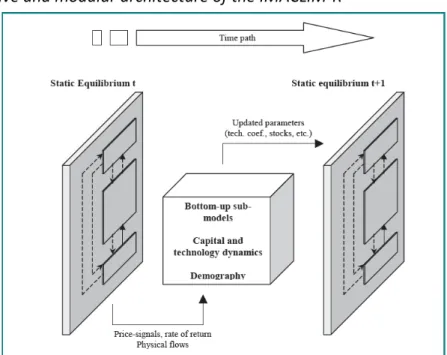
IMACLIM-R is a model of the world economy2 that covers the period 2001-2100 in yearly steps 22
through the recursive succession of annual static equilibria and dynamic modules (Figure 1). 23
15
The annual static equilibrium determines relative prices, wages, labour, value, physical flows, 1
capacity utilization, profit rates and savings at date t as a result of short term equilibrium 2
conditions between demand and supply on goods, capital and labor markets. The dynamic 3
modules are sector-specific reduced forms of technology-rich models, which take the static 4
equilibria at date t as an input, assess the reaction of technical systems to the economic 5
signals, and send new input-output coefficients back to the static model to compute the 6
equilibrium at t+1. Technical choices are flexible but, in a “putty-clay” representation 7
(Johansen, 1959), they modify only at the margin the input-output coefficients and labor 8
productivity embodied in the existing equipment that result from past technical choices to 9
represent the inertia in technical systems and the role of volatility in economic signals. 10
[Insert Figure 1 here] 11
The consistency of the iteration between the static equilibrium and dynamic modules relies 12
on ‘hybrid matrices’ (Hourcade et al., 2006), which ensure a description of the economy in 13
consistent money values and physical quantities (Sands et al., 2005). This dual description 14
represents the material and technical content of production processes and guarantees that 15
the projected economy is supported by a realistic technical background (informed by expert 16
views or sectoral analyses) and, conversely, that any projected technical system corresponds 17
to realistic economic flows and consistent sets of relative prices. In climate policy analysis, 18
this dual approach is crucial for energy goods to represent explicitly their carbon-to-energy 19
ratio (Malcolm and Truong, 1999). IMACLIM-R extends it to transportation as another key 20
sector of climate analysis by adopting an explicit representation of passenger and freight 21
mobility, expressed in passenger-km and ton-km respectively. 22
16
3.2 Modeling the dynamics of the transportation sector 1
This section enters more into the details of the representation of transport in the IMACLIM-R 2
model and sketches the way its major determinants are captured. 3
3.2.1 Passenger mobility demand
4
Households derive utility from the consumption of goods i above its minimum level, 5
(0)
i
C
−
C
i , and mobility servicesS
m :6
(
(0)) (
(0))
modes j i goods i whereC
.
1 i m j m i m bC
S
S
η η ξ ξ = =
−
−
∑
Π
m j S pkmU
(1) 7 8Here, the aggregate mobility service Sm is defined as a CES composite of pasengers.km in the
9
four modes under consideration (air, road, public3, and non-motorized) with the elasticity of 10
substitution between modes η and mode-specific parameters bj. The basic needs of mobility
11
(0) m
S
measures constrained mobility (ie the minimum level that households have to satisfy, 12essentially for commuting) and ξm is the elasticity of utility to the level of mobility service.
13
Households maximize utility under a twofold constraint that affects transportation decisions. 14
On the one hand, the standard budget constraint (2) captures that transport-related 15
expenditures enter into a tradeoff with the consumption of other goods Ci paid at price pi.
16
The mobility services provided by public and air transport modes are paid at their end-use 17
prices, ppublic and pair respectively, including fuel, O&M and capital costs. On the contrary,
18
private modes are auto-produced by households at an end-use price that only includes liquid 19
fuels (or electricity) costs (paid at prices pliquidand pelecrespectively), given aggregate unitary 20
17 consumption per unit of distance, cars
liquid
α and cars elec
α . Note that fixed costs associated to car 1
ownership do not enter into this tradeoff, but are considered in households investments. 2
The income constraint can then be written as 3
(
cars . cars.)
i i public public air air liquid liquid elec elec cars
i
Income=
∑
p C⋅ +p ⋅pkm +p ⋅pkm + α p +α p pkm (2) 45
On the other hand, the demand for transportation services by households and modal share 6
is constrained by a time budget constraint (3) to represent the stability of travel time budget 7
across time and space at a regional or national scale. This assumption is supported by 8
number of studies, which demonstrate that, at an aggregate and average level, households 9
allocate a fixed amount of time Tdisp to transportation, regardless of transportation costs.
10
(see Mokhtarian and Chen (2004) for an extended discussion), with rather close outcomes in 11
terms of travel time budgets: 1.1–1.3 h per traveler per day (Zahavi and Talvitie, 1980), 50 12
min to 1.1 h per person per day (Bieber et al., 1994), 1.1 h per person per day (Schafer 13
and Victor, 2000) or 1.3 h per person per day (Vilhelmson, 1999). The time constraint can 14
then be written as: 15 Modes j 0 ( ) j pkm disp j du T v u =
∑ ∫
(3) 16 17In equation (3), v uj
( )
measures the marginal speed of transportation mode j, that is the 18speed for one additional passenger-kilometer. This variable depends on congestion effect, as 19
measured by the utilization rate of transportation capacities for mode j, Captransportj : the
20
higher the utilization rate, the lower the effective “speed” of the mode (Figure 2). This 21
18
representation is an extrapolation, at a very aggregated level, of the “macroscopic 1
fundamental diagram” on the relations between vehicles fluxes, speed and infrastructure 2
capacity at the scale of a large transportation network (Geroliminis and Danganzo, 2008). 3
This curve is specific to each mode with, for example, very little (strong) effect for rail 4
passenger (road) transport4. 5
[Insert Figure 2 here] 6
This structure with a twofold constraint allows capturing number of stylized facts of 7
passenger transportation: 8
• the rebound effect of energy efficiency improvements on mobility: more efficient 9
transportation vehicles free up resources (via lower fuel expenditures), which allow 10
an increase consumption of all goods and services within budget constraint (2), 11
including higher mobility demand. 12
• the induction effect of infrastructure deployment on mobility demand: for a given 13
transportation mode, adding up infrastructure decreases the congestion constraint 14
but the marginal effect of infrastructure deployment depends on the shape of the 15
congestion curve (Figure 2). This makes passenger.kms in that mode less time-16
consuming and allows households to increase overall travel demand within their time 17
budget (3). 18
• the modal breakdown between different modes: the four modes (air, road, public, 19
and non-motorized) are explicitly differentiated according to their costs, mobility 20
service (measured by their speed) and the availability of infrastructure determining 21
congestion levels. Given these characterictics, effective modal breakdown then 22
results endogenously from a tradeoff within the twofold income constraint (2) and 23
19
time budget (3). Note that the time budget constraint implies an implicit value of 1
travel time, given by the Lagragian multiplier of the constraint in households’ 2
maximization program. 3
• the constraints imposed on mobility needs by firms’ and households’ location: this 4
concerns in particular the importance of daily travels that households have no choice 5
but to realize to satisfy specific travel purposes (essentially, commuting and shopping 6
travels. They are represented by the basic needs parameter (0) m
S
in equation (1). 78
3.2.2 Freight mobility demand
9
Production possibilities in all sectors are described using a Leontief function with fixed 10
intensity of labor, energy and other intermediary inputs in the short-term (but with a flexible 11
utilization rate of installed production capacities). This means in particular that, at a given 12
point in time, the intensity of production in each of the three freight transportation modes 13
(air, water and terrestrial transport) is measured by input-output coefficientsICF j, , which 14
define a linear dependence of freight mobility in a given mode j to production volumes. Note 15
that “terrestrial transport” includes both trucks and rail modes because of data limitations, 16
since the two modes correspond to a single aggregated sector in the economic accounting 17
matrixes used for Imaclim-R calibration, GTAP 6 (Dimaranan and McDougall, 2006). The 18
input-output coefficients capture implicitly (a) the spatial organization of the production 19
processes in terms of specialization/concentration of production units and (b) the 20
constraints imposed on distribution in terms of distance to the markets and just-in-time 21
processes, both driving the modal breakdown and the intensity of freight mobility needs. 22
The input-output coefficients evolve in time to capture changes in the energy efficiency of 23
20
freight vehicles, in the logistic organization of the production/distribution process and in the 1
modal breakdown. 2
3
3.2.3 Transportation technologies and energy efficiency
4
The motorization rate determines the access to the automobile mode among households’ 5
choices. In each region, it is related to per capita disposable income with a variable income-6
elasticity in function of income levels (Dargay et al, 2007): in regions with low income per 7
capita, the elasticity is maintained at a low level (0.3) because very poor people rely 8
essentially on non-motorized modes and public transport; at middle-income levels (from 9
$3,000 to $10,000 per capita), this elasticity is set at 2 to capture the acceleration of the 10
access to private motorized mobility (motorization grows twice as fast as income); finally, at 11
the highest levels of income comparable to those in the OECD, the elasticity decreases 12
progressively to represent equipment saturation and it is assumed, in particular, that the 13
motorization rate never exceeds the current US value (0.7 vehicle per person) 14
Energy efficiency in private vehicles is measured by the evolution of parameters cars liquid
α and 15
cars elec
α in equation (2), which result from households’ decisions on the purchase of new 16
vehicles among three types of technologies: standard vehicles (consuming only liquids), 17
hybrid cars (consuming both electricity and fuels) and “electric vehicles” (using only 18
electricity). The description of transport technologies remains at a rather aggregate level to 19
facilitate the dialogue with the top-down macroeconomic description: “electric vehicles” 20
represent implicitly all types of vehicles that use electricity as service provider, including fuel 21
cells and hydrogen vehicles. Technologies are differentiated by their unitary fuel 22
consumption and their capital costs (endogenously decreasing in function of the learning-by-23
21
doing process), and decisions among them are based on a mean cost minimization criterion 1
under imperfect expectations. 2
Energy efficiency for freight transportation is not represented through explicit vehicle 3
technologies but is captured implicitly through the evolution of the input-output coefficients 4
measuring, for each mode (water, air and terrestrial transport), the energy requirements for 5
the production of final transportation goods. These coefficients are responsive to energy 6
price variations to capture the incentive for technical progress in function of market 7
conditions (for example, the average fuel consumption of trucks evolves with a (-0.3) price-8
elasticity). 9
4 –Low carbon society and the transportation sector
104.1 Definition of the scenarios 11
To quantitatively assess the role of targeted policies for the transportation sector in the 12
transformation to low carbon societies, two sets of scenarios are compared. Both 13
correspond to the same climate objective, as captured by an identical emission trajectory 14
corresponding to a stabilization target of 440–485 ppm CO2: global CO2 emissions peak in 15
2017 and are decreased by 20% and 60% with respect of 2000 level in 2050 and 2100, 16
respectively (Barker et al. 2007, Table TS2).Each year, the model finds the level of carbon tax 17
that constrains emissions to the exogenous target given for that period, tax revenues are 18
recycled in a lump-sum manner within each region5.
19
The two sets of scenarios are distinguished by the nature of transport-related policies that 20
are introduced in parallel with the carbon tax. 21
22
In the first set of scenarios (S1), a continuation of current trends in terms of investment 1
choices driving mobility demand is assumed: 2
• Constrained mobility (measured by (0) m
S
in equation (1)) evolves proportionally to 3total mobility
S
m. This assumption is consistent with the constancy of the ratio of 4Commuting Distances over Total mobility (around 30%) in the United States over the 5
period 1969-2009 (NHTS, 2009). For the sake of simplicity, this assumption is 6
extended to all regions and this share is taken equal to 50% to account for all basic 7
mobility purposes (including commuting but also shopping, access to services). This 8
represents a proxy for a continuation of urban sprawl when households gain better 9
accessibility thanks to increased performance of transport modes. 10
• The allocation of investments in transportation infrastructure follows mobility 11
demand for each transportation mode. This means that investments are decided so 12
that the extensions of the infrastructure network associated to a given mode (roads, 13
railways, airports) follow the increase of passenger-km covered with this mode. This 14
is a proxy to represent that investment choices are mainly driven by the objective to 15
avoid congestion. 16
• The freight transport intensity of production remains constant ie the input coefficient 17
per unit of production remains at its baseline level. This means that the 18
production/distribution process keeps a similar organization throughout the period 19
and responds to transport cost increases (either due to energy or carbon prices) by 20
maintaining a constant dependence on transport instead of the increase observed in 21
recent years (McKinnon et al., 2010). 22
23
In the second set of run (S2), specific measures are implemented to control the ”behavior” 1
determinants of transportation in the course of the low-carbon transition. At this scale of 2
analysis, only very stylized representations are possible, they are “proxies” to encapsulate 3
rich policy packages implemented at different spatial scales; a detailed description of the 4
content of these policies can be found in (Santos et al., 2010) for passengers mobility and 5
(McKinnon et al., 2010) for freight transportation (the articles cited in the first paragraph of 6
section 2.2 also provide case studies of such policy packages). 7
We test here the effect of these measures at an aggregate level if they are able to trigger (i) 8
spatial reorganizations at the urban level and soft measures towards less mobility-9
dependent agglomerations, (ii) reallocation of investments in favor of public modes at 10
constant total amount for transportation infrastructure and (iii) adjustments of the logistics 11
organization to decrease the transport intensity of production/distribution processes and 12
optimize the use of vehicles (e.g., through improved backloading, more space efficient 13
packaging, more transport-efficient order cycles, etc.) in anticipation of very high long-term 14
transport costs. These measures affect three crucial determinants of transport activities that 15
are explicitly represented in IMACLIM: basic mobility (0) m
S
(equation (1)), transport capacities 16Captransportj (equation (3)) and ICF j, (section 2.2.2). 17
Given the absence of reliable and comprehensive data on the cost of implementation of 18
these measures, a redirection of investments at constant total amount is assumed and the 19
following simplifying assumptions are made: 20
• a progressive decoupling of basic mobility (0) m
S
with respect to total mobilityS
mfrom 2150% in 2020 to 40% in 2060 and after. 22
24
• a limitation of investments in road and air infrastructures causing a saturation of 1
transportation capacities Captransportroad and Captransportair and hence a maximum
2
threshold to mobility offered by these modes targeted at 7500km/capita and 3
2000km/capita respectively. These levels correspond approximately to current 4
mobility levels in Europe for road transport, and in North America for air transport. 5
Note that for regions (essentially North America) with mobility levels above the 6
threshold for road transport, a stagnation of transportation capacities are assumed. 7
• a 1% yearly decrease ofICF j, representing a decrease of the transport intensity of 8
production/distribution processes, and a 50% increase of the terrestrial freight 9
transportation energy efficiency reactivity to energy prices, representing the 10
optimization of vehicles use. 11
12
The modeling experiment then comprises: 13
- 48 BAU scenarios, corresponding to scenarios for which there is no constraint on CO2 14
emissions. 15
- 48 S1 stabilization scenarios, corresponding to stabilization scenarios with a “carbon 16
price only” strategy. 17
- 48 S2 stabilization scenarios, where “transportation policies” are implemented as 18
complementary measures to the carbon price. 19
These scenarios delineate the uncertainty on (i) Oil and Gas supply, (ii) coal supply, (iii) 20
substitutes to oil, (iv) technological change and technologies potentials and costs, (v) 21
lifestyles evolutions (see more details in (Waisman et al., 2012)). Here, we focus on the 22
transportation sector, and its interactions with the rest of the economy, to disentangle the 23
25
mechanisms at play in the alternative dynamics of passengers’ transportation (Section 4.2) 1
and freight transportation (Section 4.3), and analyze how the impacts of these alternative 2
dynamics impact the rest of the economy (Section 4.4). 3
4.2 Climate policy and Passenger transport 4
Even in stabilization scenarios, the emissions from passengers’ transport are increasing 5
during the first half of 21st century and remain above their 2010 level in 2100 for all 6
scenarios (Table 1). This means that, in stabilization scenarios where global emissions are 7
decreased by 60% compared to 2000, transport represents a dominant share of remaining 8
emissions at the end of the century (up to 70% in S1). Average emissions from passenger 9
transport are close in the two stabilization scenarios (4.8 GtCO2), but the upper bounds are 10
significantly higher in S1. This demonstrates the risk of high passenger transport emissions in 11
absence of complementary transport-specific measures if technology potential (especially on 12
electric vehicles) are limited. 13
[Insert Table 1 here] 14
To understand the dynamics of these emissions among the modes, the mechanisms are 15
decomposed into (i) global mobility evolution, (ii) modal structure evolution and (iii) vehicle 16
fleet efficiency improvement and/or electrification. 17
(i) The rapid increase of mobility in baseline scenarios is only moderately affected by 18
mitigation policies and, in S1 and S2 scenarios, global mobility in 2100 is only 13% and 19% 19
lower than in the baseline, respectively (Table 2). This weak effect is due to the lowering of 20
international oil prices (thanks to lower oil demand induced by the climate policy) limiting 21
the increase of fuel costs and to inertia in the transportation infrastructure, which become 22
active only in the second half of the century. 23
26
[Insert Table 2 here] 1
2
(ii) The modal structure is similar in the baseline case and in S1 scenarios, but very different 3
in the S2 scenarios with significant shift from personal vehicles to low carbon modes (public 4
transport and non-motorized) and a moderation of air transportation increase (Table 3) 5
[Insert Table 3 here] 6
(iii) Mean liquid fuel consumption of the personal vehicle fleet captures both the increased 7
efficiency of internal combustion engines (ICE) and the electrification of the fleet through 8
the diffusion of hybrid and electric vehicles (Figure 3). In S1 scenarios, the carbon price 9
ensures significantly better vehicle efficiency than in BAU scenarios (- 28% on average in 10
2100). This efficiency effect is slowed in S2 scenarios because carbon prices are lower and 11
the fleet turn-over is slower due to lower vehicle use, both effects affecting the diffusion of 12
efficient ICE and electrified vehicles. 13
[Insert Figure 3 here] 14
This analysis demonstrates very different determinants of emission reduction trends in the 15
transportation sector depending on the measures adopted. Under “carbon-price only” (S1 16
scenarios), the major effect is due the diffusion of energy efficiency in vehicles, whereas 17
modal shift and mobility reduction play a dominant role when appropriate transport policies 18
are implemented (S2 scenarios). 19
27 4.3 Climate policy and Freight transportation 1
Total emissions from freight transport are on average 24% and 48% lower than in the 2
baseline for S1 and S2 scenarios respectively, the difference being critically explained by the 3
freight transportation input per unit of production in S2 and S1 4
Under carbon price only policy (S1 scenarios), the reduction of emissions from inland freight 5
due to carbon pricing is slow and moderate even on the long-run (emissions are reduced by 6
25% in 2100) (Table 4). 7
[Insert Table 4 here] 8
Under constant freight transportation input per unit of production, freight transport 9
emissions reductions come from (i) a reduction of industrial production due to contraction of 10
activity and structural change towards less transport-intensive activities (e.g., services) 11
(Figure 4) and (ii) vehicle efficiency gains allowing a decoupling of transport activity and 12
emissions (Figure 5). In S2 scenarios, the “transportation policies” contribute additionally to 13
emission reduction by decreasing the freight transportation input per unit of production and 14
the unitary liquid fuels consumption from freight transportation vehicles. 15
[Insert Figure 4 here] 16
[Insert Figure 5 here] 17
Note that maritime and air freight transport emissions are only moderately affected by the 18
climate policy. In 2100, the 23% reduction with respect to BAU is essentially due to lower 19
freight mobility needs (20% ton.kilometers on average in 2100) in parallel with less overall 20
economic activity and less trade (because of higher international transport prices implied by 21
the carbon price). 22
28 1
4.4 The transportation sector in low carbon transitions: macroeconomic implications 2
This final section analyzes how the implementation of specific measures to control mobility 3
affects the rest of the economy in the transition to low-carbon futures. Note that we limit 4
our analysis to macroeconomic assessments in GDP terms, without taking into account the 5
costs and benefits of mitigation in the form of (avoided) climate damages and adaptation 6
costs. 7
First, the carbon intensity of liquid fuels is slightly lower in S2 scenarios. Indeed,the volume 8
of biofuels is very close in the two scenarios (because it is more driven by land competition 9
than by energy prices) and lower liquid fuel production in S2 scenarios means a higher share 10
of biofuels (34.9% on average in 2100 in S2 scenarios vs. 32.4% in S1 scenarios) 11
[Insert Table 5 here] 12
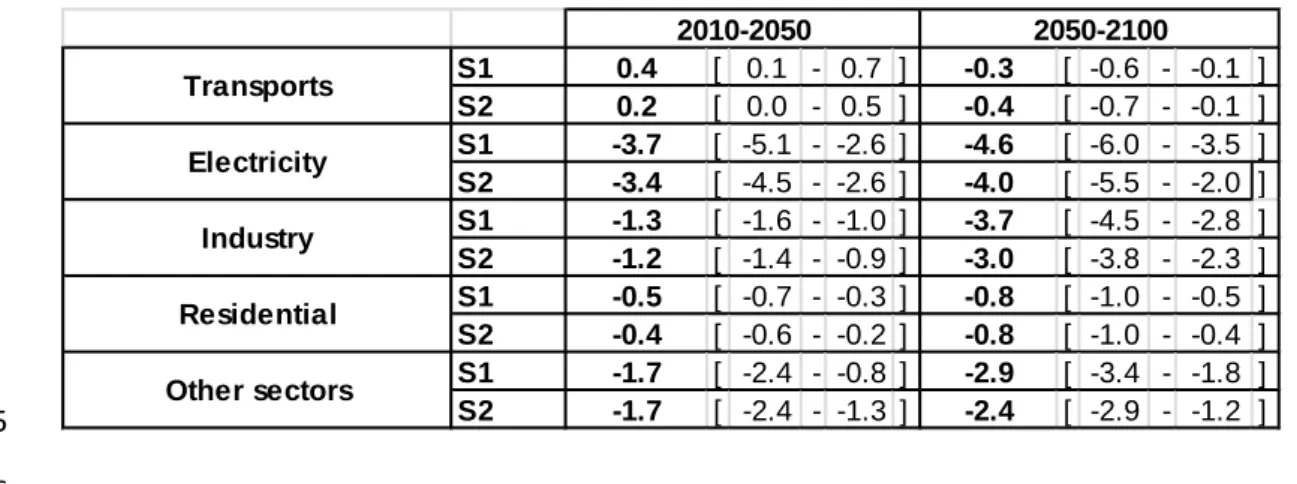
Second, the sectoral structure of emission reductions is significantly different under the two 13
groups of scenarios (Table 5). The decarbonization efforts bear mainly on non-transport 14
sectors (electricity, industry and residential) since transportation has the lowest 15
decarbonisation rate (its emissions even continue to rise despite stabilization policies over 16
2010-2050 before slightly declining in the end of the period). The “transportation policies” in 17
S2 allow increasing the contribution of the transportation sector to mitigation efforts (as 18
captured by lower values of emission variations for transport in Table 5) and other sectors 19
can then slow their decarbonization effort. This concerns essentially the power sector and, in 20
the long run, the industry. 21
29
As a consequence, the carbon price path necessary to respect the global emissions trajectory 1
objective is lower in S2 than in S1 (Figure 6), driving reductions of macroeconomic mitigation 2
costs. 3
[Insert Figure 6 here] 4
In S1, very high carbon price are necessary in the second part of the 21st century to reach the 5
450 ppm target via the proposed emission trajectory: in 2100, the average price across 6
scenarios reach almost 600 $/tCO2 with a risk of attaining 1200$/tCO2 under the most
7
pessimistic technological assumptions. Waisman et al. (2012) showed that this high carbon 8
price is associated with high macroeconomic losses reaching on average 4.6% of BAU GDP in 9
2100. The important long-term macroeconomic losses can be explained by (i) the inertia of 10
infrastructures, location choices, and urban forms embedded in the model, and (ii) by the 11
important rebound effect of mobility that requires very high carbon prices in the second half 12
of the century to meet stringent emissions targets. In other words, lack of change in 13
infrastructure and associated demand dominate the cost assessment in the long-run, since 14
all the sectors other than transportation have already made substantive cuts in their 15
emissions. 16
In S2, the higher decarbonization of the transportation sector allows carbon prices to be 17
lower: on average carbon prices are 40% lower in 2100 in S2 scenarios than in S1 scenarios 18
and in particular, prices above 600$/tCO2 at this time horizon are excluded. The associated 19
macroeconomic cost of stabilization is also significantly reduced: the long-term 20
macroeconomic cost of mitigation (GDP loss compared to baseline GDP) is 0.7% in S2 21
scenarios (to be compared with 4.6% on average in S1 scenarios); in 2100 global real GDP is 22
30
4.2% higher on average (ranging from 1.8% to 6.7% depending on the assumptions on fossil 1
fuels supply, technologies and lifestyles) in S2 scenarios than in S1 scenarios. 2
3
5. Conclusion
4This paper investigates the role (passenger and freight) transportation activities in the 5
transition to low carbon societies with a particular attention to specific measures designed 6
to control the growth of mobility. This is done by adopting a Energy-Economyc-Environment 7
model that represents explicitly the transport sector, including its non-price determinants 8
(urban organization, infrastructures, spatial organization), and captures its interactions with 9
the rest of the economy througha general equilibrium setting 10
Transport proves to be the sector for which carbon emissions are the more difficult to 11
reduce and hence represents a dominant share of remaining emissions in the long-term. 12
Because of its weak reactivity to energy price increases, very high levels of carbon price must 13
be imposed in the second half of the century to reach low mitigation targets: in 2100, the 14
average value of carbon prices is around 600$/tC02, with a risk of attaining 1200$/tCO2. 15
Controlling the growth of mobility would allow limiting these effects by offering mitigation 16
potentials independent of carbon prices. This study considers three potential sources of 17
mobility moderation: urban reorganizations lowering constrained mobility (i.e. mobility for 18
commuting and shopping), infrastructure deployment favoring low-carbon modes and 19
changes of logistics organization driving lower freight mobility intensity of 20
production/distribution. They allow excluding carbon prices above 600$/tCO2 and hence 21
help limiting macroeconomic cost of mitigation policies. 22
31
An important caveat for these conclusions is that they rely on an aggregated level of 1
description, which does not permit to represent explicitly the underlying policy measures 2
adopted at different scales to trigger these evolutions, like land planning, transport policies 3
per se or fiscal policies (e.g., Nivola, 1999). This means that we do not enter into the 4
discussions about the policy instruments to be combined, although this discussion is 5
particularly crucial for the transport sector, since the wide range of factors driving mobility 6
calls for fine adjustments of different policies. This means also that we ignore some 7
potentially important indirect effects of these policies beyond the transport sector, like 8
those affecting real estate markets, which may drive land price changes with a potentially 9
important effect on households’ purchase power and location decisions. 10
Despite these limitations, our results are robust enough to conclude that investigating 11
further the synergies between carbon price schemes and a wide set of spatial and housing 12
policies aimed at controlling mobility needs is a critical precondition to set in place efficient 13
energy policies, all the more so in case of ambitious climate mitigation strategies. Further 14
investigation of these questions—and with associated issues such as welfare and distribution 15
impacts— goes along with further development of the modeling approach to embark some 16
crucial effects, like the interplay between transport infrastructure, modal choice, real estate 17
markets and scarcity rents. 18
19 20 21
32 References
1
Åkerman, J., and M. Höjer. 2006. « How much transport can the climate stand?—Sweden on 2
a sustainable path in 2050 ». Energy policy 34 (14): 1944-1957. 3
Allcott, H, 2010, ’Beliefs and Consumer Choice’ , Working Paper MIT (December). 4
Allcott, H, Wozny, N., 2011,‘Gasoline Prices, Fuel Economy, and the Energy Paradox.’ 5
Working Paper MIT (July). 6
Allcott, H., 2011. ‘Consumers’ Perceptions and Misperceptions of Energy Costs.’, American 7
Economic Review, Papers and Proceedings, 101(3), 98-104. 8
Anable, J, Brand, C, Tran, M, Eyre, N, 2012, “Modelling transport energy demand: A socio-9
technical approach”, Energy Policy 41,125–138 10
Anable, Jillian, Sally Cairns, Lynn Sloman, Phil Goodwin, Alistair Kirkbride, and Carey Newson. 11
2005. « ’Soft’ Measures – soft option or smarter choice for early energy savings in the 12
transport sector? » 671-685. 13
Anderson, S., Kellogg, R, Sallee, J., 2011, What Do Consumers Believe About Future Gasoline 14
Prices?, NBER Working Paper No. w16974 15
Banister, David. 2000. European Transport Policy and Sustainable Mobility. Taylor & Francis. 16
Barkenbus, J, 2010.’ Eco-driving: An overlooked climate change initiative’, Energy Policy 38 17
(2), 762–769 18
Barker T, Bashmakov I, Bernstein L, Bogner JE, Bosch PR, Dave R, Davidson OR, Fisher BS, 19
Gupta S, Halsnæs K, Heij GJ, Kahn Ribeiro S, Kobayashi S, Levine MD, Martino DL, 20
Masera O, Metz B, Meyer LA, Nabuurs G-J, Najam A, Nakicenovic N, Rogner HH, Roy J, 21
Sathaye J, Schock R, Shukla P, Sims REH, Smith P, Tirpak DA, Urge-Vorsatz D, Zhou D 22
(2007): Technical Summary. In: Climate Change 2007: Mitigation. Contribution of 23
Working Group III to the Fourth Assessment Report of the Intergovernmental Panel on 24
Climate Change [B. Metz, O. R. Davidson, P. R. Bosch, R. Dave, L. A. Meyer (eds)], 25
Cambridge University Press, Cambridge, United Kingdom and New York, NY, USA. 26
Bento, A. M., M. L. Cropper, A. M. Mobarak, and K. Vinha. 2005. « The effects of urban 27
spatial structure on travel demand in the United States ». Review of Economics and 28
Statistics 87 (3): 466-478. 29
Bieber, A., Massot, M.-H., Orfeuil, J.-P., 1994. ‘Prospects for daily urban mobility’. Transport 30
Reviews 14 (4), 321–339. 31
Bristow, Abigail L., Miles Tight, Alison Pridmore, and Anthony D. May. 2008. « Developing 32
pathways to low carbon land-based passenger transport in Great Britain by 2050 ». 33
Energy Policy 36 (9) (septembre): 3427-3435. doi:10.1016/j.enpol.2008.04.029. 34
Brand, C, Tran, M, Anable, J, 2012, The UK transport carbon model: An integrated life cycle 35
approach to explore low carbon futures Energy Policy 41, 107–124 36
Brueckner, J. K. 2000. « Urban sprawl: Diagnosis and remedies ». International regional 37
science review 23 (2): 160-171. 38
Cairns, S., L. Sloman, C. Newson, J. Anable, A. Kirkbride, and P. Goodwin. 2004. « Smarter 39
choices-changing the way we travel ». 40
33
Cairns, S., L. Sloman, C. Newson, J. Anable, A. Kirkbride, and P. Goodwin. 2008. « Smarter 1
choices: assessing the potential to achieve traffic reduction using ‘soft measures’ ». 2
Transport Reviews 28 (5): 593-618. 3
Chapman, L. 2007. « Transport and climate change: a review ». Journal of transport 4
geography 15 (5): 354-367. 5
Chum H, Faaij A, Moreira J, Berndes G, Dhamija P, Dong H, Gabrielle B, Goss Eng A, Lucht W, 6
Mapako M, Masera Cerutti O, McIntyre T, Minowa T and Pingoud K (2011). Bioenergy. 7
In: O. Edenhofer, R. Pichs-Madruga, Y. Sokona, K. Seyboth, P. Matschoss, S. Kadner,, T. 8
Zwickel, P. Eickemeier, G. Hansen, S. Schlömer, C. von Stechow (eds) IPCC Special 9
Report on Renewable Energy Sources and Climate Change Mitigation , Cambridge 10
University Press, Cambridge, United Kingdom and New York, NY, USA. 11
Dahl, C, 2012,‘Measuring global gasoline and diesel price and income elasticities’ ,Energy 12
Policy, 41, 2-13 13
Dargay, J., Gately, D., Sommer, M., 2007, ‘Vehicle ownership and income growth, worldwide: 14
1960–2030’, Energy Journal, 28, 143–170 15
Dimaranan, B., and R. A. McDougall. 2006. Global Trade, Assistance and Production: The 16
GTAP 6 Data Base, Center for Global Trade Analysis. Purdue University, West Lafayette, 17
IN. 18
Geroliminis, N., and C. F. Daganzo. 2008. « Existence of urban-scale macroscopic 19
fundamental diagrams: Some experimental findings ». Transportation Research Part B: 20
Methodological 42 (9): 759-770. 21
Glaeser, Edward L., and Matthew E. Kahn. 2010. « The greenness of cities: Carbon dioxide 22
emissions and urban development ». Journal of Urban Economics 67 (3) (mai): 404-23
418. doi:10.1016/j.jue.2009.11.006. 24
Goodwin, P, Dargay, J, Hanly, M,2004, ‘Elasticities of Road Traffic and Fuel Consumption with 25
Respect to Price and Income: A Review’.Transport Reviews 24 (3), 275-292. 26
Goodwin, P. B. 1996. « Empirical evidence on induced traffic ». Transportation 23 (1): 35-54. 27
Grazi, Fabio, Jeroen C.J.M. van den Bergh, and Jos N. van Ommeren. 2008. « An Empirical 28
Analysis of Urban Form, Transport, and Global Warming ». The Energy Journal 29 (4) 29
(octobre 1). doi:10.5547/ISSN0195-6574-EJ-Vol29-No4-5. 30
http://www.iaee.org/en/publications/ejarticle.aspx?id=2279. 31
Greene, D, 1998, ‘Why CAFE worked?’,Energy Policy,26(8), 595–613 32
Greene, D. L., S. E. Plotkin, and Pew Center on Global Climate Change. 2011. Reducing 33
greenhouse gas emissions from US transportation. Pew Center on Global Climate 34
Change Washington, DC. 35
Greening, L, Greene, D , Difiglio, C ,2000,‘Energy efficiency and consumption – the rebound 36
effect – a survey’,Energy Policy, 28(6), 389-401. 37
Hickman, R., O. Ashiru, and D. Banister. 2011. « Transitions to low carbon transport futures: 38
strategic conversations from London and Delhi ». Journal of Transport Geography. 39
34
Hickman, Robin, Olu Ashiru, and David Banister. 2010. « Transport and climate change: 1
Simulating the options for carbon reduction in London ». Transport Policy 17 (2) 2
(mars): 110-125. doi:10.1016/j.tranpol.2009.12.002. 3
Holden, E., and I. T. Norland. 2005. « Three challenges for the compact city as a sustainable 4
urban form: household consumption of energy and transport in eight residential areas 5
in the greater Oslo region ». Urban Studies 42 (12): 2145. 6
Hourcade, JC, Jaccard, M, Bataille, C et Ghersi, F, 2006, ‘Hybrid Modeling : New Answers to 7
Old 8
Hourcade, J-C., 1993, ‘Modelling long-run scenarios. Methodology lessons from a 9
prospective study on a low CO2 intensive country’, Energy Policy, 21(3), 309-326. 10
Hymel, K. M., K. A. Small, and K. V. Dender. 2010. « Induced demand and rebound effects in 11
road transport ». Transportation Research Part B: Methodological 44 (10): 1220-1241. 12
IEA, 2011a, CO2 Emissions from Fuel Combustion, OECD, Paris. 13
IEA, 2011b, World Energy Outlook 2011 , OECD,Paris. 14
International Energy Agency. 2009. « Transport, Energy and CO2: Moving Toward 15
Sustainability ». OECD/IEA. 16
International Transport Forum, 2007. Workshop on ecodriving: findings and messages for 17
policy makers, November 22–23. Available at: 18
http://www.internationaltransportforum.org/Proceedings/ecodriving/EcoConclus.pdf 19
IPCC (2007). Summary for Policymakers. In: B. Metz, O.R. Davidson, P.R. Bosch, R. Dave, L.A. 20
Meyer (eds) , 21
Johansen L., 1959, “Substitution versus Fixed Production Coefficients in the Theory of 22
Growth: A synthesis”, Econometrica, 27, 157-176. 23
Johansson, Bengt. 2009. « Will restrictions on CO2 emissions require reductions in transport 24
demand? » Energy Policy 37 (8) (août): 3212-3220. doi:10.1016/j.enpol.2009.04.013. 25
Le Néchet, Florent. 2011. « Consommation d’énergie and mobilité quotidienne selon la 26
configuration des densités dans 34 villes européennes. » Cybergeo : European Journal 27
of Geography (mai 18). doi:10.4000/cybergeo.23634. 28
http://cybergeo.revues.org/23634. 29
Malcolm,G, Truong, P, 1999,‘The Process of Incorporating Energy Data into GTAP’, Draft 30
GTAP 31
McCollum, David, and Christopher Yang. 2009. « Achieving deep reductions in US transport 32
greenhouse gas emissions: Scenario analysis and policy implications ». Energy Policy 37 33
(12) (décembre): 5580-5596. doi:10.1016/j.enpol.2009.08.038. 34
McKinnon, Alan. 2010. Green Logistics: Improving the Environmental Sustainability of 35
Logistics. Kogan Page Publishers. 36
Metz, D. 2008. « The myth of travel time saving ». Transport Reviews 28 (3): 321-336. 37
Mindali, Orit, Adi Raveh, and Ilan Salomon. 2004. « Urban density and energy consumption: 38
a new look at old statistics ». Transportation Research Part A: Policy and Practice 38 (2) 39
(février): 143-162. doi:10.1016/j.tra.2003.10.004. 40