HAL Id: hal-01016399
https://hal.archives-ouvertes.fr/hal-01016399
Preprint submitted on 30 Jun 2014
HAL is a multi-disciplinary open access
archive for the deposit and dissemination of
sci-entific research documents, whether they are
pub-lished or not. The documents may come from
teaching and research institutions in France or
L’archive ouverte pluridisciplinaire HAL, est
destinée au dépôt et à la diffusion de documents
scientifiques de niveau recherche, publiés ou non,
émanant des établissements d’enseignement et de
recherche français ou étrangers, des laboratoires
Sensitivity analysis of an energy-economy model of the
residential building sector
Frédéric Branger, Louis-Gaëtan Giraudet, Céline Guivarch, Philippe Quirion
To cite this version:
Frédéric Branger, Louis-Gaëtan Giraudet, Céline Guivarch, Philippe Quirion. Sensitivity analysis of
an energy-economy model of the residential building sector. 2014. �hal-01016399�
Sensitivity analysis of an energy-economy model of the
residential building sector
Frédéric Brangera,b,1,∗, Louis-Gaëtan Giraudeta, Céline Guivarcha, Philippe
Quiriona,c
aCIRED, 45 bis, avenue de la Belle Gabrielle, 94736 Nogent-sur-Marne Cedex, France b
AgroParistech ENGREF, 19 avenue du Maine 75732 Paris Cédex c
CNRS
Abstract
In this paper, we discuss the results of a sensitivity analysis of Res-IRF, an energy-economy model of the demand for space heating in French dwellings. Res-IRF has been developed for the purpose of increasing behavioral detail in the modeling of energy demand. The different drivers of energy demand, namely the extensive margin of energy efficiency investment, the intensive one and build-ing occupants’ behavior are disaggregated and determined endogenously. The model also represents the established barriers to the diffusion of energy effi-ciency: heterogeneity of consumer preferences, landlord-tenant split incentives and slow diffusion of information. The relevance of these modeling assumptions is assessed through the Morris method of sensitivity analysis, which allows for the exploration of uncertainty over the whole input space. We find that the Res-IRF model is most sensitive to energy prices. It is also found to be quite sensitive to the factors parameterizing the different drivers of energy demand. In contrast, inputs mimicking barriers to energy efficiency have been found to have little influence. These conclusions build confidence in the accuracy of the model and highlight occupants’ behavior as a priority area for future empirical research.
1. Introduction
Numerical energy-economy models used for energy and climate policy as-sessment carry considerable uncertainty. First, just like any other model, they are incomplete representations of a real-world system. This indeterminacy gen-erates irreducible uncertainty. More specifically, the energy-economy systems they represent involve human behavior, the laws of which cannot be established
∗Corresponding author
Email addresses: branger@centre-cired.fr(Frédéric Branger),
giraudet@centre-cired.fr(Louis-Gaëtan Giraudet), guivarch@centre-cired.fr (Céline Guivarch), quirion@centre-cired.fr (Philippe Quirion)
with the same robustness as in natural sciences. Uncertainty increases fur-ther if one considers that energy-economy models are forward-looking tools for decision-making. As such, they are subject to future states of the world, which are unknown by nature.
Such deep, polymorphic uncertainty emphasizes the need to submit energy-economy models to sensitivity analysis. Though essential for transparency, sen-sitivity analysis can be a daunting task when models are based on non-linear relationships and involve large numbers of parameters, which is an important characteristic of energy-economy models. This difficulty is reflected by the domi-nant use of the “One-At-a-Time” (OAT) method of sensitivity analysis, in which model parameters are varied locally one after the other but never together at the same time. This technique does not allow modelers to explore the full space of uncertainty nor interactions between model inputs.
The heterogeneity of energy demand in buildings epitomizes the uncertainty associated with energy-system modelling and thereby the difficulty of sensitivity analysis. Building energy demand involves the use of a variety of technologies (e.g., heating, ventilation and air-conditioning systems, insulation techniques), a building stock that is heterogeneous in terms of its architecture and surrounding climate, and building users whose characteristics vary with respect to their ten-ancy status, preferences or income. Representing such a disaggregated system expands the sources of uncertainty in the associated models. Individual occu-pant behaviors, which are to a large extent unobservable, can only be mimicked by tentative functional forms, parameterized with incomplete data. Yet the multiplicity of technologies and agents imposes a large number of parameters. This context reinforces the so-called curse of dimensionality that hampers sen-sitivity analysis (Bellmann, 1957). Accordingly, sensen-sitivity analysis is typically rare in energy-economy models of the building sector (Mundaca et al., 2010; Kavgic et al., 2010). This is unfortunate: reducing energy demand in buildings is considered by scientists of the IPCC (Levine et al., 2007) and many policy-makers as the most cost-effective option to mitigate climate change; therefore substantiating this claim and designing practical ways to address it calls for reliable models.
In this paper, we assess an innovative model of building energy demand, Res-IRF, using a sensitivity analysis technique, the Morris method, that is ap-propriate for the degree of complexity of the model.
Res-IRF has been developed at CIRED to assess the long-term impact of energy efficiency policies on energy demand for space heating in French house-holds (Giraudet et al., 2012, 2011a). One prerequisite for such an assessment is to have a model that takes into account the complexity of energy-related de-cisions, an ability existing models of energy demand typically lack (Mundaca et al., 2010; Kavgic et al., 2010). Accordingly, the purpose with the develop-ment of Res-IRF was to improve decision criteria for technical and behavioral change. This materializes through the endogeneization of each of the different drivers of energy use: the intensive margin of energy efficiency investment (at
what level to invest?), the extensive one (whether or not to invest?) and
of some barriers to energy efficiency, such as heterogeneity in consumer prefer-ences, landlord-tenant split incentives and slow diffusion of information. Up to now, its operation had been assessed through preliminary OAT sensitivity anal-ysis and comparison with other models (see AppendixA), but never submitted to in-depth sensitivity analysis.
The Morris method of sensitivity analysis, also known as the Elementary Effects method, has been introduced by Morris (1991) and developed in partic-ular by Campolongo et al. (2007). It can be seen as a randomized OAT design. For each input, elementary effects are computed from different points in the input space. The mean and standard deviation of the elementary effects give a measure of importance of the input and its interactions with other inputs. This method reconciles the low computational cost of OAT techniques with the global focus of more advanced variance-based methods like the Sobol method (Saltelli et al., 2008). Application of the Morris method is growing in various fields of science; yet to our knowledge, in the energy-economy field, it has only been applied to the IMAGE model (Potting et al., 2002; Campolongo and Braddock, 1999).
The sensitivity analysis reported here went as follows. Preliminary Monte Carlo simulations revealed that Res-IRF’s main output, the energy use for space heating in French households in 2050, varied around the reference scenario by 25% at the 95% confidence level. Subsequent application of the Morris method revealed that this variability was due for the most part to future energy prices, which are exogenous to the model. The model is also quite sensitive to the factors parameterizing the different drivers of energy demand; in contrast, in-puts mimicking barriers to energy efficiency are less important. Less than 3% of the simulations crashed, which builds confidence in the stability of the model. Interactions between inputs did not prove important, so more advanced sensi-tivity analysis was not necessary. Even though the exercise did not eliminate all sources of uncertainty, it confirmed for us that the Res-IRF model manages to improve behavioral detail. As such, it provides reliable, intuitive predictions of the effect of energy price on energy demand. Lastly, the analysis highlights the need to systematically present several energy price scenarios, to better un-derstand the nature of the barriers to energy efficiency and to collect more data about building retrofits and occupants’ behavior.
Section 2 of this paper presents the Res-IRF model, stressing its innovative aspects as well as the uncertainty they create. Section 3 details the approach for the sensitivity analysis. Section 4 presents the results. Section 5 interprets the results and discusses the reliability of the model. Section 6 concludes.
2. An overview of the Res-IRF model
Res-IRF1 is a bottom-up simulation model of energy demand in the
resi-dential sector. It is calibrated against year 2008 data and run recursively in annual time steps. In the model, energy efficiency improvements materialize through the construction of new buildings and the retrofitting of existing ones. The model is finely detailed with technological and microeconomic representa-tions. As such, it can be seen as a hybrid energy-economy model (Hourcade et al., 2006). The models to which Res-IRF is most similar to are CIMS, the Canadian Integrated Modeling System (Jaccard and Dennis, 2006; Mau et al., 2008) and the residential module of NEMS, the U.S. National Energy Model-ing System (Wilkerson et al., 2013). A comprehensive description of the guidModel-ing principles, structure and input data needs of the Res-IRF model can be found in Giraudet et al. (2012). AppendixB of the present paper updates that description with some recent model developments.
2.1. Motivation
Before describing Res-IRF, it is worth mentioning the context in which it was developed. At a fundamental level, energy demand for heating in existing buildings can be decomposed into three drivers: the extensive margin of energy efficiency investment (how many dwellings are retrofitted); the intensive one (how energy efficient are these retrofits); and building occupants’ behavior (how
do occupiers set their heating thermostat?). State-of-the-art energy-economy
models typically endogenize the intensive margin of energy efficiency investment, keep the extensive one exogenous and hold occupants’ behavior constant.
A specific challenge to the modeling of energy demand is the representation of the alleged barriers to energy efficiency. Since the pioneering contribution of Jaffe and Stavins (1994) on the “energy efficiency gap”, a large body of litera-ture in economic and social sciences has been looking at barriers that misalign private investment in energy efficiency with its socially optimal level. These barriers include landlord-tenant split incentives and information spillovers. The most recent reviews of the literature on this subject conclude that neither the empirical existence of the barriers to energy efficiency nor their theoretical im-plications are well established (Gillingham et al., 2009; Allcott and Greenstone, 2012). This lack of knowledge is reflected in a perfunctory representation of the barriers in energy-economy models, which typically represent them collectively with abnormally high discount rate values2.
1
“Res-IRF” stands for the “Residential module of IMACLIM-R France”. IMACLIM-R France is a recursive general equilibrium model of the French economy developed at CIRED (Bibas et al., 2012). Linking Res-IRF and IMACLIM-R France allows for the clearing of energy markets and energy prices to be determined endogenously. This process is described in Giraudet et al. (2011a). In the present paper, Res-IRF is run with no link to IMACLIM-R France.
2
“Abnormal” here means any value higher than 7%, which is the value recommended by the U.S. Office of Management and Budget for private cost-benefit assessment (OMB, 2013)
Against this background, Res-IRF introduces two modeling innovations. First, it offers greater detail than just using high discount rates in the rep-resentation of the barriers to energy efficiency. Second, it endogenizes all three drivers of energy use in existing buildings. Linking investment and capital uti-lization allows model users to assess the rebound effect, that is, increases in energy service consumption in response to energy efficiency investment. This issue receives much attention in policy discussions. Furthermore, policy-makers in some countries have defined annual retrofitting targets. Endogenizing the volume of retrofits in Res-IRF allows model users to assess the contribution of policy instruments to meeting such targets. These modelling innovations how-ever lead to the creation of new sources of uncertainty, as the next subsections describe.
2.2. Driving forces
At the aggregate level, energy demand is determined as the product of an extensive output, the building stock, measured in square meters, and an intensive output, the specific energy use of the building stock, measured in
kW h/m2/year. Model outcomes are fully determined by three exogenous input
trajectories: population growth, GDP growth and energy prices. GDP growth determines the growth in floor area per capita, according to an elasticity; this, combined with population growth, determines the annual construction of new floor area. The floor area of existing buildings remains constant, except for some demolitions that occur at a constant annual rate. Energy prices drive energy efficiency improvements in both new and existing dwellings.
2.3. Technological detail
Res-IRF focuses on the use of electricity, natural gas, fuel oil and fuel wood for space heating. The building stock comprises single-family dwellings, multi-family dwellings and social housing. The technical characteristics of building envelopes and heating systems are not represented explicitly. Rather, the energy performance of existing buildings takes one of seven discrete values, covering la-bel G (the least efficient) to lala-bel A (the most efficient) of the French Energy Performance Certificate. Energy efficiency improvements are realized through transitions to higher energy labels and through fuel switches. The performance of new buildings takes one of three discrete values, corresponding to the min-imum requirements of the French building codes of 2005, 2012 and 2020 (as currently anticipated for the latter). The heating energy carrier and efficiency level of new constructed buildings are chosen simultaneously.
Representing energy efficiency improvements through energy label transi-tions facilitates the simulation of microeconomic decisions as discrete choices. It however also creates parametric and empirical uncertainty. As a given tran-sition could in reality be realized through different combinations of building envelope and heating system measures, its cost is hard to specify and likely to be dispersed over a range of possible values.
2.4. Microeconomic detail
Homeowners use discrete choice functions on the intensive margin of en-ergy efficiency investment. Logit functions allocate market shares across the seven different energy labels according to their respective life-cycle costs. A heterogeneity parameter controls for the spread in market share allocation. The life-cycle cost of each energy label is given by the sum of investment costs and discounted energy operating costs specific to this label. Investment costs de-cline with cumulative investment through learning-by-doing. The computation of life-cycle energy operating costs assumes myopic expectations of energy prices. Res-IRF adds several innovative features to this otherwise standard modeling framework. First, unlike most other models, in which abnormally high discount rates are used to represent all barriers to energy efficiency, the Res-IRF model considers discount rates with split incentives only. Owner-occupiers are assumed to have normal discount rates; homeowners who rent out their dwelling are assumed to have a higher than normal discount rate. Likewise, owner-occupiers of multi-family dwellings, who are not the sole decision-maker when it comes to the renovation of the whole building are assumed to discount the future more sharply than owner-occupiers of single-family dwellings. Second, the life-cycle costs of each energy label factor-in some intangible costs, which are calibrated so as to allow logit functions to replicate the energy label choices observed in 2008. As such, intangible costs can be interpreted as including all possible barriers to energy efficiency other than landlord-tenant split incentives. The impact of barriers is assumed to decrease over time with cumulative investment as a consequence of information spillovers. The introduction of intangible costs in the model and the mechanism by which they decrease come from the CIMS model (Jaccard and Dennis, 2006; Mau et al., 2008)3.
The extensive margin of investment corresponds to annual constructions of new buildings and annual retrofits of existing buildings. While the former derives directly from exogenous inputs in the model, the latter is determined endogenously. For a representative homeowner-dwelling bundle, a logistic func-tion is used to deduce the retrofitting rate from the average net present value of retrofitting. The average net present value is calculated as the difference between the average life-cycle cost of upgrading the dwelling and the life-cycle cost of staying in its current energy label. Beforehand, the average life-cycle cost (including intangible costs) of a retrofitting project is weighted by the mar-ket share of each possible energy label transition, determined by logit functions, as described above. This simulation framework is equivalent to assuming that homeowners have a heterogeneous taste for the utility derived from energy ser-vices (e.g., some are more sensitive to the cold than others) and that this hetero-geneity is normally distributed across the population. In this view, the logistic curve mimics the cumulative distribution function of the taste parameter.
Lastly, in both new and existing buildings, the utilization of newly installed
3
As discount rates in CIMS are not used to mimic split incentives only, intangible costs cannot be interpreted as representing the same barriers in the two models.
capital adjusts after investment. The underlying idea is that dwelling occupants optimize the consumption of energy services, in the case of this work the heating temperature. Improvements in the energy efficiency of the dwelling typically decrease the marginal cost of heating, hence increasing the quantity of heating consumed, a phenomenon known as the rebound effect. This is represented in Res-IRF as an iso-elastic response of the demand for energy service, measured as the ratio between effective energy use and the conventional one disclosed by the energy label, to the energy efficiency of the dwelling, measured as the conventional energy expenditure, that is, the conventional use disclosed by the label valued at current energy prices (see AppendixB for further detail).
3. Sensitivity analysis approach of Res-IRF
First, we perform Monte Carlo simulations to quantify overall uncertainty in the model. Second, we use the Morris method to identify the main sources of uncertainty. A preliminary step for both exercises is to assign probability distributions to the inputs of the model. These three steps are described in more detail below.
3.1. Variables of interest
In this work, we focus on uncertainty in total primary energy use, the main output of interest of the model. We compare it to its value in a reference scenario4 at two points in time, 2020 and 2050. Separating short- and
long-term effects is important for inputs like the learning rate, which parameterizes a dynamic process. As such the learning rate may be more influential in the long-term than in the short-term.
We use the term input to name any factor that is given a numerical value in the model. Model inputs fall into three categories:
• Exogenous input trajectories (EI) representing future states of the world: energy prices, population growth and GDP growth.
• Calibration targets (CT), which are empirical values the model aims to replicate for the reference year 2008. They include hard-to-measure ag-gregates such as the reference retrofitting rate and the reference energy label transitions.
• All other model parameters (MP), which reflect current knowledge on behavioral factors (discount rates, information spillover rates, etc.) and technological factors (investment costs, learning rates, etc.)
4
As the motivation of the work is to assess the fitness of the model for the purpose of increasing behavioral detail, we do not assess uncertainty around policy scenarios. Still, estimates of the sensitivity of the model to energy prices give insights into its sensitivity to energy taxes. Likewise, sensitivity to variation in investment costs gives insights into sensitivity to different levels of subsidies.
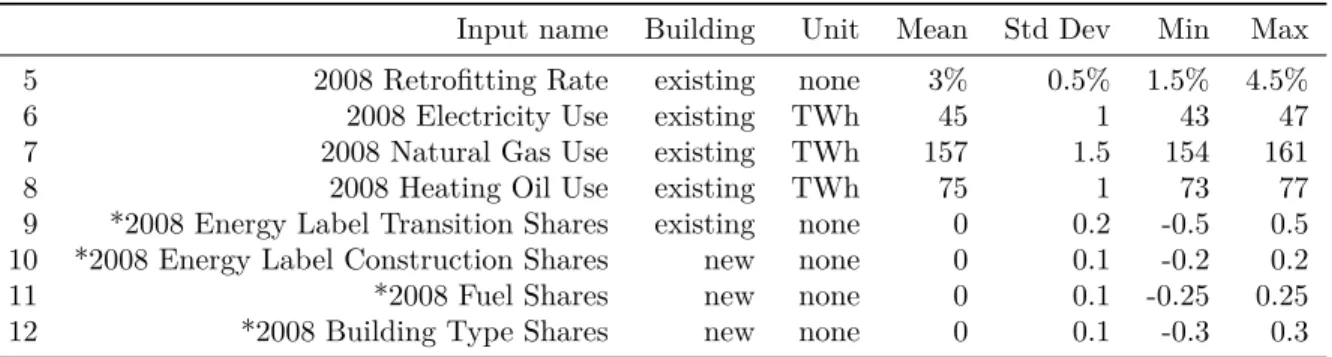
For each model input in the sensitivity analysis, we make specific assump-tions about the mean (which is the value used in the reference scenario), the probability distribution function and the range of values explored. Some factors cannot be manipulated as a simple scalar input and they are assessed through indirect inputs, as detailed in AppendixC. AppendixD provides a complete description of the 71 model inputs, by input type.
3.2. Monte Carlo simulations
1,500 Monte Carlo simulations are run. In each simulation, each input value is drawn pseudo-randomly from its probability distribution function. We use Latin Hypercube Sampling (McKay et al. 1979) to efficiently cover the input space. The probability density function of each input is divided into 1,500 regions of equal density. The sampling procedure then ensures that draws occur once in each region. Inputs are drawn from a uniform distribution within each region.
The number of simulations is large enough for us to compute the mean and standard deviation of the output distribution generated, hence get an aggregate view of the magnitude of uncertainty in the model. It is however not large enough for us to compute statistically significant standard regression coefficients (used to rank inputs by importance), so this motivates the use of the Morris method in a second step.
3.3. The Morris method
Sensitivity analyses are generally divided into local and global approaches (Confalonieri et al., 2010). Local sensitivity analyses, also known as “One At a Time” (OAT) techniques, are based on the estimation of partial derivatives (Campolongo et al., 2011). Partial derivatives are only informative at a global scale if some linearity and additivity conditions are met, which is rarely the case in energy-economy models (Saltelli and Annoni, 2010). In contrast, global sensitivity analyses evaluate the effect of a factor while all others vary as well. This allows modelers to efficiently explore the multidimensional input space. The global approach includes screening methods (mainly the Morris method), regression-based methods (computation of standard regression coefficients) and variance-based methods (mainly the Sobol method (Sobol, 1993)).
The Morris method can be thought of as an enhancement on the “perfunc-tory” OAT method (Morris, 1991; Saltelli and Annoni, 2010). It was developed in 1991 by Morris and went through some refinements with Campolongo et al. (2000) and Ruano et al. (2012). It is increasingly used5, for applications in
hydrology (Braddock and Schreider, 2006; Matthews et al., 2006), chemistry (Campolongo et al., 2007), agronomy (Richter et al., 2010), biophysics (Cool-ing et al., 2007), build(Cool-ing thermal simulation (Garcia Sanchez et al., 2014) and energy-economy modeling (Campolongo and Braddock, 1999).
5
The number of citations of Morris’ original paper in Thomson-ISI Web of Knowledge has grown steadily from below 10 per year until 2003 to more than 100 in 2013.
The Morris method can be summarized as follows. Consider a model with k random input variables Y = f(X1, ...Xk). Each model input (Xi)i∈{1,...,k}varies
across a uniform distribution in [0, 1]6. In the Morris method, each input varies
across p selected levels. The region of experimentation is then a k-dimensional
p-level grid. An elementary effect for variable i is defined by:
EEi(X1, ..., Xk, △) =
f (X1, .., Xi± ∆, ..Xk) − f(X1, ..., Xk)
±△
p is chosen to be even and △ equals p/(2(p − 1)) for symmetry
considera-tions. For each input variable, there are p/2 possible values below 0.5 and p/2 corresponding values (+△) above 0.5. This configuration leads to pk/2
differ-ent elemdiffer-entary effects per input7. The finite distribution of elementary effects
corresponding to the i-th input factor is called Fi. Then Gi is the equivalent
distribution of absolute values of elementary effects.
The sensitivity measures proposed by Morris are the estimated mean µ and standard deviation σ of Fi (Morris, 1991). Campolongo et al. (2011) propose a
third measure, µ∗, the estimated mean of G
i. Any significant difference between µ and µ∗ indicates a non-monotonic influence of the underlying input on the output.
Estimating µ∗, µ and σ requires sampling elementary effects from both F
i
and Gi. One efficient random sampling strategy is to build r trajectories of
(k + 1) points. As each trajectory gives k elementary effects, the computational cost of the experiment is r(k + 1). The construction of the trajectories requires several steps of randomization which are detailed in Morris (1991).
A decisive advantage of the Morris method is that it is “computationally cheap”. Around 50 simulations per input are needed, while the Monte Carlo re-gression requires 1,000 and the Sobol method 10,000 (Iooss, 2011). Nonetheless, the measure of importance µ∗compares favorably with those used in
variance-based methods to rank inputs according to their influence (Campolongo et al., 2007; Tang et al., 2007; Confalonieri et al., 2010). Furthermore, the Morris method allows one to handle unstable models that may crash when inputs are too different from their reference value. Unlike the Sobol method, it is possible to drop an elementary effect calculation without affecting the full design.
Ex ante, the Morris method seemed well-suited to the size and non-linear
nature of Res-IRF. We set the number of trajectories at r = 80, which, when applied to 71 inputs, led to 80×(71+1) = 5, 760 simulations. The computational cost incurred was low8. Ex post, the Morris method proved appropriate: Results
6
The normalized inputs are then converted from the original hypercube to their actual distribution as follows: if FXi is the cumulative distribution function, the corresponding
value for the level j (j/(p − 1) in [0, 1]) is F−1
Xi((j − 0.5)/p). The method works best when p
is even. In our analysis, p is set to 8.
7
Each input Xj with j 6= i may take the p values of the grid. For Xi, half of possible
values below 0.5 give the same EE as corresponding values (+△) above 0.5.
8
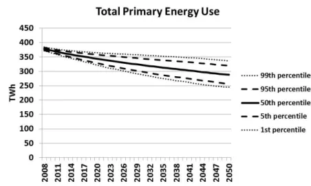
Figure 1: Global variations of Total Primary Energy Use
(presented below) showed that the non-linearities found in the model were such that no further analysis was necessary.
4. Results
4.1. Global uncertainty
The median output value for residential sector energy demand over all Monte Carlo simulations falls steadily from 378 TWh in 2008 to 344 TWh in 2020 (-9%) and 288 TWh in 2050 (-24%).
Uncertainty increases over time: the standard deviation of the output dis-tribution is increasing, while the mean is decreasing. This may be due to a propagation of the uncertainty attached to those inputs that parameterize the dynamics of the model, e.g., learning and information rates. Overall, uncer-tainty in primary energy use to 2050 is 25% at the 95% confidence level.
4.2. Important inputs
In Figure 2, inputs are ranked on the horizontal axis according to their influence on the output in 2020, measured as their µ∗ value on the vertical axis.
We see that uncertainty is concentrated among a handful of inputs. A similar observation can be made for the long-term output (not reported here). Such a concentration is quite common in sensitivity analysis (Saltelli et al., 2008). In the following discussion, we focus on the 10 most important inputs for each of the two outputs examined (Tables 1 and 2). This leads us to identify 13
long. Running Res-IRF on a standard computer with CPU of 2.6 GHz and 4 Gb of RAM takes approximately one minute
Figure 2: Input influence on Total Primary Energy Use to 2020
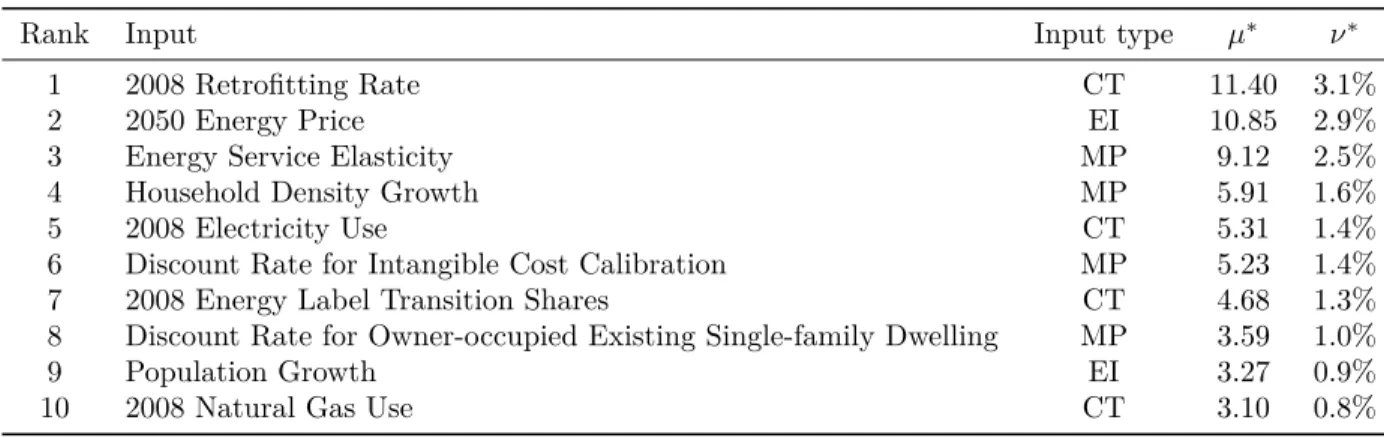
Table 1: Inputs most influential on Total Primary Energy Use to 2020 (EI: exogenous input; CT: calibration target; MP: model parameter)
Rank Input Input type µ∗ ν∗
1 2008 Retrofitting Rate CT 11.40 3.1%
2 2050 Energy Price EI 10.85 2.9%
3 Energy Service Elasticity MP 9.12 2.5%
4 Household Density Growth MP 5.91 1.6%
5 2008 Electricity Use CT 5.31 1.4%
6 Discount Rate for Intangible Cost Calibration MP 5.23 1.4%
7 2008 Energy Label Transition Shares CT 4.68 1.3%
8 Discount Rate for Owner-occupied Existing Single-family Dwelling MP 3.59 1.0%
9 Population Growth EI 3.27 0.9%
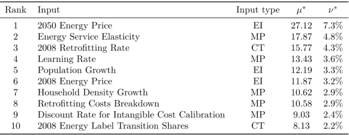
Table 2: Inputs most influential on Total Primary Energy Use to 2050 (EI: exogenous input; CT: calibration target; MP: model parameter)
Rank Input Input type µ∗ ν∗
1 2050 Energy Price EI 27.12 7.3%
2 Energy Service Elasticity MP 17.87 4.8%
3 2008 Retrofitting Rate CT 15.77 4.3%
4 Learning Rate MP 13.43 3.6%
5 Population Growth EI 12.19 3.3%
6 2008 Energy Price EI 11.87 3.2%
7 Household Density Growth MP 10.62 2.9%
8 Retrofitting Costs Breakdown MP 10.58 2.9%
9 Discount Rate for Intangible Cost Calibration MP 9.03 2.4%
10 2008 Energy Label Transition Shares CT 8.13 2.2%
important inputs. To get a more tangible value of importance, we also compute
ν∗, the ratio between µ∗and the output value in the reference scenario. A value
of 2% for ν∗
i means that a change of △ (which is close to 0.5) of input i (assumed
to be uniformly distributed in [0,1]) leads, on average, to a 2%/△ increase in the output value, as compared to its value in the reference scenario.
Three inputs consistently stand out as being most influential: the 2050 en-ergy price, the 2008 retrofitting rate and the enen-ergy service elasticity. The 2050 energy price is an exogenous input, which is mostly influential in the long-term. The 2008 retrofitting rate is the target against which the retrofitting function is calibrated. It proves to be most influential in the short-term. The energy service elasticity is a model parameter.
After these three most influential inputs, the learning rate proves to be influ-ential in the long-term, which is consistent with it parameterizing an accumu-lation process. The 2008 energy price has a significant impact in the long-term, but hardly any impact in the short-term. This perhaps counter-intuitive out-come is in fact due to the calibration of the retrofitting function, as will be shown further on in the analysis. The discount rate used to calibrate intangible costs is influential in both the short- and long-term. The discount rate parameterizing the investment behavior of owner-occupiers of existing singe-family dwellings (the biggest category of decision-makers) is influential in the short-term.
The breakdown of retrofitting costs (see AppendixC) is among the top ten most influential inputs in the long-term. Part of its influence is absorbed by the variations of intangible costs in the short-term. In the long-term, as the latter vanish, the variations of investment costs become more visible.
The 2008 Energy label transition share input is also influential. Together with the influence of the 2008 retrofitting rate, this emphasizes the importance of calibration targets. The population growth and the household density growth, which are directly linked to the floor area of new dwellings to be built each year, are also significant. Finally, two building stock calibration targets are
important: the 2008 demand for electricity and natural gas.
4.3. Robustness of the ranking
Two questions arise: is computing 80 elementary effects per input enough to get reliable estimates of µ∗? Would the ranking change if we had more
trajectories? To answer these questions, we compute the position factor index defined by Ruano et al. (2012):
P Fri→rj = k X l=1 |Pl,i− Pl,j| 0.5 × (Pl,i+ Pl,j)
where Pl,iis the position of input l when r = ri.
The P Fri→rj index measures the difference between rankings obtained with
samples of size ri and rj. The paramaters found to be most sensitive are given
higher weight in the index. A low value of P F (e.g. less than 2) means that the ranking is robust to an increase in the sample size. However, the P F value may increase as sample sizes increase. Thus in the present analysis, we consider a ranking to be stable when P F indices of a parameter tested over a range of sample sizes are all found to have low values.
As shown in Table 3, the position factor indices are found to be consistently low. They are even below 1 when the number of trajectories is shifted from 70 to 80. Whatever the shift examined, the indices tend to be higher when applied to the long-term output as compared to the short-term one. This seems quite logical because as the time horizon gets further away, the chances are greater that an input will become influential and thus change its ranking. Overall, the sensitivity analysis suggests that the ranking obtained in the previous section is robust9.
Table 3: Position Factor Index
30 to 40 40 to 50 50 to 60 60 to 70 70 to 80
2020 Energy Use 1.82 1.31 0.46 0.51 0.87
2050 Energy Use 2.24 1.95 2.27 1.91 0.68
4.4. Linearity, monotony and stability of the model
One strength of the Morris method is to give a sense of the nonlinearity of model inputs, that is, the extent to which they interact with each other10.
9
For each input, a higher σ means a greater variability of elementary effects. In this case more elementary effects are needed to get an accurate estimate of µ. The efficiency of the Morris method could thus be improved by adjusting the number of elementary effects computed for each input to its σ value. Such a refinement goes beyond the scope of this article.
10
Unlike the Sobol method, the Morris method does not track interactions. That is, it provides an aggregate measure of the interactions between one input and all others, but does
Figure 3: Morris diagram of inputs affecting Total Primary Energy Use to 2020
Input nonlinearities can be visualized in so-called Morris diagrams, as shown in Figures 3 and 4. Each diagram displays, for each of the 13 most important inputs, the standard deviation of elementary effects σ plotted against the mean
µ∗. The dotted line σ = µ∗ partitions the space. Inputs located in the upper
left space are deemed to be nonlinear. A high value of σ relative to µ∗indicates
strong interactions of the associated input with other inputs. Inputs located in the lower right space are deemed to be linear.
Three inputs stand out as being nonlinear: the discount rate used to cali-brate intangible costs, the one used by owner-occupiers of existing singe-family dwellings, and the retrofitting costs breakdown. These inputs can be seen as different degrees of freedom in the calibration of intangible costs. It is thus coherent that they interact with other inputs. Overall, there are only a few nonlinear inputs and their degree of nonlinearity is relatively low. Therefore, the Morris method has proved to be both relevant and sufficient for a sensitivity analysis of Res-IRF.
Another strength of the Morris method is to give a sense of the monotony of input influence. This can be approximated, for each input, by the value of the µ/µ∗ ratio. A value of 1 (resp. -1) indicates that an increase in the input
value always induces an increase (resp. decrease) in the output, regardless of the values of the other inputs. Table 4 displays the monotony of the 13 most influential inputs based on their µ/µ∗ ratios in 2020 and 2050.
Table 4: Monotony of most influential inputs as related to Total Primary Energy Use
Input Monotony
2050 Energy Price negative
Energy Service Elasticity negative
2008 Retrofitting Rate negative
Learning Rate negative
Population Growth positive
2008 Electricity Use positive
2008 Natural Gas Use positive
2008 Energy Price positive
Household Density Growth negative
Discount Rate for Owner-occupied Existing single-family dwellings ambiguous
Retrofitting Costs Breakdown ambiguous
Discount Rate for Intangible Cost Calibration ambiguous
2008 Energy Label Transition Shares negative
Some relations are unambiguous and intuitive. The higher any of the 2050 energy price, the 2008 retrofitting rate, the learning rate or the 2008 energy label
transition shares, the larger the number of retrofits and the lower the energy use. On the other hand, the higher any of the 2008 electricity and natural gas demands or the population growth, the higher the energy use. In contrast, the effects of inputs related to retrofitting costs and intangible costs are ambiguous. A perhaps counterintuitive result is the positive relation between the 2008 energy price and energy use. It can however be explained by the calibration of the retrofitting function to year 2008. All else being equal, a higher energy price at the calibration step implies a higher net present value associated with a retrofit, hence a lower number of retrofits per unit of profitability in the retrofitting function. In subsequent model dynamics, fewer retrofits lead to a higher energy use.
The shares of energy label transitions in 2008 also exhibits a counterintu-itive monotony. A higher value of this input reflects a world with more energy efficient retrofits in the initial year than in the reference scenario. Replication of such a world in the calibration process leads to lower intangible costs. If ini-tial intangible costs are lower, their potenini-tial for decrease through information spillovers is also lower. In the short- and long-term, this ultimately leads to less energy savings.
One last strength of the Morris method is that the simulation sequence is not impaired by computation crashes. Computation crashes are hard to avoid in sensitivity analysis, as the calibration step involves the resolution of very non-linear systems. The analysis reported here had a failure rate of 2.2%, that is, 124 crashes happened out of 5,760 simulations. This led us to exclude 138 elementary effect calculations11. Figure 5 displays the distribution of crashes
over the set of inputs. It shows that the excluded elementary effects were not confined to a handful of inputs. No input had more than nine elementary effects excluded out of 80 calculated and most had less than five excluded. Therefore, the low number of crashes experienced in the analysis did not introduce any statistical bias in the results.
5. Discussion
5.1. Fitness for purpose of the model
Sensitivity analysis allows modelers to assess the “fitness for purpose” of a model. This can be seen as a heuristic judgement of its quality (Saltelli et al., 2008). The purpose of Res-IRF is to improve behavioral detail in residential sector energy-economy modeling. Several of the model’s features are designed to serve this purpose: an endogeneization of the extensive margin of energy efficiency investment, calibrated against the initial retrofitting rate; the uti-lization of energy carrier, parameterized with an energy service elasticity; the introduction of some barriers to energy efficiency investments.
11
Apart from the first and last simulations of a trajectory, each simulation is used for two elementary effects calculations. One isolated crash then implies the exclusion of two elemen-tary effect calculations. However, if n simulations crash sequentially, only n + 2 calculations are excluded. In the analysis reported here, most crashes occurred sequentially.
Figure 5: Distribution of excluded elementary effects among inputs The fact that the initial retrofitting rate and the energy service elasticity are both found to be among the most influential inputs suggests that disaggre-gating the different drivers of energy use is a relevant modeling choice. The importance found for these inputs is consistent with the energy price being the most influential input. As it impacts all three margins of energy use, it prop-agates the variability attached to each. Though theoretically uncontroversial, disaggregating different energy drivers is empirically challenging. In particular, data is needed to make a better estimation of the initial retrofitting rate and the energy service elasticity.
In contrast, the barriers to energy efficiency introduced in the model have been found to have little influence. This is notable for discount rates, which is at odds with the importance they have been reported to have in most other models12. As using discount rates to mimic barriers to energy efficiency raises
theoretical and empirical concerns first reported by (Jaffe and Stavins, 1994), the finding of low-influence is perhaps not so problematic. Therefore, if we are to improve behavioral detail in the modeling of residential sector energy demand, a basic disaggregation of the different drivers of energy use should be prioritized over focus on a more elaborate incorporation of barriers to energy efficiency.
5.2. Unaddressed uncertainty
The Morris method has allowed us to fully explore the input space. Though such an analysis may give an impression of completeness, it does not clear all sources of uncertainty. The delimitation of the variation in input space by the
12
Note that the discount rate variations examined in this paper are centered around higher values than those typically examined in integrated assessment models, which usually vary in the [0%,8%] range. This explains partly the lower influence for discount rates found in our analysis.
modeler involves some arbitrary assumptions. So too does the choice of outputs examined. Some outputs that were not examined in this paper may be affected by inputs that were in this work not found to have much influence. Lastly, beyond numbers, the uncertainty embodied in the functional forms and scope of the model can simply not be accounted for in a sensitivity analysis (Oreskes, 1998; Rotmans and van Asselt, 2001).
6. Conclusion
In this paper, we have discussed a sensitivity analysis of Res-IRF, a simu-lation model of energy use for space heating in French dwellings. We used the Morris method of sensitivity analysis, which to date has not been widely used by the energy-economy modeling community. 5,760 simulations were run to assess the influence of all 71 model inputs. We found global uncertainty to be within the acceptable range: the main output of interest, Total Primary Energy Use to 2050 varies by 25% at the 95% confidence level. We also found the model to be quite stable: less than 3% of the simulations crashed. Most inputs have a linear and monotonic influence on the outputs of interest and the polarity of influence is consistent with intuition. Moreover, nearly all exogenous inputs make it among the top most influential inputs, with energy prices ranking first. This means that even though the internal structure of the model accounts for some variability, the model is mainly determined by its exogenous inputs. Thus we conclude that the reliability of the model is good. Disaggregating the three drivers of energy use also proved to be a relevant modeling choice. Although sensitivity analysis seems like a very obvious thing to do for this kind of en-ergy system modelling, it is rarely done in peer models, probably because it is technically challenging.
These conclusions, retrospectively, give more substance to the results in previous work (Giraudet et al., 2011a). The takeaway of that work can be summarized as follows: there are technical and behavioral rigidities that affect energy-related decisions which make ambitious carbon dioxide emissions reduc-tions targets in the residential sector difficult to meet in the near future. Other models have reached the same conclusions (see AppendixA for a review). They thus provide an external corroboration of the model which complements the internal corroboration provided by the sensitivity analysis carried out in this work.
Our evaluation suggests some directions for model development. First, many inputs proved to be unimportant in the sensitivity analysis. Res-IRF could be simplified accordingly. For instance, the growth in floor area per capita could be modelled to follow an exogenous trend rather than respond to GDP growth. Second, data is needed to make a better estimation of the empirical parameters identified as being most important. This applies to the retrofitting rate in particular. Third, the analysis revealed that Res-IRF was not very sensitive to variations in representations of the barriers to energy efficiency. However, this point is controversial, both from a theoretical and empirical point of view. Therefore, more research is needed to clarify which barriers should be described
in detail in models of energy demand, before concluding the sensitivity of these models to such barriers.
References
ADEME (2009). Evaluation prospective du marché du chauffage domestique au bois et autres biomasse en 2020. Technical report.
Allcott, H. and Greenstone, M. (2012). Is there an energy efficiency gap?
Jour-nal of Economic Perspectives, 26(1):3–28.
Bellmann, R. E. (1957). Dynamic Programming-Code. Princeton University Press.
Bibas, R., Mathy, S., and Fink, M. (2012). Building a low carbon scenario for france. how a participatory approach can enhance social and economic acceptability. Technical report, ENCI-LowCarb Project.
Braddock, R. D. and Schreider, S. Y. (2006). Application of the morris algo-rithm for sensitivity analysis of the REALM model for the goulburn irrigation system. Environmental Modeling & Assessment, 11(4):297–313.
Campolongo, F. and Braddock, R. (1999). Sensitivity analysis of the IMAGE greenhouse model. Environmental modelling & software, 14(4):275–282. Campolongo, F., Cariboni, J., and Saltelli, A. (2007). An effective screening
design for sensitivity analysis of large models. Environmental Modelling &
Software, 22(10):1509–1518.
Campolongo, F., Kleijnen, J., and Andres, T. (2000). Screening methods. In
Sensitivity Analysis, pages 65–80. John Wiley & Sons, Ltd, New York.
Campolongo, F., Saltelli, A., and Cariboni, J. (2011). From screening to quan-titative sensitivity analysis. a unified approach. Computer Physics
Commu-nications, 182:978–988.
Cayre, E., Allibe, B., Laurent, M.-H., and Osso, D. (2011). There are people in the houses! how the results of purely technical analysis of residential energy consumption are misleading for energy policies. Proceedings of the ECEEE
2011 Summer Study, pages 1675–1683.
Charlier, D. and Risch, A. (2012). Evaluation of the impact of environmental public policy measures on energy consumption and greenhouse gas emissions in the french residential sector. Energy Policy, 46:170–184.
Confalonieri, R., Bellocchi, G., Bregaglio, S., Donatelli, M., and Acutis, M. (2010). Comparison of sensitivity analysis techniques: A case study with the rice model WARM. Ecological Modelling, 221(16):1897–1906.
Cooling, M., Hunter, P., and Crampin, E. J. (2007). Modeling hypertrophic IP3 transients in the cardiac myocyte. Biophysical Journal, 93(10):3421–3433. Energy Modeling Forum, S. U. (2011). Energy efficiency and climate change
mitigation. Technical Report Report 25, Energy Modeling Forum, Stanford University.
Garcia Sanchez, D., Lacarrière, B., Musy, M., and Bourges, B. (2014). Ap-plication of sensitivity analysis in building energy simulations: Combining first- and second-order elementary effects methods. Energy and Buildings, 68:741–750.
Gillingham, K. T., Newell, R. G., and Palmer, K. (2009). Energy efficiency economics and policy. Annual Review of Resource Economics, 1(1):597–620. Giraudet, L.-G., Guivarch, C., and Quirion, P. (2011a). Comparing and
com-bining energy saving policies: Will proposed residential sector policies meet french official targets? The Energy Journal, 32(01).
Giraudet, L.-G., Guivarch, C., and Quirion, P. (2012). Exploring the potential for energy conservation in french households through hybrid modeling. Energy
Economics, 34(2):426–445.
Giraudet, L.-G., Guivarch, C., Quirion, P., and Penot-Antoniou, L. (2011b). Evaluation des mesures du grenelle de l’Environnement sur le parc de loge-ments. Technical Report 58, Commissariat général au développement durable. Giraudet, L.-G. and Quirion, P. (2008). Efficiency and distributional impacts of tradable white certificates compared to taxes, subsidies and regulations.
Revue d’économie politique, Vol. 118(6):885–914.
Hourcade, J.-C., Jaccard, M., Bataille, C., and Ghersi, F. (2006). Hybrid mod-eling: New answers to old challenges introduction to the special issue of the energy journal. The Energy Journal, SI2006(01).
INSEE (2008). Comptes du logement. Technical report, INSEE.
Iooss, B. (2011). Revue sur l’analyse de sensibilité globale de modèles numériques. Journal de la Société Fran\ccaise de Statistique, 152(1):3–25. Jaccard, M. and Dennis, M. (2006). Estimating home energy decision
parame-ters for a hybrid energy—economy policy model. Environmental Modeling &
Assessment, 11(2):91–100.
Jaffe, A. B. and Stavins, R. N. (1994). The energy-efficiency gap what does it mean? Energy Policy, 22(10):804–810.
Kavgic, M., Mavrogianni, A., Mumovic, D., Summerfield, A., Stevanovic, Z., and Djurovic-Petrovic, M. (2010). A review of bottom-up building stock models for energy consumption in the residential sector. Building and
Levine, M., Ürge Vorsatz, D., Blok, K., Geng, L., Harvey, D., Lang, S., Lev-ermore, G., Mongameli Mehlwana, A., Mirasgedis, S., Novikova, A., Rilling, J., and Yoshino, H. (2007). 2007: Residential and commercial buildings. In Metz, B., Davidson, O., Bosch, P., Dave, R., and Meyer, L., editors, Climate
Change 2007: Mitigation. Contribution of Working Group III to the Fourth Assessment Report of the Intergovernmental Panel on Climate Change.
Cam-bridge University Press, CamCam-bridge, United Kingdom and New York, NY, USA.
Marchal, J. (2008). Modélisation des performances thermiques du parc de loge-ments. Technical report, ANAH.
Matthews, C. J., Newton, D. B., Braddock, R. D., and Yu, B. (2006). Analysing the sensitivity behaviour of two hydrology models. Environmental Modeling
& Assessment, 12(1):27–41.
Mau, P., Eyzaguirre, J., Jaccard, M., Collins-Dodd, C., and Tiedemann, K. (2008). The ‘neighbor effect’: Simulating dynamics in consumer preferences for new vehicle technologies. Ecological Economics, 68(1–2):504–516.
McKinsey (2009). Unlocking energy effi - ciency in the U.S. economy. Technical report.
Morris, M. D. (1991). Factorial sampling plans for preliminary computational experiments. Technometrics, 33(2):161–174.
Mundaca, L., Neij, L., Worrell, E., and McNeil, M. (2010). Evaluating energy ef-ficiency policies with energy-economy models. Annual Review of Environment
and Resources, 35(1):305–344.
OMB (2013). Informing regulatory decisions: report to congress on the costs and benefits of federal regulations and unfunded mandates on state, local, and tribal entities. Technical Report Appendix D, OMB Circular A-4. OPEN (2009). Rapport final. Technical report, Observatoire permanent pour
l’amélioration énergétique du logement.
Oreskes, N. (1998). Evaluation (not validation) of quantitative models.
Envi-ronmental Health Perspectives, 106 (6):1453–1460.
Potting, J., Heuberger, P., Beusen, A., van Vuuren, D., and de Vries, B. (2002). Sensitivity analysis. In Uncertainty assessment of the IMAGE/TIMER B1
CO2 emissions scenario, using the NUSAP method. Dutch National Research
Programme on Global Air Pollution and Climate Change.
Richter, G. M., Acutis, M., Trevisiol, P., Latiri, K., and Confalonieri, R. (2010). Sensitivity analysis for a complex crop model applied to durum wheat in the mediterranean. European Journal of Agronomy, 32(2):127–136.
Rotmans, J. and van Asselt, M. B. A. (2001). Uncertainty management in inte-grated assessment modeling: towards a pluralistic approach. Environmental
monitoring and assessment, 69(2):101–130.
Ruano, M. V., Ribes, J., Seco, A., and Ferrer, J. (2012). An improved sampling strategy based on trajectory design for application of the morris method to systems with many input factors. Environmental Modelling & Software. Saltelli, A. and Annoni, P. (2010). How to avoid a perfunctory sensitivity
analysis. Environmental Modeling and Software, 25:1508–1517.
Saltelli, A., Ratto, M., Andres, T., Campolongo, F., Cariboni, J., Gatelli, D., Saisana, M., and Tarantola, S. (2008). Global Sensitivity Analysis: The
Primer. Wiley.
Sobol, I. (1993). Sensitivity analysis for non linear mathematical models.
Math-ematical modelling and computational experiment, 1:407–414.
Tang, Y., Reed, P., Wagener, T., and Werkhoven, K. v. (2007). Comparing sen-sitivity analysis methods to advanced lumped watershed model identification and evaluation. Hydrology and Earth System Sciences, 11:793–817.
Wilkerson, J. T., Cullenward, D., Davidian, D., and Weyant, J. P. (2013). End use technology choice in the national energy modeling system (NEMS): an analysis of the residential and commercial building sectors. Energy Economics, 40:773–784.
AppendixA. Preliminary Assessment of Res-IRF
Res-IRF’s defining paper contained a preliminary evaluation of the model (Giraudet et al., 2012). The numerical values generated in the reference sce-nario proved consistent with those commonly found in the literature for such variables as the growth rate of the building stock, the rebound effect and the price-elasticity of energy demand. Local sensitivity analysis was conducted on a few parameters suspected to be influential: energy prices, information spillovers, the learning-by-doing rate, discount rates and the heterogeneity parameter. This analysis revealed that the information spillovers and the heterogeneity parame-ters had a significant impact on the retrofitting rate; the impact of the learning-by-doing rate and the discount rate was low and the impact of energy prices even lower. However, the impact of the energy price on final energy use was high, whereas the impact of all other inputs was low. This illustrates the fact that the energy price has an impact on both energy efficiency investment and capital utilization. In contrast, the impact of other inputs on energy efficient retrofits is partly taken back by the rebound effect.
Res-IRF has been used with the support of the French Sustainable Develop-ment General Commission to simulate the effectiveness of policies targeting the
French residential building sector (Giraudet et al., 2011b). A carbon tax, sub-sidies (income tax credits and zero interest rate loans for energy retrofits) and regulations (stringent building codes for new buildings and retrofitting obliga-tions in existing buildings) were assessed against the national targets of reducing energy use in existing buildings by 38% in 2020 compared to 2008, and dividing CO2 emissions by four in 2050 compared to 1990. The analysis revealed that
taxes were the most effective instrument to lower final energy use, although it was the least effective at increasing energy efficiency investment. This result is consistent with insights from microeconomic optimization models (e.g., Gi-raudet and Quirion (2008)). It rests on the same drivers as those exhibited in the local sensitivity analysis of the model: as all policy instruments improve energy efficiency, thereby generating a rebound effect, carbon taxes impact at the same time capital utilization. The main insight from this policy assessment was that national targets were unlikely to be met, unless policies were set far out of the range discussed in the policy arena13.
Comparing Res-IRF to peer models sheds an external light on its reliabil-ity. Charlier and Risch (2012) developed a bottom-up model of energy demand in French residential buildings which lends itself to such a comparison. Their model shares commonalities with Res-IRF: the retrofitting rate is endogenous and landlord-tenant split incentives are modeled through heterogeneous pay-back times among decision-makers. Yet the two models have different strengths. Charlier and Risch’s model (hereafter the CR model) incorporates greater tech-nological detail than Res-IRF: it is fed by outputs of an engineering model of building energy use, which takes into account explicit technologies for heating and hot water, appliances and lighting uses. It also incorporates rich statistical data on household characteristics, such as income and debt ratio (in addition to the tenancy characteristics mentioned above). On the other hand, in the CR model, capital utilization is held constant and there are neither intangible costs nor dynamic effects such as learning-by-doing or information spillovers. The reference scenarios in both models cannot be compared easily: while both are based on the same population growth projected by INSEE, they assume quite contrasted energy price scenarios, increasing at an annual rate of 3.3% in the CR model and 0.5% in Res-IRF. Models respond to these reference scenarios by a decrease in specific primary energy use through 2050 of 48% in the CR model and 23% in Res-IRF. Charlier and Risch also conducted an assessment of various types of subsidies to meet national targets. They find a higher effectiveness of subsidies than in Res-IRF. One possible explanation for this higher sensitivity is the absence of an endogenous rebound effect in the CR model. Despite their differences, both models share the conclusion that national targets are unlikely to be met with current policies.
Res-IRF was involved in the Energy Modeling Forum’s 25th study, focusing
13
Supplementary analysis by the French Sustainable Development General Commission, taking into account some levies not included in the model, confirmed this conclusion (Giraudet et al., 2011b).
on energy efficiency (Energy Modeling Forum, 2011). The study involved a va-riety of top-down and bottom-up energy-economy models, mostly focusing on the U.S. economy, which were run with standardized assumptions. Compared to other models, sensitivity to energy efficiency policy in Res-IRF14 proved
in-termediate. The model, however, exhibited two distinct behaviors. First, the relative impact of a carbon tax on residential energy intensity was almost the largest of all models (Ibid., Figure 10). Again, this is likely driven by the en-dogenous representation of capital utilization, a feature exclusive to Res-IRF in the study. Second, unlike other models, Res-IRF exhibited some slightly over-additive interactions when a carbon tax was combined with energy efficiency standards (Ibid., Figure 15). A decomposition of this stylized fact at the time of the study revealed that it was driven by the logistic shape of the retrofitting curve. As the model and policies were parameterized, most retrofits were occur-ring in the convex region of the logistic curve; therefore, an increase in the net present value of retrofitting translated into a more-than-proportional increase in the number of retrofits. Beyond this specific result, the key finding of the study was that regardless of the top-down or bottom-up nature of the models involved, all exhibited rigidities that made the attainment of ambitious carbon dioxide emissions reductions through energy efficiency much harder than those found in pure engineering studies, as exemplified by the widely discussed Mc Kinsey study (McKinsey, 2009).
The main takeaway from this preliminary assessment is that Res-IRF results seem plausible, at least compared to past trends and to other models. Still, its main distinctive features, especially information spillovers, capital utilization and retrofitting dynamics proved influential, which motivated the subsequent analysis reported in the present paper.
AppendixB. Model updates
This section updates the description of the model, which was first published in Giraudet et al. (2012).
AppendixB.1. Data refinement
New corrections have been applied to the database of Marchal (2008) to take better account of secondary residence and vacant units, and match the proportion of landlords and tenants with data from INSEE (2008). Based on the OPEN survey (OPEN, 2009), the initial retrofitting rate has been re-estimated at 3%/year instead of 1%/year. Expert elicitation have led to a downward revision of estimates of retrofitting costs (Table 2 in Giraudet et al. (2012)); the
14
In that study, Res-IRF was linked to IMACLIM-R France. This overarching framework was simply named “IMACLIM” in the study.
cost matrix is now (in e/m2): CIN V−0= 76 136 201 271 351 442 0 63 130 204 287 382 0 0 70 146 232 331 0 0 0 79 169 271 0 0 0 0 93 199 0 0 0 0 0 110
Social housing has been introduced with a 4% discount rate, a value meant to reflect public decision-making. Other discount rates have been adjusted so as to maintain the weighted average discount rate at 20%. The new values are: 8% in owner-occupied single-family dwelling, 15% in owner-occupied multi-family dwellings, 45% in rented single-family dwellings, and 55% in rented multi-family dwellings.
AppendixB.2. Introduction of fuel wood and social housing
Fuel wood has been introduced as a new heating fuel and social housing has been introduced as a new dwelling type. Social housing was directly parame-terized from Marchal (2008). In Marchal’s database, fuel wood is mixed with all fuels other than natural gas, electricity and fuel oil in a single category. To match this with data from ADEME (2009), it was assumed that 44% of single-family dwellings and 1% of multi-single-family dwellings in this category were heated with fuel wood.
Fuel wood dwellings are assumed to account for 9% of new dwellings, and social housing 20%. The other categories are adjusted to keep initial proportions (Table 11 in Giraudet et al. (2012)).
Adding a fuel led to an additional row in the matrix of construction costs (Table 8 in Giraudet et al. (2012)). The new row reads as follows: 1200 e/m2
for constructions meeting the 2005 building code, 1300 e/m2 for constructions
meeting the 2012 building code and 1600 e/m2 for constructions meeting the
2020 building code.
A column and a row were added to the matrix of fuel switch costs (Table 7 in Giraudet et al. (2012)): 0 70 100 120 50 0 80 100 55 50 0 100 55 50 80 0
From ADEME (2009), the initial price of fuel wood in 2007 was assumed to be 0.04 e/kWh. The initial floor area in social housing was assumed to be 60 m2 in existing dwellings and 65 m2 in new dwellings. A saturation is placed at
AppendixB.3. Energy Service Function
In the previous version of the model (equation (14) Giraudet et al. (2012)), a logistic energy service function was estimated using data from (Cayre et al., 2011). Here, the same data was fitted with an iso-elastic relationship, which is more convenient for subsequent sensitivity analysis: It is easier to vary a constant elasticity than the multiple parameters of a logistic function. The function Fk(P ) = K(ρkP )e was estimated, with P the price of energy and ρk
the inverse efficiency parameter for a dwelling of type k. With ten points (yi, di) where yiis the utilization rate and dithe theoretical expenditure, a log-log linear
regression yielded K = 2.72 and e = −0.505.
AppendixC. Indirect inputs used in sensitivity analysis
Some inputs of the model cannot be directly submitted to sensitivity analysis for a variety of reasons. Indirect inputs are built to circumvent this problem.
AppendixC.1. Exogenous inputs
Population, GDP and energy prices follow exogenous trajectories. One com-mon way to assess the influence of input trajectories is to assess sensitivity to a constant annual growth rate. Yet such a factor potentially leads to very high values at the end of the time horizon. We adopt a different approach in our sensitivity analysis.
Each energy price trajectory is parameterized by two random inputs: the short-term price (in 2008) and the long-term price (in 2050). The energy price evolves linearly between these two values over the 2008-2050 period. The energy price value disclosed in table D.5 is for natural gas; the growth pattern is parallel for other fuels.
For the population trajectory, we build a random growth input ξ corre-sponding to a percentage increase growing over time. The reference values are multiplied by [1 + (1 + (Y ear − 2008)/10)ξ]. With proceed similarly with the GDP trajectory.
AppendixC.2. Initial capital stock
Initial capital stock is, together with the learning rate, the input that pa-rameterizes the learning-by-doing process. It is labeled Kf(0) in equation (7)
in Giraudet et al. (2012). It is given in the model as a hypermatrix and varied in the sensitivity analysis by a scalar k as follows: Kf(0)(1 + k).
AppendixC.3. Calibration Targets: Shares
All 2008 shares to be replicated by the model (Energy label transitions in existing dwellings, energy labels in new constructions, fuel shares in new con-structions, building type shares in new constructions) are given by matrices, the rows of which sum to 1. Sensitivity of the model to such inputs cannot be assessed by simply multiplying the associated matrix by a scalar. Matrix elements must be changed specifically. To do so, we build indirect inputs.
The matrix of 2008 energy label transitions against which intangible costs are calibrated is:
M Sini= 25% 27% 27% 21% ε% ε% 40% 26% 31% 2% ε% 66% 28% 6% ε% 95% 5% ε% 91% 9% 100%
For instance, 26% of the dwellings in energy label F reach label C after retrofit. We build an indirect input α that represents the relative efficiency of 2008 energy label transitions: the higher α, the larger the proportion of transitions toward high energy labels. Input α is symmetric around 0, with negative values reflecting a less energy efficient situation than in the reference situation.
If α is positive, we make the following transformation:
a′ i,i= ai,i(1 − α) and: a′i,j= ai,j+ ai,j 1 − ai,i αai,i for i < j.
For α = 0.5, we thus have:
M Sini= 12% 31% 31% 24% ε% ε% 20% 35% 42% 3% ε% 33% 55% 12% ε% 47% 52% ε% 46% 55% 100%
If α is negative, we make the following transformation:
a′i,i= ai,i+ (1 − ai,i)|α|
and:
a′i,j= (1 − |α|)ai,j
M Sini= 62% 13% 13% 10% ε% ε% 70% 13% 16% 1% ε% 83% 14% 3% ε% 98% 2% ε% 95% 5% 100%
We build a similar input to assess sensitivity of the model to the matrix of initial market shares of new constructions.
For fuel shares and building type shares, we adopt a slightly different ap-proach. We assess sensitivity to one element of the matrix and adjust other elements so that the matrix sums to 1. For instance, for fuel shares, we vary the electricity share through indirect input optelec:
M Selec= (1 + optelec)M Selec
We then adjust the shares of other fuels and multiply them by the same scalar λ:
M Si′6=elec= λM Si6=elec
Solving equation P M Si= 1, we find: λ = 1 − M Selec
1 − M Selec optelec AppendixC.4. Retrofitting Costs
Retrofitting costs, that is, energy label transition costs are given in the model as a matrix. We assess the sensitivity of the model to the cost magnitude through a scalar multiplying the matrix. We also assess the sensitivity of the model to the cost breakdown by multiplying the matrix term by term to the following matrix: 1 1 +γ 5 1 + γ 4 1 + γ 3 1 + γ 2 1 + γ 1 + γ 5 1 + γ 4 1 + γ 3 1 + γ 2 1 + γ 1 +γ 4 1 + γ 3 1 + γ 2 1 + γ 1 +γ 3 1 + γ 2 1 + γ 1 + γ 2 1 + γ 1 + γ
Indirect input γ, if positive, gives relatively more weight to very energy efficient transitions; it gives them relatively less weight if negative.
AppendixC.5. 2008 Existing Building Stock Factors
The number of existing dwellings in 2008, given as a hypermatrix in the model, is broken down by energy label (labels G to A), heating fuel (electricity, natural gas, fuel oil and fuel wood) and building type (owner-occupied single-and multi-family dwellings, rented single- single-and multi-family dwellings single-and social housing).
The influence of each heating fuel is assessed by a scalar multiplying the number of dwellings in the same fuel category. The influence of building types is assessed in a similar way.
The influence of energy labels is assessed in a more aggregate way, using indirect input κ. The higher κ, the larger the proportion of high energy classes in the housing stock compared to the reference situation. Input κ keeps the number of dwellings labelled C unchanged and changes other labels as follows: label A numbers are multiplied by 1 + κ/2, label B numbers by 1 + κ, label D numbers by 1 − κ, label E numbers by 1 − κ/2, label F numbers by 1 − κ/3 and label G numbers by 1 − κ/4.
AppendixC.6. Energy Service Elasticity
The energy service is given by the following function: y = Kde, with y
the capital utilization rate, d the conventional energy expenditure and e the elasticity of utilization to conventional expenditure. Each time we vary e in the sensitivity analysis, we need to re-estimate K to best fit the data.
We introduce function f (k) = 10 X i=1 [ln(yi) − (k + eln(di))]2
which is the sum of squared distances between points from the regression and real data (k = ln(K)). As e is fixed, we need to find k0which minimizes f.
We have f′(k) = −2 10 X i=1 [ln(yi) − (k + eln(di))] and f′′(K) = 2 × 10 > 0
Therefore the function is convex and has a minimum in
k0= 1 10 10 X i=1 [ln(yi) − eln(di)]