Algorithmic advances towards a fully automated DNA genotyping system

Algorithmic Advances Towards a Fully Automated

DNA Genotyping System

by

Manway Michael Liu

Submitted to the Department of Electrical Engineering and Computer

Science

in partial fulfillment of the requirements for the degree of

Master of Engineering in Electrical Engineering and Computer Science

at the

MASSACHUSETTS INSTITUTE OF TECHNOLOGY

June 2004

@

Manway Michael Liu, MMIV. All rights reserved.

The author hereby grants to MIT permission to reproduce and

distribute publicly paper and electronic copies of this thesis document

in whole or in part.

A u th or ...

...

Departme t of Electrical Engineering and Computer Science

May 20, 2004

Certified by..

...

Dan Ehrlich

Director, BioMEMS Labofraty, Center fqr Biomedical Engineering

-Thesis Supervisor

Accepted by ...

...

Arthur C. Smith

Chairman, Department Committee on Graduate Students

MASSACHUSE-TS INST E OF TECHNOLOGY

JUL 2 0 2004

Algorithmic Advances Towards a Fully Automated DNA

Genotyping System

by

Manway Michael Liu

Submitted to the Department of Electrical Engineering and Computer Science on May 20, 2004, in partial fulfillment of the

requirements for the degree of

Master of Engineering in Electrical Engineering and Computer Science

Abstract

Short Tandem Repeats (STR) genotyping is a leading tool in forensic DNA analy-sis. In STR genotyping, alleles in a sample are identified by measuring their lengths to form a genetic profile. Forming a genetic profile is time-consuming and labor-intensive. As the technology matures, increasing demand for improved throughput and efficiency is fueling development of automated forensic DNA analysis systems. This thesis describes two algorithmic advances towards implementing such a system. In particular, the algorithms address motif-matching and pattern recognition issues that arise in processing a genetic profile. The algorithms were initially written in MATLAB and later converted into C++ for incorporation into a prototype, auto-mated system.

Thesis Supervisor: Dan Ehrlich

Acknowledgments

0.1

Acknowledgements

The projects outlined and discussed in this document were done during the Fall of 2002 through the Fall of 2003 and supported supported by generous funding from the Whitehead Institute for Biomedical Research and specifically by the BioMEMS Laboratory headed by Dr. Paul Matsudaira. Project research was supervised by Dr. Dan Ehrlich, Brian McKenna, and Sameh El-Difrawy. Additionally, research assis-tant Loucinda Carey supplied much of the validation data and performed extensive validation for the automated allele calling algorithm.

Contents

0.1 Acknowledgements . . . . 3 1 Introduction 6 2 Genetics Overview 8 3 DNA Genotyping 13 3.1 Sample Preparation . . . . 13

3.2 Polymerase Chain Reaction . . . . 13

3.3 DNA Separation Electrophoresis . . . . 14

3.4 Allele Calling . . . . 16

3.5 P rofiling . . . . 16

4 Automated DNA Typing Systems 17 4.1 Automated DNA Separation Electrophoresis . . . . 17

4.1.1 Baselining . . . . 18

4.1.2 Color Correction . . . . 19

4.1.3 Peak picking . . . . 20

4.1.4 Stutter Correction . . . . 21

4.1.5 Standard Detection . . . . 22

4.2 Automated Allele Calling . . . . 23

5 Thesis Topics 24 5.1 Automated Standard Detection . . . . 24

5.1.2 The Solution Process . . . . 25

5.1.3 Search Algorithm . . . . 33

5.1.4 Analysis and Conclusion . . . . 35

5.1.5 Future Extensions . . . . 36

5.2 Automated Allele Lookup . . . . 37

5.2.1 The Problem . . . . 37

5.2.2 The Solution Process . . . . 39

5.2.3 Search Algorithm . . . . 43

Chapter 1

Introduction

DNA Forensic Analysis is the science of identifying DNA evidence obtained from a

crime scene and matching it to an individual or group of individuals. From as little evidence as a spot of blood, drop of saliva, or strand of hair, forensic investigators can identify the people involved at the scene of a crime. The impact of the science on society is significant and obvious: One only has to recall the Lewinsky scandal involv-ing former President Clinton as an example. Although questions continue regardinvolv-ing the scandal's propriety, the fact remains that the same technology used to implicate the former President is also routinely employed in many ongoing criminal cases.

Nonetheless, despite its influence, DNA forensic technology remains open to im-provement. One of the challenges facing it today is the transition towards full au-tomation. As yet, many steps in the process of identifying DNA evidence require manual analysis by trained technicians. While such systems suffice for now, they are less than desirable as the technology matures: Briefly, the significant monetary cost of training and staffing may impair adoption of the technology on a local level. Throughput also suffers as manual systems are less amenable to parallel experiments than fully automated ones.

This document describes two algorithmic advances to reduce manual analysis in the process of identifying DNA evidence. It is structured as follows: First, it provides a description of genetics, the science on which DNA forensic analysis is fundamentally based. It then moves onto an overview of the DNA typing process with particular

emphasis on automated systems. Only afterwards does it introduce and describe the algorithmic advances. For each advance, the document explains its contributions to the overall goal, details the experimental and developmental process that led to it, presents final results, and compares its performance against the original methodology.

Chapter 2

Genetics Overview

The science of genetics provides the factual basis behind DNA forensics. Genetics is the formal study of heredity. The basic, functional unit of heredity is the gene. A gene, in turn, is a protein-coding section of a long, double-stranded molecule known

as deoxyribonucleic acid, or DNA.

DNA is the hereditary material handed down from one generation to the next. A

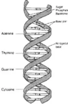
length of DNA is a sequence composed from four nucleic acids: Adenine, Thymine, Guanine, and Cytosine.

Nucleic acids on one strand of DNA complement the nucleic acids on the opposite strand with Adenine always pairing with Thymine and Guanine always pairing with Cytosine. The A-T, G-C pairings are frequently referred to as base pairs in literature. The affinity of the nucleic acids for one another, coupled with hydrogen bonding

ci.

Figure 2-1: A DNA molecule. Note the double helix structure and the base pairs

between the two strands, gives rise to the characteristic double-helix structure of

DNA. See Figure 2-1.

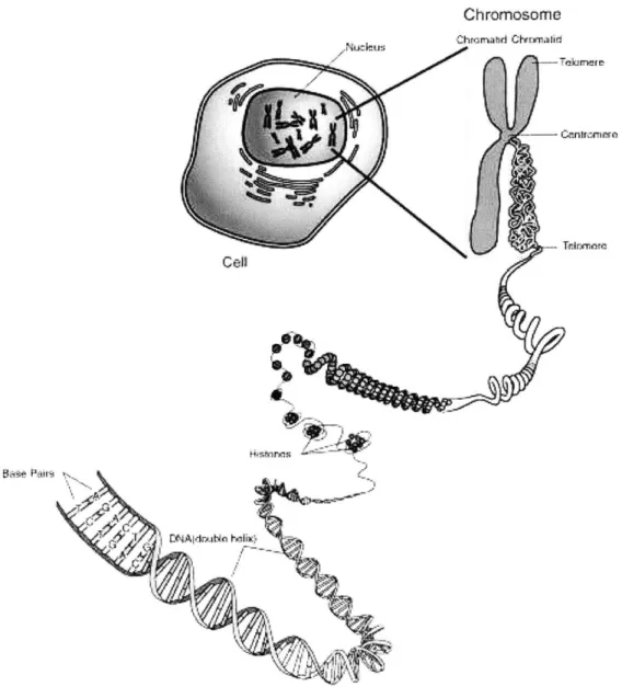
DNA is organized into chromosomes within a cell (Figure 2-2). The number of

chromosomes varies with the species. People have 46 chromosomes organized into 23 homologous pairs. Collectively, the set of chromosomes for a person constitute his genome. (Figure 2-3). An person's genome is unique; With the exception of identical twins, the genomes from two different people will differ.

Only a fraction of genomic DNA consists of genes. The majority of DNA in a genome are non-coding. DNA forensic analysis is primarily interested in genetic markers located in non-coding regions of the genome.

The term, locus, (plural loci), refers to the chromosomal location of a gene or genetic marker. With few exceptions, genetic markers are named after their loci. Variations in a genetic locus, (such as between homologous chromosomes, or between two different people), are known as alleles for that locus. Genotyping a sample implies identifying its alleles at a particular genetic locus. Forming a genetic profile for a sample requires genotyping at multiple loci.

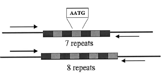
The most prevalent method of DNA forensic analysis involves identifying alleles for Short Tandem Repeats, or STRs. As the name suggests, STRs are short, 3-6 base repeating units of DNA. The base unit for a STR marker is highly conserved within a population; however, the number of times it repeats may vary, with each variation being an allele. Because alleles only differ in the number of repeats, they are distinguishable from one other based on length. (Figure 2-4).

An allele's frequency reflects its distribution in the general population. When frequencies for alleles from different genetic markers are mutually independent, the joint frequency between them is simply the product of their individual frequencies.

A genetic profile's frequency is simply the joint frequency of the identified alleles.

Hence, by testing enough genetic markers whose allelic frequencies are independent, the profile's frequency, (and by extension, the random match probability) can be made arbitrarily low.

Chromosome .Kudus hrad Crwnafid

CenT6:rena

Cell

Figure 2-2: The relationship between DNA, chromosomes, and an organism. A double-stranded DNA is bundled into small "knots" known as histones. Histones, in turn, are wounded into a tertiary coil structure. These coils are further wounded and bundled to form a chromosome. With the exception of sex chromosomes, all chro-mosomes are paired with an identical twin in a cell. People have 46 chrochro-mosomes, or

1 1 11

1I 20 21 22

Figure 2-3: The 23 pairs of chromosomes in a human that constitute its genome. This cytogenic map only shows one representative chromosome of each pair (excepting the sex chromosomes, both of which are shown). Source: National Human Genome

Research Institute.

mATG

7

repeats

8 repeats

Figure 2-4: An example STR markers with base repeat unit AATG. Notice that the alleles are polymorphic in length. While the number of repeats may differ from one

allele to the next, the repeat unit itself does not change. Generally, STR markers are chosen so that the flanking regions,

(represented

by the arrows), are conserved across alleles. Source: Short Tandem Repeat DNA Internet Database, Biotechnology

Division, NIST.

13 CODIS Core STR Loci with Chromosomal Positions

05 818 O THV FGA M 073920 I I LCSF1PO_;1 1 2 3 4 5 6 7 8 9 10 11 12 AMEL 013 D1839 D1S51 D2S11 AMEL 13 14 15 16 17 18 19 20 21 22 X Y

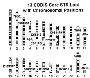
Figure 2-5: The 13 core CODIS STR loci and their chromosomal positions. CODIS is the Combined DNA Index System database maintained by the FBI and used for tracing serial crime and unsolved cases to known offenders. Source: Short Tandem

Repeat DNA Internet Database, Biotechnology Division, NIST.

into the CODIS (Combined DNA Index System) database, which is used by the FBI and other agencies in criminal investigations. (Figure 2-5). When all 13 loci are tested, the average random match probability drops below one in a trillion among unrelated individuals.

Chapter 3

DNA Genotyping

Forming a genetic profile of a sample is a multistage process. The following briefly describes the stages involved in STR genotyping.

3.1

Sample Preparation

A crime scene sample typically contains other substances besides DNA. Pure DNA

must be extracted out as cellular proteins in an impure sample can inhibit effective analysis. While methods for doing so vary depending on the characteristics of the sample, three main techniques for extracting DNA are Phenol Chloroform Extraction, Chelex Extraction, and FTA Paper Extraction. The choice of technique depends on the quality and property of the sample. For example, FTA Paper Extraction is primarily used for bloodstain analysis. Nonetheless, regardless of the technique, the output is a pure, quantified sample of DNA.

3.2

Polymerase Chain Reaction

A DNA sample is always too low-volume to give good resolution of the genetic

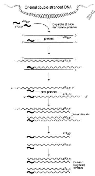
mark-ers. Polymerase Chain Reaction, or PCR, is an amplification technique that improves the yield by generating millions of copies of a sample. See Figure 3-1.

times and over multiple thermal cycles. The number of replications is exponential base 2 to the number of thermal cycles (minus the first two). Hence, after around

32 cycles, approximately one billion copies of the desired region of DNA will be

generated. The amplified amount is generally sufficient for effective analysis.

To target specific regions for amplification, short DNA sequences, known as primers, are added into the PCR process. These tailored sequences specifically bind to the

DNA sequences flanking the target region. Kits that contain primers binding to common genetic markers (including the core CODIS STR loci), are commercially available. Unfortunately, different kits yield differently sized fragments for the same genetic marker. Remembering the kit used in PCR is therefore critical when identi-fying STR alleles.

3.3

DNA Separation Electrophoresis

The PCR process results in millions of copies of unknown alleles. Determining their identities requires sorting them by size. Sorting the fragments involves a step known as separation electrophoresis. In this process, the fragments are pass through a molecular sieve in the presence of an electropotential gradient. Since DNA is slightly negative, the potential difference between the end points of the sieve induces the fragments to migrate.

Larger fragments move relatively slower through the sieve than smaller ones. The difference in migration times between fragments reflects their difference in size. The output from a separation electrophoresis is a profile of the migration times of the fragments, with shorter fragments appearing earlier in the profile. Hence, the process gives a determination of the relative sizes of the unknown alleles.

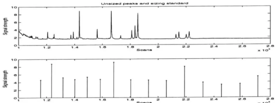
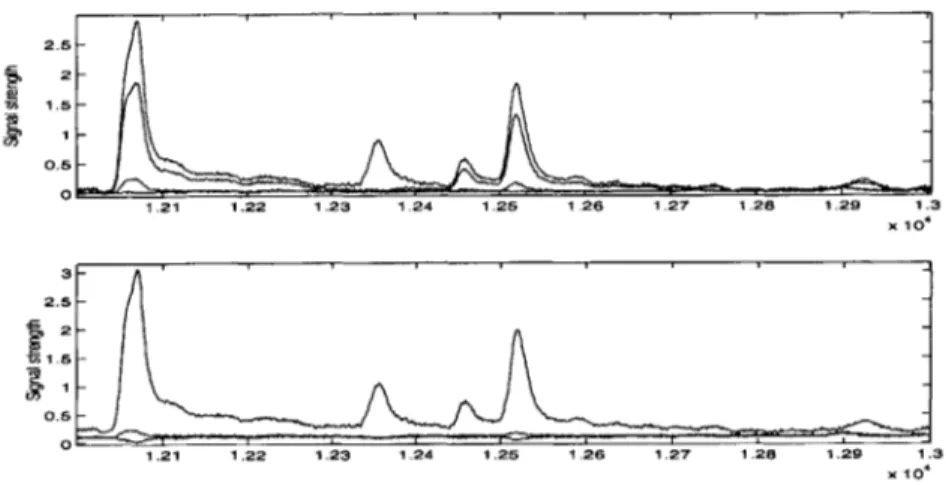
To determine absolute sizes, a collection of molecular weight markers, known as an internal lane standard, is loaded onto the separation electrophoresis along with the samples. Because the internal lane standard sizes are known, comparing the migration times of the unknown alleles against the standard's yields their sizes. See Figure 3-2.

- Original double-siranded DNA 51

I

New pdirieru -w \rc%.t%.r4rJNrttrk~1

Figure 3-1: A general view of the PCR process. Primers attach to both strands of

DNA at the 3' end. Replication occurs from the primers out towards the 5' end. Since

a single strand of DNA is replicated into two strands, the number of replications is roughly exponential base 2 to the thermal cycle. Source: National Human Genome

Research Institute.

3.1

Demred Iugirnrt

Figure 3-2: Time profile expressed as voltage versus time in scans. The peaks in the top panel correspond to unsized fragments that must be sized relative to the standard peaks on the bottom panel.

3.4

Allele Calling

Once the fragments have been sized, they must be identified. Unfortunately, identifi-cation, or allele calling, is nontrivial since the allele sizes of different genetic markers may overlap. Another source of confusion is the behavior of the PCR kits: Recall that different kits yield different fragment sizes for the same genetic marker. Thus, accurate allele calling necessitates taking the kit used for PCR into account.

3.5

Profiling

With the sample profile in hand, forensic investigators can compare it against a database of criminal profiles (such as CODIS). Because of the extremely low average random match probability, a match between a sample and criminal profile positively traces the sample as coming from the profiled individual.

nsi-a P-ke almima atmn -O

10

Z.8

10

0 1 I.A

Chapter 4

Automated DNA Typing Systems

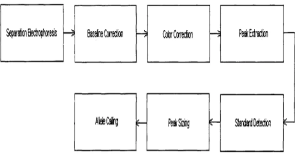
As DNA genotyping technology continues to evolve, a need has grown for faster and more efficient throughput to match advances in hardware. The development of au-tomated DNA typing systems is a response to that need. Auau-tomated systems boast improved throughput and time-savings through parallelism and rapid analysis. The bulk of research in developing automated systems focus on replacing manual depen-dencies in the signal-analysis stages of separation electrophoresis and allele calling (Figure 4-1).

4.1

Automated DNA Separation Electrophoresis

Automated DNA typing systems typically run multiple separation electrophoresis in parallel. Representative systems, including the variant system in our lab, boast

16-384 parallel lanes for multiple, simultaneous experiments.

Each lane is pre-loaded with a polyacrylamide gel matrix that serves as the molec-ular sieve. Lanes may be preferentially loaded to improve base pair resolution. The fragments are labelled beforehand with fluorescent dyes to help detection when they exit the lane. The number of dyes employed depend on the particular system and the kit involved. A typical system employs four dye colors to differentiate between frag-ments and reserve an additional fifth color for the internal lane standard. A scanning laser at the exit end of the matrix excites the dyes as the fragments pass through. The

A9,Pei

Stg

Rak

~do

Figure 4-1: The signal processing stages involved in an automated DNA typing sys-tem, from separation electrophoresis through allele calling.

excitation causes a measurable fluorescence that is captured by an optical system (for example, photomultiplier tubes) and converted to a voltage signal. The end result is a collection of lane profiles expressed as voltages against time in scans.

Ideally, signal peaks in the lane profile correspond to times when a collection of similarly sized fragments exit a lane. Because the standard and unknown fragments are separately labelled, their respective peaks are easily distinguished from each other. Hence, one can ascertain the allele sizes by comparing the relative positions of their signal peaks against the standard.

Unfortunately, noise sources significantly complicate the process outlined above. Before fragments can be properly sized, the lane profiles must undergo multiple signal processing passes to resolve actual data from noise.

4.1.1

Baselining

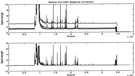
Generally, the first signal processing stage involves smoothing out the baseline in a lane profile. The sensitivity of the optical filters, small fluctuations in the voltage gradient, and natural fluorescence in the surrounding environment all contribute to an uneven baseline in the lane profile. Additionally, color channel bleed-through can elevate the baseline. (See 4.1.2). Uneven baselines are undesirable because they

I

Before and After Baseline Correction 10 B- 6- 4-2 _L 00 0.5 1 1.5 2 2.5 3 3.5 4 Scans X 104 a 6- 4 -0 0.5 1 1.5 2 2.5 3 3.5 4 Scans X 104

Figure 4-2: An example lane profile before and after baseline correction. Notice that artificially elevated and uneven baselines have been normalized.

hinder accurate assessments of signal strength: The weaker of two signal peaks may nonetheless be stronger overall because it conveniently sits on at a higher baseline than the other. (Figure 4-2). Because later signal processing stages make use of signal strength, a flat baseline contributes to an accurate lane profile analysis.

4.1.2

Color Correction

The PCR reaction is usually multiplexed so that multiple target STR markers are amplified in parallel. Multiple fluorescent dye colors are used to distinguish between alleles belonging to different markers with overlapping size ranges. The number of dyes used varies depending on the parameters of the experiment. As mentioned above, a typical, multiplexed system involves the use of four different dye channels for the samples, with a fifth reserved for the standard.

The waveform spectra of the dyes overlap to some degree. This leads to a bleed-through effect where peaks in one color channel artificially elevate the baseline of another. Peaks may also erroneously appear in the wrong color channel.

Bleed-through effects can be modelled as the convolution of one color channel with another. Hence, one can form a convolution matrix that parameterizes the contributions of each channel on the others. Color-correction algorithms generally

2.52 -. 1.5- 0.5-1.21 1.22 1.23 1.24 1.25 1.26 1.27 1.28 1.29 1.3 10 1.21 1.22 1.23 1.24 1.25 1.26 1.27 1.28 1.29 1.3 X104

Figure 4-3: An example lane profile before and after color correction. Note that there is significantly fewer "bleed-through" peaks after color correction. Additionally, signal strength changes as both positive and negative contributions of the bleed-through are eliminated.

employ the inverse matrix

(known

as a color correction matrix) to ameliorate the bleed-through effects in each channel. When the spectra of the dyes are known beforehand, the color correction matrix can be calculated prior to the experiment. When the spectra are unknown, the color correction matrix must be dynamically generated based on the lane profile and channel information.[3] Figure 4-3 gives an example of color correction.

4.1.3

Peak picking

Signal peaks within a lane profile represent instances where fragments of similar sizes exit the lane. Because they represent fragments of a certain size, signal peaks are com-pared against internal lane standard peaks when sizing the fragments. Consequently, properly identifying and selecting them from a lane profile is important.

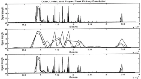
Unfortunately, the choice of resolution complicates this task. If the resolution is too low, neighboring peaks may be misidentified as one large and broad peak. Conversely, if the resolution is too high, one large and broad peak may be misidentified as many smaller peaks. See Figure 4-4.

Over, Under, and Proper Peak Picking Resolution 6-S4 2 0 0.5 1 1.5 2 2.5 3 3.5 x Scans Xl 86 - 4c 2 -S 0.5 1.5 2 2.5 3 3.5 4 Scans X 10 4

Figure 4-4: An example lane profile with over, under, and proper peak picking res-olution. Over resolution leads to numerous peaks being picked, with a subsequent decrease in computational efficiency. Under resolution leads to very few peaks being picked and reduces accuracy. A proper resolution allows for acceptable computation efficiency and accuracy. Appropriate resolutions depend on the scanning frequencies used to generate the lane profiles, as well as the fragment sizes of the experiment.

into windows of a given size and determining the local maximum in each window. If the maximum is centered then it qualifies as a peak. The choice of window size determines the peak-picking resolution.

4.1.4

Stutter Correction

During PCR, an occasional miscopying may lead to a shorter duplicate than the original. The miscopying stems from slippage in the copying mechanism. Although infrequent, the sheer number of copying involved in PCR means that such slippage artifacts have a noticeable effect on the lane profile.

Slippage artifacts are represented in a lane profile as short, "stutter" peaks that are very close to the actual peak. Stutter peaks complicate peak picking, and by ex-tension, allele calling: Given two peaks positioned closely together, it may be difficult to determine whether they are two legitimately separate peaks or whether one is a

stutter peak of the other.

convolu-Standard Comparisons In 2 Experiments 21.5 -0.5 --0.8 1 1.2 1.4 1.6 1.8s 2 2.2 2.4 2.6 2 2.5- i i i i i 2-1.5 --0 .5 0.8 1 1.2 1.4 1.6 1.8 2 2.2 2.4 2.6 2.8 Scans X 10

Figure 4-5: Channel profiles of the same standard in two experiments. Note the dramatic disparity in scan positions and signal strength.

tion of a noise source and an actual signal. Assuming known convolution parameters, performing the inverse operation removes the stuttering effects. Stutter correction algorithms generally employ this strategy. To determine the convolution parameters, such algorithms require a noiseless

lane

profile to reference.

4.1.5

Standard Detection

The process of identifying and selecting the internal lane standard peaks from a lane profile subtly differs from peak picking. Peak picking identifies and selects all peaks

in sample color channels of a lane profile. Standard detection, on the other hand,

identifies and selects a specific set of peaks in one color channel of the lane profile. As

with peak picking, selecting a proper resolution is important. Additionally, however, standard detection must contend with differentiating between actual standard peaks and noise.

Noise peaks may come from impurities in the standard and lane and color channel

variations. The problem is exacerbated in that the same internal lane standard may have very different peaks across experiments. Variations in sampling frequency and cutoff times dramatically alter the standard peaks in a lane profile. Figure 4-5.

4.2

Automated Allele Calling

Identifying fragments requires referencing their sizes against an allelic ladder. An allelic ladder is a collection of alleles with known size ranges. In principle, the frag-ments' identities are precisely the alleles that best match their sizes.

The situation is more complicated in practice. The allelic ladder is based on the PCR kit and fragment sizes may vary even when the same kit is used across experiments. While kits contain documentation with expected size ranges for the alleles, the ranges overlap since certain alleles may differ by a single base.

When identifying similarly-sized fragments, it can be difficult to tell if they are different alleles with overlapping size ranges or are instances of the same allele. Even identifying one fragment can provide a challenge if its size fall within overlapping ranges for two alleles.

Chapter 5

Thesis Topics

This document presents algorithmic solutions to the standard detection and allele call-ing problem in an automated DNA typcall-ing system. For each half, it starts by delvcall-ing into a deeper description of the problem. It then walks through the algorithms' solu-tion processes before presenting them in a general overview. Experimental evidence demonstrating their correctness and effectiveness is provided along with analysis of their running times and requirements. Each half ends with suggestions for future improvements and expansions.

5.1

Automated Standard Detection

5.1.1

The Problem

Differentiating between standard and noise peaks is a significant problem. Poor color correction and impurities within the lane can lead to many false peaks in the lane profile. Preferential loading exacerbates the problem since it causes peak height to vary and may lead to some noise peaks being stronger than actual ones. Signal-to-noise ratio drastically fluctuates as a result and signal strength alone is consequently unreliable as a noise determinant.

The lane profile for the same standard fluctuates between experiments. The com-bined effects of the scanning frequency and cutoff times can shift, clip, and scale the

Peak Spacings versus Sizes 1400 1200- 1000- 1800-&600 400- 200-0O -- - - - _ _ _-0 80 100 120 140 160 180 200 225 250 275 300 325 350 375 Standard sizes (in base pairs)

Figure 5-1: Peak spacings plotted as a function of .the peak sizes for sizes between

80 and 400 bp. For example, the spacing between the 80 and 100 bp peak is around 800 scans while that between the 375 and 400 bp peak is around 1200 scans. Notice

that as peak size increases, the spacing between the peaks increases even if the size difference remains the same. Observe the change in spacing from around 800 scans

(for the 100 and 120 bp peaks) to 950 (for the 180 and 200 bp peaks).

standard peaks in both time and signal strength. (Refer back to Figure 4-5). Static descriptions of the standard peaks therefore fail as a determinant as well.

Finally, the distances between standard peaks is nonlinear to the corresponding differences in standard fragment sizes. As shown in Figure 5-1, the spacing between the 80 and 100 base pairs peak is significantly less than that between the 180 and 200 base pairs peak-even though the difference between both sets of peaks is 20 base pairs.

These factors combined make it very difficult to filter out noise by traditional means. A novel algorithm is required to differentiate standard peaks from noise.

5.1.2

The Solution Process

A Comparison Metric

Differentiating standard peaks from noise implies applying some sort of metric to evaluate different peaks. Ideally, high-scoring peaks will correspond to the standard

1.6- 1.4-

1.2-

0.8,-s0 80 100 120 140 160 180 200 225 250 275 300 325 350 375 400 Fragment size (in base pairs)

x 10

2.5-

2-0.51

50 80 10 120 140 160 180 200 225 250 275 300 325 350 375 400 Fragment size (in base pairs)

Figure 5-2: Plots of peak positions versus fragment sizes. The top panel, (a), plots the relationship for one standard in experiment. The bottom panel, (b), plots the relationship for the same standard in two experiments. Notice that the behavior of the standard is varies across different experiments. No single, parameterized model can capture the general behavior of the standard.

The lane profile provides information on the position and signal strength of stan-dard and noise peaks. Any comparison metric must use either or both sets of in-formation. Because signal-to-noise ratio varies so dramatically, signal strength is marginally useful. Therefore, the comparison metric relies primarily on peak position information.

Recall that shorter fragments yield signal peaks earlier in the lane profile than longer ones; Peak position and fragment size are causally related. Figure 5-2a shows a plot of the relationship for one standard in an experiment.

From the figure, it is tempting to try and model the relationship by a second order function, p =

f(s)

= qs2

₊

rs + c where p denotes peak position, s denote fragment

size, and q, r and c are coefficients. Such a model can predict the standard peak positions in any experiment if the coefficients are known. Unfortunately, the model has a fundamental flaw:

q, r and c encapsulates the shifting, scaling, and clipping effects of the scanning

frequency and cutoff times: q and r are related to the potential gradient applied during the separation electrophoresis and the composition of the gel matrix. This

differs from experiment to experiment and even from lane to lane. c reflects the offset from the 0th scan position of the peaks in the profile, which again, differs with each experiment. So the coefficients cannot be reliably determined beforehand.

The only way to determine the coefficients is to estimate them from a few standard peaks. In other words, one must first find a few of the standard peaks in a lane profile and estimate the coefficients from there. With the estimations in hand, the model can be used to discover the remainder of the standard peaks in that lane profile. Unfortunately, finding any number of the standard peaks is on the same order of difficulty as finding all the standard peaks. Hence, very little is gained from this approach. Moreover, the coefficients must be re-estimated with each new lane profile as the behavior of peak positions versus fragment sizes varies across experiments. (See Figure 5-2b).

Rather than a second-order model, a better approach involves partitioning the data and fitting each partition into a local, linear model. On a small scale, the relationship between fragment size and peak position is linear. (Figure 5-3). By

accepting piecewise linearity, the relationship between peak position and fragment size becomes: p = f(s) = qs + c. For any two neighboring peaks, pi and P2, it must

be the case that pi = qsi + c, and P2 = qs 2 + c. So, P2 - Pi = q(s2 - Si).

Finding the proportionality coefficient, q, for each partition runs into the same problems encountered by the second-order model. Fortunately, q can be factored

away if each piecewise partition contains at least three peaks.

For any three neighboring peaks in the same partition, P1,P2,P3, it must be the

case that P2 - Pi = _q(82 - Si) and P3 - P2 = q(s3 - 8₂). Therefore, P -P =2- 2 We

can rewrite this as: -_

/

-= 1.

This leads to a natural comparison metric: Given three neighboring peaks P =

{Pk > pj > pi} and sizes S = {sk > sj > si}, define the ratio R(P, S) PkP/ 8 k-.

When Pk, pj, and pi are the peaks of the respective standard fragment sizes, R is

exactly 1.

This important result yields a workable model of the relationship between peak positions and fragment sizes.

X 10, Fragment Sizes versus Peak Positions 21.6 1.4 - S1.2- 1-50 80 10 120 140 160 180 200 225 250 275 300 325 350 375 400 Fragment size (in base pairs)

X 10,

G 1.8 1.4 S1.2

-~~ ~

~

Fragment size (in basspairs) 30 30 40

Figure 5-3: Plots of peak positions versus fragment sizes. The top panel, (a), plots the overall relationship between peak position and fragment size. The bottom panel,

(b), plots the local relationship for the same standard. Notice that as opposed to the

global level, on a local level, the relationship is approximately linear.

A Scoring Function

The comparison metric, while a good start, does not suffice alone to differentiate between signal and noise peaks. There are two major problems.

First, while the metric predicts a standard peak spacing-to-size ratio of exactly

1, actual ratios fluctuate around 1 (usually around 5%, or between 0.95 and 1.05).

Given R1 = 0.97 and R2 = 1.05, the comparison metric does not say which is more

desirable. Secondly, the metric does not help to differentiate between standard peaks and noise peaks that happen to have a high Rnoise. Indeed, it may even prefer noise peaks over standard ones if Rnoise happens to be exactly 1. See top panel of Figure 5-4.

Both problems can be rectified by introducing a suitable scoring function on top of the comparison metric. To that end, let's define the scoring function, S(P, S) where

P is a triplet of peaks and S is a triplet of sizes.

To address the first problem, tentatively define S(P, S) as S(P, S) = min(R(P, S), 1/R(P, S)). Doing so guarantees that S(P, S) measures the deviation of the ratios

R(P, S) for several standard peak triplets 1.4

p3 p4 pI pI p p8 p p 1I

I

T

Standard peak triplets

Deviation of R(P. S) from 1 for several standard peak triplets

p12 p13

p5 p6 p7 p8 p9

Standard peak triplets plO p11 p12 p13

Figure 5-4: (Top) The ratio R(P, S) for various triplets of standard peaks. Notice that the ratio fluctuates around 1, with some values being as high as 1.3. When the values are significantly off from 1, noise peaks may supplant some of the actual ones if Rnoise happens to be closer to 1. (Bottom) A measure of the deviation of R(P, S) from 1, for the same set of standard peak triplets.

1.3 1.2 cc1. 0.9 -0.8 p1 p2 0.95 0.9

Ir

0.85

T

T

L > < 0.8 0.75 p1 p2 p3 p4 7

'

1 0.

function will value R1 over R2 since the deviation of R1 from 1 is less than that of R2

from 1. See bottom panel of Figure 5-4.

To address the second problem, we make the following observation: Let P, =

{pi

<

P2 < P3} and P2 = {P2 < P3 < p4}. Suppose R(P2, S2) = 1 for S2 = {s2 < S3 < S4}.

Then there must be an Si = {si < s2 < S₃} such that R(P, Sj) = 1. The insight here

is that a set of positions is correct if and only if some earlier set is correct (unless, of course, it is the first correct set). The reasoning is reminiscent of induction. Under this constraint, noise peaks will have difficult achieving high scores.

Capturing this notion into the scoring function involves a simple refinement to its definition. Let P be a triplet pi < Pj < Pk, S be a triplet si < s3 < sk, and R be

the computed ratio. Then S(P, S) = max({S(P', S')})xmin(R, 1/R) where P' is a

triplet Ph < pi < pj and S' is a triplet Sh < Si < sj.

The scoring function essentially estimates the likelihood that a given triplet of peaks is a triplet of standard peaks.

Scoring Table

A scoring table maintains scores between peak positions and sizes. Row indices

cor-respond to triplets of standard fragment sizes. Column indices corcor-respond to triplets of peak positions in the lane profile. Both row and column indices are organized in increasing lexicographic order. An entry in the table is the score of the intersecting row and column indices. See top panel of Figure 5-5.

The row indices are computed as follows: For every size si excepting the largest two, a triplet is formed with sizes s2 and s3, where S2 is the least upper bound of s1,

excluding itself, and s3 is the least upper bound of S2, excluding itself. The set of

these triplets will cover the range of all the sizes in the standard ladder. See middle panel of Figure 5-5.

The column indices are computed as follows: For every three positions, pi < p, <

Scoring Tabte of Standard Frazgment Sizes and Peak Pacitions PI P. . PY 54--. F 5S P! S .t Standard Sizes ts-, s ss s. s . s (ss; - 5 s , S (5 4 -1 S . . S w+ Z PE-4KS Positk-ns4 -- 6' CpP-*' I. P.P -- PO P (P,, P , Ps PL where n = k choose 3

(p Ip.J

p 1J. p s p p ip P .p ). (p I pt p (pI, p-4, p! (p ppJ. (p-l P A p-:p).

Figure 5-5: The scoring table. (Top) General structure. (Middle) Computing the row indices. (Bottom) Computing the column indices.

S f S f2 Sf3 Sf4 Sf5 f6 Sf7 Sf8 9 5f

o

Sg

Sg2

Sg3

Examined entries

Top scoring entry examined for that row * Starting position for that row

Figure 5-6: An example of a backtracking path. The algorithm starts in the rightmost, bottommost cell and works its way diagonally left to the top row.

Backtracking

The scoring table, when completed, provides the scores between every pair of peak position and standard size triplets. Differentiating between the standard and noise

peaks then involves searching through the table for the highest scoring entries that

represent the standard peaks.

The search involves backtracking through the table, starting from the rightmost

entry of the bottom row and ending at the top row.

For each row i, (excepting the bottom row) the backtracking algorithm finds the

highest-scoring entry, Sj(P', S'), to the left of the starting position in that row. It

then compares Si(P', S') to the highest-scoring, recorded entry, Sj+1(P, S), from the

previous row. If P' = Ph < pi < p, and P = pi < p, < Pk then Si is recorded and

the algorithm moves up to the ith - 1 row from Si's column position. Otherwise,

the algorithm discards Si and searches for the next highest-scoring entry to compare

against Si+1 .

For the bottom row, the backtracking algorithm simply finds and records the

highest-scoring entry before moving up a row from the entry's column position. See

Figure 5-6.

When the backtracking algorithm has recorded the entry for the top row, it returns

the union of the Pi's from its records. The returned set corresponds to the positions of the standard peaks in the lane profile.

5.1.3

Search Algorithm

General Overview

The fundamental idea behind the algorithm involves reducing the problem of differen-tiating between standard and noise peaks into the simpler one of substring matching. Briefly, the substring matching problem asks to find the best match between a source string and a target string. For example, if the source string is ATTTGACAC and the target string is TTGC, the best matching substring is ATTTGACAC.

Here, the algorithm attempts to match the "substring" of standard fragment sizes against the "substring" of peak positions in the lane profile. Rather than using the equivalence relation as a scoring metric (as per normal substring matching), the algorithm employs the scoring function, S(P, S).

The construction of the scoring table is analogous to the ones used in dynamic programming solutions to the substring matching problem. The primary difference is that the "letters" of the substrings are really triplets of numerical values.

Once the table is completely filled in, the backtracking algorithm searches through the table and returns the positions of the standard peaks in the lane profile. As with substring matching, the backtracking algorithm works on a dynamic programming paradigm.

An Illustrative Example

The following simple example illustrates the various steps of the algorithm. Suppose the following lane profile: (0.8v, 1 scans), (1.0v, 2 scans), (0.5v, 4 scans), (0.9v, 7

scans), (0.65v, 10 scans), (0.8v, 20 scans) where the left point of the pair represents signal strength in voltage and the right point of the pair represents the time (in scans) where the peak appears in the lane profile. See top panel of Figure 5-7.

A sample lane profile. internal lane standard, and corresponding peaks

04AA

A,

0 > 5 10 5 20 Scans (x 104) 0 50 100 150 200 250 300

Standard fragment sizes

0 0 1 0 25

Scans (x 104)

Figure 5-7: (Top) An example lane profile. (Middle) An example internal lane stan-dard. (Bottom) The peaks in the example lane profile that corresponds to the internal lane standard.

bp. See middle panel of Figure 5-7. The algorithm will now determine the standard

peaks in the lane profile.

It starts by constructing the sets of triplets of peak positions and sizes. spositions = _{(1, 2, 4), (1, 2, 7), (1, 2, 10), (1, 2, 20), (1, 4, 7), (1, 4, 10), (1, 4, 20), (1, 7, 10),}

(1, 7, 20), (1, 10, 20), (2, 4, 7), (2, 4, 10), (2, 4, 20), (2, 7, 10), (2, 7, 20), (2, 10, 20),

(4, 7, 10), (4, 7, 20), (4, 10, 20), (7, 10, 20). Sizes = (80, 100, 200), (100, 200, 260).

In the next step, the algorithm constructs and completes the scoring table, using

the elements of SpOstj,, and Sizes as column and row indices, respectively.

(1,2,4) (1,2,7) .. . (2,7,10) ... (7,10,20) (80,100,200) 2 1 ... 3 2

(100,200,260)

-

6 ... ...

The backtracking algorithm searches through the completed table and returns the peak positions 1, 2, 7, 10. These elements correspond with the peaks (0.8v, 1 scan), (1.Ov, 2 scans), (0.9v, 7 scans), and (0.65v, 10 scans) in the lane profile. They are the best candidates for the standard peaks. See bottom panel of Figure 5-7.

5.1.4

Analysis and Conclusion

Validation

42 different lane profiles were used to validate the algorithm. Of the 42 profiles,

32 contained internal lane standard peaks and 10 did not. The same internal lane

standard was used for all 32 profiles. Determining the algorithm's correctness involved comparing the results against a gold standard: Namely, a manual determination of the standard peaks in a lane profile by an experienced technician.

The algorithm correctly identified the standard peaks in 30 of the 32 and correctly determined that the standard peaks did not exist in 10 of the 10. In the two cases where the algorithm failed, the algorithm incorrectly selected a noise peak that was within a few scans of the one selected by the gold standard.

10 artificial lane profiles (each containing a different, fabricated internal lane

stan-dard) provided additional validation to ensure the algorithm did not overfit the orig-inal set of 42. In all 10 cases, the algorithm correctly determined the peaks that corresponded to the fabricated standard.

The encouraging performance of the algorithm on the validation sets (50/52 cor-rect, 2/52 incorrect), suggests it is accurate enough for use in automated DNA geno-typing systems.

Failure Analysis

In the two cases where the algorithm incorrectly identified the standard peaks, it selected a noise peak within a few scan units of the actual one. The error stems directly from the definition of the scoring function, S(P, S).

The definition of S(P, S) makes it very difficult for a sequence of noise peaks to masquerade as standard ones. However, it does allow an occasional outlier peak to replace an actual one if they happen to be close neighbors.

Suppose P' = Pnoise < Pstandard2 < Pstandard3 and P" = Pstandardl < Pstandard2 < Pstandard3. Owing to the fact that the linear model is, after all, an approximation, if

Superficially, this represents a serious flaw in the scoring function. However, the actual effect is minimal since peak positions are usually on the order of several thou-sands of scan units. A deviation of a few scan units translate to a very low percentage difference and does not significantly affect accuracy when using the internal lane stan-dard to size the fragments.

Running Time and Space Analysis

Given a channel profile with JP number of peaks and a standard ladder with |SI sizes, the algorithm takes

1S1

- 2 computations to find the row indices of the scoring table and JPI choose 3 computations to find the column ones. Hence, the total time needed to reduce into substring matching is O(IS1 + P 3).

Both filling in, and backtracking through, the table requires O( Sl|plj3). Hence, the total running time of the algorithm is: O(ISP Ip1) + O(ISIIPI3) + O(SI+ I P13) or

simply

0(SIIP1

3

_).

In comparison, a brute force approach would need to compute each substring of size ISI in the data set and score it against the model. There are lPIchooseSI such substrings. Hence, computing the substrings alone would take 0((LL)ISI) time.

To compare all the substrings against the model would then take 0(

jpJ!)

time. Hence, the total running time needed is: 0(

jP1').

For P >> S and S > 3, the algorithm performs exponentially better than brute force. The number of sizes in the standard ladder is typically many times smaller than the number of peaks in a channel profile, and also usually contain more than three fragments. The algorithm is therefore useful in most practical cases.

5.1.5

Future Extensions

While the algorithm works very well for lane profiles with a small to moderate number of peaks, the algorithm slows dramatically when processing many peaks.

Because the algorithm runs in cubic time and space with the number of peaks, a tenfold increase in peak number translates to a thousand-fold increase in running

time and space. Of the two, the space requirement is more problematic. Processing capabilities of modern computers can easily handle the algorithm's time demands; On the other hand, memory remains limited and expensive.

Empirical evidence has shown that running the algorithm on a lane profile with several hundred peaks requires more memory than physically available on the current genotyping system. This is the primary cause of the dramatic slowdown as the system is forced to read from, and write to long-term storage in addition to the cache.

Any improvement in the space requirement of the algorithm will significantly improve its utility. One possible research direction is to overlay a divide-and-conquer approach on top of the algorithm. Namely, divide the lane profile into discrete, overlapping frames, run the algorithm on each frame, and reconstitute the general solution by finding the union of the individual frame solutions. While the divide-and-conquer approach may increase running time requirements, the increase is offset by the reduction in the space requirement.

Another potential improvement involves increasing the amount of information used by the algorithm. The algorithm currently uses only peak position and fragment sizes as parameters into the scoring function. While this is sufficient for internal lane standard detection, it may be inadequate for other applications. Because of its generality, the possibility exists that the same algorithm may be used to ameliorate signal processing issues in similar technologies (such as DNA sequencing).

In such applications, signal strength and duration may be equally valid parameters for differentiating between noise and signal. Hence, extending the algorithm to work in multiple feature spaces may be desirable.

5.2

Automated Allele Lookup

5.2.1

The Problem

Matching sized fragments to the entries in an allelic ladder presents a difficult chal-lenge. One or more fragment sizes may fall within overlapping ranges of multiple

Allele sizes for one genetic marker 145 U 140-135 -2 B 130-A 125 120 Al A2 A3 AA A5 A6

Alleles for one genetic marker

Figure 5-8: (A) A fragment size here will fall into overlapping allele ranges. (B) A fragment size here falls outside of all allele ranges.

ladder entries, in which case proper registration becomes problematic. Conversely, a fragment size may fall outside of the ranges of every entry in the ladder, in which case one must decide whether it is a proper allele or residual noise. See Figure 5-8A and B. Even small sizing errors of one or two base pairs become significant as certain allele sizes differ by as little as a single base pair.

The simplistic approach of registering each sized fragment to the closest matching entry in the allelic ladder fails to consistently give a correct result. Consider the following example: Suppose sized fragment of 150, 160, and 162 base pairs and allelic ladder entries of 148, 158, 160, 165 base pairs. Each entry has a +/- 1 base pair range. The naive approach incorrectly gives the registered pairs 150-148, 160-160, and 162-160 base pairs. The correct registration, as given by a gold standard, is 150-148, 160-158, 160-162 bp. Finding the optimal registration requires using additional information, such as the ranges for each entry, that is ignored in an uninformed search. As a result, proper registration via blind searches is difficult. A more sophisticated search algorithm is needed to reliably find the best matches between sized fragment and the allelic ladder.

Registration error using S.S.E. for S = (x, x2), M = (yl, y2)

200- .

---10 - -

-1 2 .... .... -- -1

100--

-Figure 5-9: The registration error according to an S.S.E. objective function for two-dimensional vectors

S

=

(xi, x

₂

)

and M =

(yi,

y2), over various deviations of y, from

xi. Notice that under the S.S.E., minimal registration error occurs when S and M are identical (i.e. perfectly aligned).

5.2.2

The Solution Process

Objective Function

Finding the best matches suggests searching for the combination that minimizes reg-istration error. The ideal regreg-istration error decreases as the algorithm approaches the optimal matches and increases as it wanders away.

Borrowing from image registration theory, the algorithm employs an objective function based on the Summed Square Estimation (S.S.E.) to quantify the registration error. Briefly, given two vectors S = (..,x 2, ...,x) and M = (y, y2, ... , y), the error

is determined by (x1 - y1)2 + (x2 - y2)

2 ₊

... + (x, - ya)2 _{and is a measure of the} degree to which they deviate from each other. See Figure 5-9.

Here, the objective function is quantifying the registration error between the sets of fragment and allelic ladder sizes. Because of the squaring, the S.S.E. accentuates errors and allows for fine-grain resolution. Good error resolution is important in this case as allelic ladder sizes may differ by as little as a single base pair.

Confidence Measure

While useful, the S.S.E., (and consequently the unmodified objective function), in-correctly quantifies the registration error between fragment and ladder sizes in many cases.

Under the S.S.E., registration error is minimized when fragment size are matched to the closest allelic ladder sizes. Unfortunately, this is not always desirable or correct. Consider the following example: Suppose fragment size x1 = 120 bp and allelic ladder sizes Y1, Y2 = 117 and 122 base pairs, respectively. Further suppose that yi has a size range of +/- 2 base pairs and Y2 has a size range of +/- 1 base pairs. The S.S.E. gives a minimum registration error when x1 is matched to Y2. However, x1 falls outside

of the size range for Y2, but inside the range of yi. Hence, registration error should actually be higher for Y2 than yi. The S.S.E. yields an incorrect result because it does not take size ranges into account when computing the registration error.

Clearly, the objective function must be modified to take size ranges into consid-eration. In particular, when the fragment size does not fall into the ladder entry's size range, the registration error must increase. When it does, the registration error should remain the same as before.

Adding confidence measures to the objective function fixes the shortcoming. For two vectors, S = (X1, x2, ..., Xn) and M = (yi, Y2, ..., yn, the modified objective func-tion computes the registrafunc-tion error as a weighted Euclidean distance. Namely, the error is determined as a,(xi - yl)2 _{+ a}

2(x2 - Y2) 2 + ...

+

an(x, - yn)2, where the ai's are the confidence measures for the corresponding matches between the xi's and yi's. For any i, when xi falls within the size range for yi, a, is 1. So the contribution to the registration error for the pair remains unchanged. When xi falls outside the size range for yi, ai is equal to 1 + the distance between xi and the closest border of

yi. For example, when xi = 110 base pairs and y, = 112 base pairs with a range of

+/- 1 base pairs, ai = 1 + (111 - 100) = 2. As the example illustrates, the extra + 1 term is important as otherwise a, = 1.

~ium -. -

-Registration error using confidence measures for S = (xl, x2), M = (yly2)

10..-0-1

40--a2(x2 -y2) - - al(x1 - yl)

Figure 5-10: The registration error according to the modified objective function using confidence measures. S = (xi, x2) and M = (Yi, y2), over various deviations of y.

from xi. x1 and x2 both have a range of

+/-

1 in this situation. Generally, different

alleles have different size ranges.

grows much quicker than that for the S.S.E. as x, moves out of the range of ye. This translates to much tighter bounds on acceptable matches for low registration errors.

Notice that even with the confidence measure, the objective function may still compute a lower registration error for a match where x, lies outside the range of ya. Consider the case where x1 = 110 base pairs, yi = 112 base pairs with a range of

+~/- 1 base pairs, and y2 = 113 base pairs with a range of

+/-

3 base pairs. In this

instance, the modified objective function gives a registration error of 8 for (xi, yi) and an error of 9 for (xi, y2).

The problem stems from the fact that y2 and its size range completely encompasses yi and its range. Such situations, while theoretically possible, are uncommon in everyday practice. While the ranges may overlap for various allelic ladder sizes, they do not encompass one another. This is an intrinsic property of the PCR kits used to determine the allelic ladder. Hence, the modified objective function performs correctly under everyday situations.

Dynamic Programming

The objective function clearly shows that the registration error contributions of each

(Xi, Yi) pair is independent of the others. This suggests that the minimum registration error between the entire vectors (Xi, x2, ... , Xn) and (yi, Y2, ... , yn) occurs when the error

contribution of each (xi, yi) pair is minimized; when each of the xi's are matched to the best candidate yi.

This is a classic example of an optimal solution to a subproblem leading to an optimal solution for the global problem. The principle of dynamic programming is therefore applicable. To find the best matches between fragment and allelic ladder sizes, the algorithm simply finds the best-matching ladder size for each fragment size and forms the composite set out of all the pairs.

Note that the dynamic programming principle applies in this case because of the choice of objective function used to quantify the registration error. A different objective function may very well invalidate application of the principle.

Search Methodology

Finding the best match between fragment and allelic ladder sizes requires comparing candidate matches against one another and searching for the best ones. The algorithm models the process as a heuristic-guided path search where it tries to find the optimal path from an initial state to an unknown goal state.

The initial state is defined as the state where all the fragment sizes are unmatched. The goal state is defined as the state where all the fragment sizes are matched. Intermediate states may have any number of matched fragment sizes.

A state in the model is a set of fragment sizes. Each fragment size is labeled as

matched or unmatched. When a fragment size is matched, the matching ladder size is included as part of the state description.

A state transitions to another by matching an unmatched fragment size to a

ladder size. To limit the number of possible transitions, the algorithm only examines transitions that match the smallest, unmatched fragment size. Such a constraint