Algorithms for Reconstruction of hidden 3D shapes using diffused reflections

Algorithms for Reconstruction of hidden 3D ARCHIVES

shapes using diffused reflections

by

_j

Otkrist Gupta

B.Tech. in Computer Science and Engineering, Indian Institute of

Technology Delhi, 2009

Submitted to the Program in Media Arts and Sciences,

School of Architecture and Planning

in partial fulfillment of the requirements for the degree of

Master of Science in Media Arts and Sciences

at the

MASSACHUSETTS INSTITUTE OF TECHNOLOGY

June 2012

@

Massachusetts Institute of Technology 2012. All rights reserved.

Author ...

...

Program in Media Arts and Sciences,

Sool of Architecture and Planning

May

07, 2012

Certified by...

Ramesh Raskar

Associate Professor of Media Arts and Sciences,

Program in Media Arts and Sciences

Thesis Supervisor

Accepted by ...

...

...

Mitchel Resnick

LEGO Papert Professor of Learning Research,

Academic Head,

Program in Media Arts and Sciences

Algorithms for Reconstruction of hidden 3D shapes using

diffused reflections

by

Otkrist Gupta

Submitted to the Program in Media Arts and Sciences, School of Architecture and Planning

on May 07, 2012, in partial fulfillment of the requirements for the degree of

Master of Science in Media Arts and Sciences

Abstract

This thesis aims at discovering algorithms to recover the geometry of hidden objects

from tertiary diffuse scattering, given time of flight information. We focus on using

ultra high speed capture of photons to accurately determine information about dis-tance light travelled and using it to infer hidden geometry. We aim at investigating issues such as the feasibility, uniqueness(in solution domain) and invertibility of this problem. We also aim at formulating the forward and inverse theory of secondary and tertiary diffuse scattering using ideas from tomography. We aim at developing tomography based approaches and sparsity based methods to recover 3D shapes of objects "around the corner". We analyze multi-bounce propagation of light in an unknown hidden volume and demonstrate that the reflected light contains sufficient information to recover the 3D structure of the hidden scene. We formulate the for-ward and inverse theory of secondary and tertiary scattering reflection using ideas from energy front propagation and tomography. We show that using careful choice of approximations, such as Fresnel approximation, greatly simplifies this problem and the inversion can be achieved via a backpropagation process. We provide a theoreti-cal analysis of the invertibility, uniqueness and choices of space-time-angle dimensions using synthetic examples. We show that a 2D streak camera can be used to discover and reconstruct hidden geometry. Using a 1D high speed time of flight camera, we show that our method can be used recover 3D shapes of objects "around the corner". Thesis Supervisor: Ramesh Raskar

Title: Associate Professor of Media Arts and Sciences,

Algorithms for Reconstruction of hidden 3D shapes using

diffused reflections

by

Otkrist Gupta

The following person served as a reader for this thesis:

Reader:

Assistant Prof. Laurent Demanet

Assistant professor of Applied Mathematics

MIT Department of Mathematics

Algorithms for Reconstruction of hidden 3D shapes using

diffused reflections

by

Otkrist Gupta

The following person served as a reader for this thesis:

V. Michael Bove, Jr.

Principal Research Scientist

MIT Media Lab

Acknowledgements

I would like to thank my advisor, Prof. Ramesh Raskar, for his continued guidance,

support, valuable insights and discussions crucial to solving this problem over the past year.

I would like to thank Dr. Thomas Willwacher for working with me on the

mathemat-ical formulations. Furthermore, I thank Dr. Andreas Velten, Prof. Moungi Bawendi and Prof. Ashok Veeraraghvan for their help with hardware and formulation of prob-lem. I would also like to thank Dr. Christopher Barsi, Roarke Horstemeyer, Rohit Pandharkar, Andy Bardagjy and Nikhil Naik for their helpful comments. This work was funded by the Media Lab Consortium Members, DARPA through the DARPA YFA grant, and the Institute for Soldier Nanotechnologies and U.S. Army Research Office under contract W911NF-07-D-0004. A. Veeraraghavan was supported by the

NSF IIS Award No. 1116718. We would like to thank Amy Fritz for her help with

acquiring and testing data and Chinmaya Joshi for his help with the preparation of the figures.

Contents

2.1 Modelling Propagation of a Light Pulse for Multiple Bounces 2.1.1 Space-Time Warping for Bounce Reduction . . . .

2.1.2 _{Scattering of a pulse . . . .}

2.1.3 _{Hyperbolic Contribution . . . .}

2.2 _{Forward model: Elliptical Tomographic Projection . . . .} 2.2.1 Elliptical tomography problem description . . . . 2.2.2 Challenges and missing cones . . . .

3 Inversion Analysis

3.1 Inverse Algorithm: Filtered Back Projection

3.1.1 Overview of the algorithm . . . .

3.1.2 Phase 2: Data Preprocessing . . . . .

3.1.3 Phase 3: 3D Reconstruction . . . . .

3.2 Inversion using parameter estimation . .

3.2.1 A remark about the filtering step

23 . . . . 23 . . . . 24 26 . . . . 28 33 33 35 36 38 38 39 39 43 . . . . 43 . . . . 43 . . . . 44 . . . . 45 . . . . 47 . . . . 48

4 Sparsity Based Reconstruction 49

4.1 Linearizing The system . . . . 49

4.2 M ethods . . . . 51

4.2.1 Sparse Formulation . . . . 52

4.2.2 Matching Pursuit Algorithms . . . . 52

4.2.3 Fixed Point Methods . . . . 53

4.2.4 Projective Gradient with Lasso . . . . 54

5 Experiments and Results 63 5.1 Hardware assembly . . . . 63

5.1.1 R esults . . . . 67

5.1.2 Performance Evaluation . . . . 68

6 Future Directions 81 6.1 Conclusion . . . . 83

List of Figures

1-1 Plenoptic function parametrizes world pixels by location, wavelength and orientation. (Source: Wikipedia) . . . . 25

1-2 Setup (Left). Forward model (Center) The laser illuminates the surface

S and each point s

e

energy front contributes to a hyperbola in the space-time streak photo, IR. (Right) Spherical energy fronts propagating from a point create a hyperbolic space-time curve in streak photo. . . . . 26 1-3 Dual Photography: Helmholtz Reciprocity. (Please refer to [35]) . . . 28

1-4 TADAR : millimeter wavelength imaging. Source [2] . . . . 29 1-5 LIDAR Time of

flight

2-1 Forward Model. (Left) The laser illuminates the surface S and each point s E S generates a energy front. The spherical energy front

con-tributes to a hyperbola in the space-time streak photo, IR. (Right) Spherical energy fronts propagating from a point create a hyperbolic space-time curve in streak photo. . . . . 33

2-2 _{A space time transform on a raw streak photo allows us to convert 4} segment problem into a sequence of 2 segment problems. The toy scene is a small lcmx 1cm patch creating a prominent (blurred) hyperbola in warped photo. Backpropagation creates low frequency residual but simple thresholding recovers the patch geometry. . . . . 35

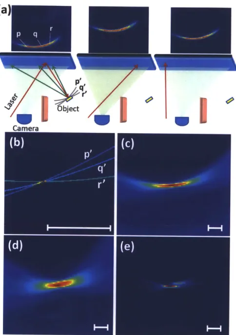
2-3 Reconstruction Algorithm An illustrative example of geometric

re-construction using streak images. (a) Data capture. The hidden object consists of a 2 cm x 2 cm square white patch. The captured streak images are displayed in the top row. (b) Contributing voxels in Carte-sian space. For recovery of hidden position the possible locations in Cartesian space that could have contributed to the streak image pixels p, q, r are ellipsoids in 3D. If there is a single world point contributing intensity to all 3 pixels, the corresponding ellipses intersect. The white bar corresponds to 2 centimetres.(c) Backprojection and heatmap. We use a back-projection algorithm that finds overlaid ellipses correspond-ing to all pixels.(d) Backprojection uscorrespond-ing all pixels in a set of 59 streak images. (e) Filtering. After filtering with a second derivative, the patch location and 2 centimeter lateral size are recovered. Joint work with Andreas Velten, Thomas Willwacher, Ashok Veeraraghavan, Moungi

G. Bawendi and Ramesh Raskar [41]. . . . . 41

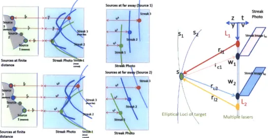
3-1 The top left figure shows streak images being generated by near field sources. On bottom left we see effect when this sources travel farther away, The rightmost figure depicts how we can analytically predict single sources using multiple sensor laser combinations. Notice how the accuracy is affected if lasers shift. . . . . 44

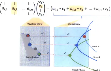
4-1 How each world voxel contributes to a streak inside data. The entire streak image is composed by linear sum of all the streaks. If there is no occlusion we can turn the forward model into a linear system and can generate a corresponding matrix representation. Vectorized world voxels (denoted by ci) on multiplication with linear transform matrix A yield streak image. The right hand is sum of streak images Aj corresponding to each voxel. . . . . 50

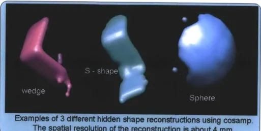
4-2 Our approach can handle steep angles, sharp corners, concave as well as convex features.Reconstruction of (a) Wedge (b) S shape and a (c) Sphere using 8 streak images and COSaMP matching pursuit algo-rithm. Referenced from joint work with Ashok Veeraraghvan in [41]. . 51

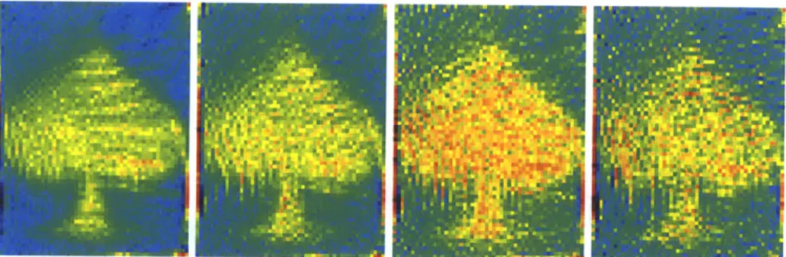
4-3 Reconstruction of a spade using plain linear inversion techniques. The matrix A was generated using methods described in section 4.1. We multiplied both sides with AT to make problem computationally feasi-ble. We used pseudo inverse implementation in MATLAB to find the solution . . . . 56

4-4 This figure shows how the reconstruction quality deteriorates by down sampling world voxels. (Left) Zero down-sampling (Middle) one third down-sampling (Right) One fifth down-sampling. . . . . 56

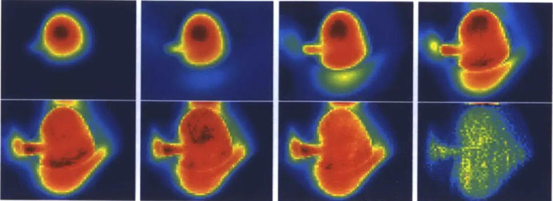
4-5 Above figure shows how spade evolves with every few iteration of

SPGL. Notice that the interior points get picked first. The last

im-age is result from 30 iterations. . . . . 57

4-6 Methods like SPGL requiring only single parameter have an optimal parameter value which results in correct reconstruction. The above figure shows the variation in error with variation in tau. This is in fact the pareto curve described in [6] between one norm of solution and two norm of residual. . . . . 57

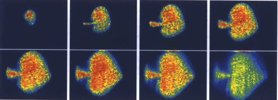
4-7 This figure shows how spade reconstruction changes with increasing tau. For lesser values of tau only interior points get selected and rest of shape remains unknown. As tau is increased the solution converges to a spade. . . . . 58

4-8 . Anaysis of reconstruction if random noise is added to parameters. The reconstruction is pretty robust to random salt and pepper noise in laser locations. . . . . 58

4-9 Random Salt and pepper noise in homography and its effect on recon-struction. _{. . . . 59} 4-10 Effect on reconstruction with systemic noise. . . . . 59

4-11 Variation in A with systemic noise. As we can see even small amount of homography error can change A significantly. . . . . 60

4-12 Effect on reconstruction with systemic noise in A. . . . . 60

4-13 (Above) Hidden MIT around the corner (Below) Reconstruction using

SPGL ... ... 61

5-1 The experimental setup. (B). The laser pulses strike the wall at a point

1

Veer-araghavan, Moungi G. Bawendi and Ramesh Raskar [41]. . . . .

65

5-2 Resolution in depth. Left: Distance estimation. Time here is measured

in mm of traveled distance at the speed of light 1 mmz0.3 ps. Middle: Error is less than 1 mm. Right: Plot of intensity as a small patch is moved perpendicular to the first surface. . . . . 66

5-3 Resolution in lateral dimension measured with a chirp pattern. (Left)

Setup with chirp pattern (occluder removed in this photo) (Middle) Raw streak photo from streak camera (Right) The blue curve shows reconstruction of the geometry and indicates that we can recover fea-tures with 0.5 cm in lateral dimensions in the given scenario. The curve shows the confidence in the backprojected values. . . . . 66

5-5 Reconstruction of a scene consisting of a big disk, a triangle and a square at different depth. (Left) Ground truth. (Middle) Reconstruc-tion, front view. (Right) ReconstrucReconstruc-tion, side view. Note that the disk is only partially reconstructed, and the square is rounded of, while the triangle is recovered very well. This illustrates the diminishing resolu-tion in direcresolu-tions parallel to the receiver plane towards the borders of the field of view. The blue planes indicate the ground truth. The gray ground planes and shadows have been added to help visualization. Referenced from joint work with Dr. Andreas Velten, Dr. Thomas Willwacher, Dr. Ashok Veeraraghavan, Dr. Moungi G. Bawendi and Dr. Ramesh Raskar [41]. . . . . 68

5-6 Challenges in imaging around the corner with a conventional, low tem-poral resolution laser and camera. (a) A setup with hidden mannequin but using a red continuous laser and a Canon 5D camera. (b) An image of the wall recorded with the Canon 5D camera with the room lights turned off and no hidden object present. (The recorded light is due to the reflections from walls behind the laser and camera.) (c) An im-age recorded with the hidden mannequin present. The increased light level on the wall is marginal, is low spatial frequency and shows no noticeable high frequency structure. (d) An image of the wall with the hidden mannequin moved away from the wall by 10 cm. The reduction in light level on the wall has no visible structure. (e) The difference between image in (b) and (c) using a false color map. (f) The difference between (b) and (d). (g) The difference between (c) and (d). (h) The plot of intensities along the centered horizontal scanline of each of the images (b=red, c=black, d=blue). . . . . 69

5-7 Limitations of heatmap after the backprojection algorithm. (Left) Propagation of a single point and its backpropagation for a flatland case. Reconstruction using backpropagation shows that one can re-cover a sharp peak, but it is surrounded by a low frequency residual. Y and Z sections are shown. The resolution in Y is lower than the resolution in Z. (Right) Cross Correlation of the streak images cor-responding to nearby voxels (3D case with 1D streak image). Notice that the Y-resolution is worse because the sensor is 1D along the x-axis. Results from joint work with Andreas Velten in [41]. . . . . 70

5-8 Reconstruction of a planar object in an unknown plane in 3D. (Left) The object. (Middle Left) 2D Projection of the filtered heatmap. (Mid-dle Right) A 3D visualization of the filtered heatmap. (Right) Recon-struction using sparsity based methods. The gray ground plane has been added to aid visualization. Referenced from joint work with Dr. Andreas Velten, Dr. Thomas Willwacher, Dr. Ashok Veeraraghavan, Dr. Moungi G. Bawendi and Dr. Ramesh Raskar [41]. . . . . 70

5-9 Reconstruction of a wooden man, painted white. Center - reconstruc-tion using simple back projecreconstruc-tion based methods. Right - reconstruc-tion using sparse reconstrucreconstruc-tion methods. Results from joint work with Andreas Velten in [41]. . . . . 70

5-10 Depiction of our reconstruction algorithm for a scene consisting of two

birds in different planes. (a) Photographs of the input models. (b) 9 out of 33 streak images used for reconstruction. (c) The raw (unfil-tered) backprojection. (d) The filtered backprojection, after taking a second derivative. (e,f) 3D renderings in Chimera. . . . . 71

5-11 The laser beam (red) is split to provide a syncronization signal for

the camera (dotted red) and an attenuated reference pulse (orange) to compensate for synchronization drifts and laser intensity fluctuations. The main laser beam is directed to a wall with a steering mirror and the returned third bounce is captured by the streak camera. An Occluder inserted at the indicated position does not significantly change the collected image. Referenced from joint work with Andreas Velten in [41]. 72

5-12 Smooth Object Reconstruction Reconstruction of two sinosoids

using SPGL1. (a) Photo of the object. The sinusoid is approximately

1.5 cm tall with total length of 5 cm. (b) Nine of the 60 raw streak

images. (c) Side View. Visualization of one cross sections from recon-struction. (d) 3D cross-sections. Chosen cross sections along depth (z) projected on the x-y plane reveals the hidden shape contour. (e) Top View. (f) Confidence map. A rendered point cloud of reconstruction values after soft threshold. . . . . 73 5-13 Complex Object Reconstruction in multiple poses. (a) Photo of

the object. The mannequin is approximately 20 cm tall and is placed about 25 cm from the diffuser wall. (b) Nine of the 60 raw streak images. (c) Heatmap. Visualization of the heatmap after backprojec-tion. The hidden shape is barely discernible. (d) Filtering. The second derivative of the heatmap along depth (z) projected on the x-y plane reveals the hidden shape contour. (e) Depth map. Color encoded depth shows the left leg and right arm closer in depth compared to the torso and other leg and arm. (f) Confidence map. A rendered point cloud of confidence values after soft threshold. (i) The stop-motion animation frames from multiple poses to demonstrate reproducibility. Shadows and the ground plane in images (f-i) have been added to aid visual-ization. Joint work with Andreas Velten, Thomas Willwacher, Ashok Veeraraghavan, Moungi G. Bawendi and Ramesh Raskar [41]. .... 74

5-14 Reconstruction of a hidden wood mannequin using sparse reconstruc-tion techniques . . . . 75

5-15 Demonstration of the depth and lateral resolution. (a) The hidden

object to be recovered are three letters, I, T, I at varying depths. The

"I" is 1.5 cm in wide and all letters are 8.2 cm high. (b) 9 of 60 images

collected by the streak camera. (c) Projection of the heatmap on the x-y plane created by the back projection algorithm. (d) Filtering after computing second derivative along depth (z). The color in these images represents the confidence of finding an object at the pixel position. (e) A rendering of the reconstructed 3D shape. Depth is color coded and semi-transparent planes are inserted to indicate the ground truth. The depth axis is scaled to aid visualization of the depth resolution. Referenced from joint work with Dr. Andreas Velten, Dr. Thomas Willwacher, Dr. Ashok Veeraraghavan, Dr. Moungi G. Bawendi and

Dr. Ramesh Raskar [41]. . . . . 76

5-16 Reconstruction of hidden ITI(MIT) using sparse reconstruction

tech-niques such as SPGL. Note that this result is from a technique entirely different from 5-15. (a) The hidden MIT. (b) Selected streak images. (c) Reconstructed volume with all sections merged into one image. (d) Volumetric slices of reconstructed hidden object. (e) The final result rendered in 3D (side view). Notice how accurately depth gets recov-ered. (f) Rendered MIT from front. . . . . 77

5-17 Results of a multi-pose stop motion animation dataset after filtered

backprojection and soft-thresholding. A hidden model of a man with a

ball is captured in various poses. The rendering shows the sequence of

reconstructions created by our filtered backprojection algorithm and demonstrates the ability to remove low-frequency artifacts of backpro-jection. The mislabeled voxels remain consistent across different poses indicating stability of our capture and inversion process. Shadows are introduced to aid visualization. Results from joint work with Andreas V elten in [41]. . . . . 78 5-18 Results from reconstruction of two cards using simple backprojection

techniques for real world data. (Left) The actual object. (Right) Re-constructed object. . . . . 78 5-19 Results from reconstruction of a wedge using simple backprojection

techniques, and carving in real world data. (Left) The actual object. (Right) Reconstructed object. . . . . 79 5-20 Results from reconstruction of a man using CoSAMP in simulation.

(Left) The actual object. (Right) Reconstructed object. . . . . 79 5-21 Results from reconstruction of a man using CoSAMP in simulation.

Chapter 1

Introduction

Current computer graphics and vision involve study of light coming from various points in visible in-line-of-sight world. Traditional imaging from cameras captures a fraction of light from scene, focuses it and integrates it on a sensor. A very high dimensional representation of scene involves parametrizing light intensity for each wavelength, in every direction coming from every visible point in the world. Concepts such as plenoptic function [4] can be used to describe response of an environment to current lighting conditions.

When we capture an image, light from non line of sight objects can also be imaged after reflections from visible objects. The effect of such light on our image is ignored because of its considerably lower intensity. The contribution of these photons is rendered insignificant by integration over much larger periods of time than time light took to move around in a scene. Of course this strategy is ignorant and wasteful of data. In this thesis we address the challenging problem of using these photons to resolve geometry of hidden objects.

1.1

Motivation

Very recently some interesting research has been done in the area we explore. In

[32, 31], Raskar and Davis proposed inverse analysis using a 5D time-light transport

of scene, camera and surrounding world, it is possible to image hidden aspects of scene

by switching lighting and cameras [35]. This approach can be used to get a faster 6D representation of scene as well. This approach requires a high resolution, highly

versatile light source like a projector focusing light at hidden object and therefore is not of much use in problem we describe. Highly sophisticated techniques such as LIDAR (LIght Detection and Ranging) [16] and two dimensional gated viewing [8] can be used to obtain low/high scale 3D representation of objects. Stealth technologies such as TADAR [7], infrared heat signatures can be used to look through diffused occluders such as walls. But all these technologies ignore the multiple reflections as noise and try to use filters to eliminate this information rather than use it for good. Can we exploit the time taken by photons to arrive to infer hidden 3D shapes ? In paper [17] an interesting technique is evolved which uses time of arrival of photons at high resolution to infer trivial information about scene like two dark lines separated

by white line. Our work builds on some of this work and develops a full conceptual

model of sensing photons after multiple reflections. Then we use this model to develop robust tools and infer shapes of 3D objects of varying complexity.

One may argue that TADAR is a good alternative to our strategies. In fact hidden imaging has always been approached as a problem involving sensing light transmitting through a diffuser which allows a few wavelengths which is a very strong assumption. But our approach provides a workaround to this obvious flaw, and makes no such assumption. Our final goal is to use photons which came after multiple reflections and determine the hidden objects. We believe that such an invention can revolutionize fields such as endoscopy, fast robot navigation, ultrafast reflectance capture and ultrafast geometry acquisition without worrying about occlusions.

1.2

Problem Description

We aim at exploring the relationship between hidden 3D structure of objects and the associated high dimensional light transport (in space and time). Our main emphasis will be on rigorously formulating the problem and developing methods to invert

tran-y

(

(x,y,)

L(x, y,

z,

0,

#)

9

Figure 1-1: Plenoptic function parametrizes world pixels by location, wavelength and orientation. (Source: Wikipedia)

sient light transport and recover hidden 3D shapes. In order to successfully invert the problem we will model the propagation of light in the scene, and its capture by cam-era. We will also focus at studying issues like existence and uniqueness of solution, and stability of solution algorithm.

We will exploit hardware such as streak cameras to image light with picoseconds level resolution in time. For determining accurate starting time of photons we will illuminate real world scenes using femtosecond duration pulses. Using this we can calculate distances travelled by photons with sub-millimeter level of accuracy.

While developing algorithms we aim at exploiting sparsity based methods to in-crease robustness and generate reconstruction for challenging inputs. We will develop models for various kinds of noises that might present in the process of capture, and observe how that might affect the results from reconstruction algorithm. We will validate the reconstruction algorithm using data collected in real world scenarios.

rr1 ₂ raft

UC0

Figure 1-2: Setup (Left). Forward model (Center) The laser illuminates the surface S

and each point

s

_{S generates an energy front. The spherical energy front contributes}

to a hyperbola in the space-time streak photo, IR. (Right) Spherical energy fronts

propagating from a point create a hyperbolic space-time curve in streak photo.

1.3

Related Work

Recent work in computer graphics and computer vision has shown surprising results

by inverting light transport. Our work is influenced by this pioneering work [34,

25, 35, 17, 21]. We also inspire from research in ultra fast imaging as discussed in

[24, 40, 45, 27, 31]. We will supplement the framework provided by these methods

by analysing and measuring the temporal evolution of light transport. Analysing the

energyfront propagation, we will exploit the added fine-scale time dimension to deal

with and recover the geometry of moderately complex hidden objects.

Comparison with Dual Photography and Transient Imaging: Light

trans-port acquisition, analysis and inversion is recently emerging to be a powerful tool to

extract intrinsic information about the scene even when the scene is hidden either

physically or because of global light transport effects. Sen et. al. exploited Helmholtz

reciprocity to recover view of a playing card visible to a light source but not to the

primal camera [35] at 66x87 pixel resolution. This does require a projector to be in

the line of sight. See figure 1-3.

Kirmani et. al. showed an intriguing idea of a time of flight camera to look

around corners. The results show how to read a mirror-based barcode beyond the

line of sight [17]. Given the challenging nature of the problem, they made strong

assumptions about the hidden points: they lie on a plane, the correspondence between time profiles of each point is recoverable and hidden points are not on a continuous surface (i.e. patches are discretized in position with gaps between the patches). This aids in marking contribution from each patch. This would be impractical in presence of real world continuous objects with unknown depth. Solving the problem in the absence of correspondences on three dimensional objects will be the key aspect of our work.

Range estimation using time of flight : Many techniques have been estab-lished for range estimation using time-of-flight measurements from active emission in a wide variety of electromagnetic and pressure-wave domains including radio fre-quency (RADAR), optical (LIDAR - see 1-5), and acoustic (SONAR - refer to 1-4)

[36, 15, 13]. However these techniques are limited by penetrability and the

assump-tion of single path and one-bounce reflecassump-tions. Multibounce RADAR has also been investigated, for example for motion detection [38]. Due to the longer wavelength of of RADAR, bounces are always specular and reconstruction is trivial. The resolution and capabilities are very limited.

Time of Flight and Scattering : In radio-location , geophysical surveys,

syn-thetic aperture radar and medical imaging, problems involve determining geometric information from scattered emission, reflection or transmission [23, 10, 28, 30, 42, 44]. For example, in radio-location, one can conveniently query the active emitter while in borehole tomography one can use one explosive source at a time to generate sig-nals which are picked up by receivers at the surface and in boreholes. The inversion is challenging because the emitters and receivers are sparse. Most problems also involve nonhomogeneous medium with varying refractive index. Kirchhoff integral techniques represent and solve the propagation with partial differential equations

[20, 18, 9, 37, 43]. The geometric solutions are relatively coarse and low resolution

and exploit transmission or one bounce reflection.

Apart from these the theory of inverse light transport [34] can be used to eliminate inter-reflections from real scenes. The frequency domain properties of direct and global components of scattered light can be exploited to recover image of objects

virtal camera

Dual Configuration

camfera

pixed

q

C"

I

scene

Figure 1-3: Dual Photography: Helmholtz Reciprocity. (Please refer to [35])

behind a shower curtain [25].

1.4

Contribution

We will explore the relationship between hidden 3D structure of objects and the

associated high dimensional light transport (space and time). We show that using

multi-bounce energyfront propagation based analysis one can recover hidden 3D

ge-ometry. We rigorously formulate the problem, elicit the relationships between

geom-etry and acquired light transport and also develop a practical and robust framework

for inversion. The specific technical contributions of the thesis are

Primal Configuration

p'

p

c'=Tp'

_q

cP

scene

AMEnHEEI

_n

=Tc

Figure 1-4: TADAR : millimeter wavelength imaging. Source [2]

" An algorithm for backpropagating the acquired space-time light transport to

overcomes the lack of correspondences and recover 3D shapes

" Exploiting sparsity based methods to reconstruct hidden 3D shapes

" An analysis of the invertibility and dependence on resolution of space-time

dimensions

" Several synthetic and physical experiments to validate the concepts

We will show that using multi-bounce energy front propagation based analysis

one can recover hidden 3D geometry. We analyze the problem of recovering a 3D

shape from its tertiary diffuse reflections. If there was only a single hidden point, the

reflected energy front directly encodes the position of that point in 3D. We rigorously

formulate the problem, elicit the relationships between geometry and acquired light

transport and also develop a practical and robust framework for inversion. We show

that it can be cast as a very peculiar type of tomographic reconstruction problem.

We call the associated imaging process elliptic tomography. The inverse problem,

i.e., the recovery of the unknown scene from the measurements, is challenging. We

provide a fast algorithm, which is essentially the analogue of the filtered

backprojec-z

- ROLL

ky

|

tion algorithm in traditional tomography. We perform several synthetic and physical experiments to validate the concepts.

Chapter

2

Theoretical Foundations

2.1

_{Modelling Propagation of a Light Pulse for}

Multiple Bounces

rcr.1 i,/c

Figure 2-1: Forward Model. (Left) The laser illuminates the surface S and each point

s

E S generates a energy front. The spherical energy front contributes to a hyperbola

in the space-time streak photo, IR. (Right) Spherical energy fronts propagating from

a point create a hyperbolic space-time curve in streak photo.

Consider a scene, as shown in Figure 2-1, which contains a hidden object (whose

surface we are interested in estimating) in front of a visible surface or 'first surface'

(this can be a wall or the floor). For simplicity we will assume that the visible

surface (hereafter called wall) is planar and diffuse, but we will relax this assumption

later. A laser beam(B) pointed towards the first visible surface (wall) to form a laser

spot L emits a very short (few picoseconds) light pulse. The light reflected by the

wall reaches the hidden surface, is reflected and returns back to the wall. A streak

camera pointed towards the wall records the time varying image on the wall at a

very high temporal resolution of around 2 picoseconds. Our goal is to understand the

relationship between the geometry of the hidden scene and the observed intensities

at each streak camera pixel and time bin.

(

This work was done in collaboration

with Dr. Andreas Velten, Dr. Thomas Willwacher, Dr. Ashok Veeraraghavan, Dr.

Moungi G. Bawendi and Dr. Ramesh Raskar [41].

)

For each location of the laser spot L, a 3D image (2 spatial and 1 temporal

dimension) is recorded. The laser spot is moved to multiple locations on the wall

(2D) to record 5D light transport data. The pulse return time at each location on

the wall depends upon several known parameters such as the location of the laser

spot and the unknown surface profile. So one can use the observed 5D light transport

data to infer the hidden surface shape. In order to understand the basic intuition,

consider the hidden scene to be a single point, as shown in Figure 2-1. The reflected

spherical wavefront propagating from that scene point reaches the different pixels on

the wall surface at different times creating a streak image which is a hyperbolic curve.

There is a one-one invertible mapping between the parameters of the hyperbola and

the 3D location of the hidden scene point.

When the hidden scene contains a surface instead of individual scene points, the

space-time hyperbolas corresponding to the different surface points are added together

to produce the captured streak images and so we need to demultiplex or deconvolve

these signals. In general, we could use a captured 5D light transport data but in our

experiments, we are restricted to a 1D streak camera. While the information from a

1D streak camera is sufficient for 3D reconstruction the spatial resolution in the axis

perpendicular to the sensor axis is heavily compromised.

It is convenient to move to the coordinate system of the wall. For this we apply

a space-time transform. We need to consider four optical path segments: beam B to

laser spot L on first surface, spot L to a hidden surface points s

E

S, s to points on

surfaces into a single 'wall' for compactness. With respect to the wall, the shape of the objects can be recovered as a 2D height field. By shining a short pulse duration laser and a recovering a full time profile of the returned signal, we capture a 5D light transport, 2D for camera pixels, 2D for laser projector positions and time. Thus, our inversion method needs to recover a 2D height map manifold from a 5D light transport data. As we show later, recovering this hidden 2D manifold with a 4D camera-projector light transport and without time-dimension is impractical due to ill-conditioning of the multiplexing matrix.

2.1.1

_{Space-Time Warping for Bounce Reduction}

Figure 2-2: A space time transform on a raw streak photo allows us to convert 4 segment problem into a sequence of 2 segment problems. The toy scene is a small lcmx 1cm patch creating a prominent (blurred) hyperbola in warped photo. Back-propagation creates low frequency residual but simple thresholding recovers the patch geometry.

For the looking around corner setup light path can be divided into 4 straight line segments with 3 bounces in between. The first segment involves collimated laser beam travelling from laser source to wall. In the second segment the laser spot on wall behaves as a point light source. The third segment(s) involve scattering from hidden object. For the fourth segment light travels from wall to camera which has wall in focus. The data received on camera Ic(p, t) has two degrees of freedom -space and time. Since first and fourth segments are focused, we can apply transforms to streak image to eliminate their effects. The effect of first segment can be removed

by shifting streak image in time which is constant for each location on wall. To

re-move effect of fourth segment we use the distances between wall pixels and camera sensors (II C - w _{1|). We assume that we know the geometry of R to calculate camera}

homography and correspondence between camera sensor and wall pixels. The fol-lowing mathematical formulation is concise representation of this concept. Here H is the projective transformation (homography) mapping coordinates on R to camera coordinates. The time shift IC - wIl by the distance from camera to screen varies

hyperbolically with the pixel coordinate w. Note that we don't require to adjust for cos(G) factor or 1/r2 fall off because camera sensor integrates for more wall pixels if they are farther away.

We can simplify the task of inference from four segment reflection paths to a sequence of two segment paths. First and fourth paths are directional and focused and do not involve scattering. The second segment can be treated as originating from unfocussed sensors while the third segment can be treated as being recorded by unfocused sensors. Our approach simplifies this three bounce problem to one bounce problem, by introducing corresponding space and time warps due to first and fourth paths. For the first path we calculate the time taken by laser to reach the wall and offset everything to include this. For the fourth path we compute the homography for streak camera imaging system and map the 1D image created on streak sensor to the wall in front. Then the pixels are offset in time to include the variation in time for light to reach the streak camera sensor. After discretization this situation is analogous to an unfocussed array of emitters and an unfocussed array of receivers. Unfortunately each of the emitters has a different phase depending on its position created due to its distance to laser spot and distance from the sensor. In addition the intensities are also impacted by aforementioned distances. Our goal is to recover from this multiplexed readings the location of each of transmitters.

2.1.2

Scattering of a pulse

Consider the impact of any scene point s E S on the recorded 5D light transport. The laser illuminates a point L on the visible surface of the wall and this in turn creates a virtual unfocused impulse light source. The light reflected from each scene point s is recorded by unfocused virtual sensors w E R. We model the impulse wave propagation from each scene point using the well-known Huygens-Fresnel principle.Phase changes

hyperbolically and intensity changes as r2 across the planar section for the wavefront. This hyperbolic streak, or 'streak' for short is captured by a streak camera.

Generating Streak Photos

Let's analyze the scattering of light in second and third segments. For simplicity we model the hidden object as a collection of unfocussed emitters sending impulses I, (s, T) at T _{times. We model the receiver as an array of unfocussed receivers which}

capture photons at picosecond resolution. We can achieve this configuration experi-mentally by using a picosecond resolution streak camera focused on wall pixels. To simplify further we can assume accurately that speed of light is constant and ex-press everything in distance units. The following mathematical equation represents the data recorded by streak camera after making the mentioned assumptions. Note that speed of light is set c=1 for simplicity. We also ignore the local changes in nor-mals for sender surface and receiver surface. (Algorithm programming with Thomas Willwacher and data collection with Andreas Velten, results in paper [41].)

IR(W, t) -

j j

where w E R, s E S, t,T E R and rc =

11w

section and applying transforms from calculated homography we can further simplify the equation and remove the 6 required to adjust for receiver camera distances. The following equation provides the mathematical summary of this analysis. Note that overall these equations we assume that receiver and senders are perfectly lambertian and ignore the local superficial variation in Normal vectors. Equation (2.1) hence becomes

IR 0 1 1 2 126(t

-r, -ri)d2s(2)

2.1.3

Hyperbolic Contribution

Hyperbolic Contribution

Lets analyze the relationship between time when a sender emits a pulse to time and location of a receiver. For a fixed sender the response function is a hyperboloid in space and time given by following mathematical equation. The parameters of the hyperboloid depend on location of sender, a lateral displacement leads to shifts, while a displacement in depth corresponds to flattening. Change in sender time equates to a constant time shift for responses to any of receivers.

t-r = rc = V(zX -U)2 + (y - v)2+z(x,y)2 (2.3)

where u, v are the two coordinates of w in the receiver plane. Careful observation shows that this equation is an ellipsoid in sender location if we fix the laser and receiver location. Ellipse parameters depend on time when a receiver receives a impulse. The laser and receiver lie on the two focii of this ellipse. The eccentricity depends on the time when impulse is received.

2.2

_{Forward model: Elliptical Tomographic}

Pro-jection

In this section we rephrase the above approximation to the forward light transport using notions from tomography. In an idealized case, the inverse problem of recovering the hidden shape can be solved explicitly. We use this explicit solution to inspire our algorithm for real world scenarios. This work was done in collaboration with Dr. Andreas Velten, Dr. Thomas Willwacher, Dr. Ashok Veeraraghavan, Dr. Moungi G. Bawendi and Dr. Ramesh Raskar [41].

2.2.1

Elliptical tomography problem description

Our problem has similarities to tomographic projection. Let us rewrite equation (2.2) in the following form

IR(W,t, L) - I 2 6(t - re -ri)d2S = 2 6(t- r - ri)Is(x)daX

is 7rrwrri s 7rc rri

S 221 6(t - r - ri)W(x)d x

where the unknown world volume W(x) = I6s(x) is a delta function with support on the surface S to be reconstructed. Apart from the 1/r 2

factors, which typically vary slowly over the region of interest, we hence see that individual streak image pixels measure elliptical projections of the world volume W(x). Due to its similarity with traditional tomography, we call this problem elliptical tomography. Note however that there are also key differences to traditional tomography: (i) The recorded projections live in a higher dimensional (5D) space than the world (3D). (ii) The projections are along (2D) ellipsoids instead of (ID) lines. This makes the analysis much more complicated.

2.2.2

Challenges and missing cones

It is instructive to consider the above tomography problem in the limit when the object is small compared to the distance to the diffuser wall. In this case the elliptic tomography problem reduces to a planar tomography problem, see Figure 3-1. Each pair of a camera point and a laser position on the diffuser wall (approximately) measures intersections of the target object with planes whose normals agree with the normals to the ellipsoids. By the standard Fourier slice theorem, each line of each streak image will hence measure one line of the Fourier transform of the object, in the direction of the normal. Unfortunately, in our situation these normals cover a limited region of the unit sphere. Hence without additional priors it is not possible to reconstruct the Fourier transform of the target object in the missing directions. This is the missing cones problem well known from traditional tomography. Experimentally

we get a very good resolution in the depth (orthogonal to the wall) direction, while transverse (parallel to the wall) high frequency features tend to get lost.

Figure 2-3: Reconstruction Algorithm An illustrative example of geometric

re-construction using streak images. (a) Data capture. The hidden object consists of a 2

cm x 2 cm square white patch. The captured streak images are displayed in the top

row. (b) Contributing voxels in Cartesian space. For recovery of hidden position the

possible locations in Cartesian space that could have contributed to the streak image

pixels p, q, r are ellipsoids in 3D. If there is a single world point contributing intensity

to all 3 pixels, the corresponding ellipses intersect. The white bar corresponds to 2

centimetres. (c) Backprojection and heatmap. We use a back-projection algorithm that

finds overlaid ellipses corresponding to all pixels.(d) Backprojection using all pixels

in a set of 59 streak images. (e) Filtering. After filtering with a second derivative, the

patch location and 2 centimeter lateral size are recovered. Joint work with Andreas

Velten, Thomas Willwacher, Ashok Veeraraghavan, Moungi G. Bawendi and Ramesh

Chapter 3

Inversion Analysis

3.1

_{Inverse Algorithm: Filtered Back Projection}

In this section we give a detailed description of our reconstruction algorithm. (Al-gorithm programming with Thomas Willwacher, Andreas Velten and data collection with Andreas Velten, in collaboration with Dr. Ashok Veeraraghavan, Dr. Moungi

G. Bawendi and Dr. Ramesh Raskar [41].)

3.1.1

Overview of the algorithm

The imaging and reconstruction process consists of 3 phases:

" Phase 1: Data Acquisition. We direct the laser to 60 different positions on

the diffuser wall and capture the corresponding streak images. For each of the

60 positions more than one images are taken and overlaid to reduce noise. * Phase 2: Data Preprocessing. The streak images are loaded, intensity

corrected and shifted to adjust for spatiotemporal jitter.

" Phase 3: 3D Reconstruction. The clean streak images are used to

recon-struct the unknown shape using our backprojection-type algorithm.

The first of the three phases has been described in chapter 1 and 2. Let us focus on Phases 2 and 3.

Streak Photo 1 W2 Ll22 Sources at fink@t dtasce

Figure 3-1: The top left figure shows streak images being generated by near field

sources. On bottom left we see effect when this sources travel farther away, The

rightmost figure depicts how we can analytically predict single sources using multiple

sensor laser combinations. Notice how the accuracy is affected if lasers shift.

3.1.2

Phase 2: Data Preprocessing

1. Timing correction. To correct for drift in camera timing synchronization

(jitter) both in space and time we direct part of the laser directly to the diffuser

wall. This produces a sharp "calibration spot" in each streak image. The

calibration spot is detected in each image, and the image is subsequently shifted

in order to align the reference spot at the same pixel location in all streak

images. The severity of the jitter is monitored in order to detect outliers or

broken datasets. (Data collection with Andreas Velten, results in paper [41].)

2. Intensity correction. To remove a common bias in the streak images we

subtract a reference (background) image taken without the target object being

present in the setup.

3. Gain correction. We correct for non-uniform gain of the streak camera's CCD

sensor by dividing by a white light image taken beforehand.

3.1.3

Phase 3: 3D Reconstruction

1. Voxel Grid Setup. We estimate an oriented bounding box for the working

volume to set up a voxel grid (see below).

2. Downsampling (optional). In order to improve speed the data may be

down-sampled by discarding a fraction of the cameras pixels for each streak image and/or entire streak images. Experiments showed that every second camera pixel may be discarded without losing much reconstruction accuracy. When discarding entire streak images, is is important that the laser positions on the diffuser wall corresponding to the remaining images still cover a large area.

3. Backprojection. For each voxel in the working volume and for each streak

image, we compute the streak image pixels that the voxel under consideration might have contributed. Concretely, the voxel at location v can contributed to a pixel corresponding to a point w on the wall at time t if

ct = |v - L| +Iv - w|+|w -- C|.

Here C is the camera's center of projection and L is the laser position as above. Let us call the streak image pixels satisfying this condition the contributing

pixels. We compute a function on voxel space, the heatmap H. For the voxel

v

under consideration we assign the value

H(v) =

Z(|v - w||v -

P

Here the sum is over all contributing pixels p, and I, is the intensity measured at that pixel. The prefactor corrects for the distance attenuation, with a being some constant. We use a = 1.

4. Filtering. The heatmap H now is a function on our 3 dimensional voxel grid. We assume that the axis of that grid are ordered such that the third axis faces away from the diffuser wall. We compute the

filtered

derivative of the heatmap along that third axis of the voxel grid.

Hf

The filtered heatmap measures the confidence we have that at a specific voxel location there is a surface patch of the hidden object.

5. Thresholding. We compute a sliding window maximum M₁,c of the filtered

heatmap Hf. Typically we use a 20x20x20 voxel window. Our estimate of the

3D shape to be reconstructed consists of those voxels that satisfy the condition

H

> A

+

where Mglob = _{max(Hg) is the global maximum of the filtered heatmap and} Aloc, Agio are constants. Typically we use Ao = 0.45, Ag91o = 0.15

6. Compressive Reconstruction

We use techniques like SPGL1, and CoSAMP as an alternative to back projec-tion and filtering. We rely on the fact that the 3D voxel grid is sparsely filled, containing surfaces which can occupy only one voxel in depth.

7. Rendering. The result of thresholding step is a 3D point cloud. We use the

Chimera rendering software to visualize this point cloud.

In order to set up the voxel grid in the first step we run a low resolution version of the above algorithm with a conservative initial estimate of the region of interest. In particular, we greatly down sample the input data. By this we obtain a low resolution point cloud which is a coarse approximation to the object to be reconstructed. We compute the center of mass and principal axis of this point cloud. The voxel grid is then fit so as to align with these axis.

3.2

Inversion using parameter estimation

Another good approach that we could use for reconstruction involves modeling cap-tured data as collection of hyperbolic streaks with unknown parameters. We can formulate this problem as optimization problem where we are trying to fit a conic section (hyperboloid) to a streak, minimizing total number of hyperbolas fitted. As discussed in next chapter this can be achieved by imposing a sparsity constraint on re-constructed world. In a very simple model each active pixel corresponds to a unique hyperboloid and we are trying to minimize number of active pixels while reducing residual errors. We can describe the residual error by following equation:

J(X, t) - S, * 6(x2/a - t2/bi - 1)112 (3.1)

(x,t)eStreakImages i6ActivePixels

Here I(x, t) is the recorded streak image, ai and bi are paramters for streak cor-responding to active pixel and Si is corcor-responding intensity. We can then include the sum of all active voxels or number of active voxels as a regularization parameter to complete the formulation. The main issue with this formulation is that actual streaks have a lot of blur and noise, and it can lead to a lot of computation overhead because of large parameters. Also because of systematic noise we cannot be sure that hyperbolas will overlap exactly. To overcome this issue, instead of fitting the pixels exactly we can minimize their from distance from the hyperbolas.

Their are two interesting observations to make about this technique. For scenes with isolated patches, we could reduce our search space to a few parameters. For scenes with continuous random surfaces, this search space grows infinite and needs to be discretized. A robust way to estimate the active voxels can be to use hough trans-form. Very simply, we can overlay the streak image due to each voxel and integrate to get a likelihood estimate for that voxel being active. We can use appropriate threshold to decide which voxels to choose. This technique is exactly same as backprojection technique we discussed earlier.

3.2.1

A remark about the filtering step

To motivate our choice of filter by taking the second derivative, let us consider again the planar ("far field") approximation to the elliptical tomography problem as dis-cussed in section 2.2.2. In this setting, at least for full and uniform coverage of the sphere with plane directions, the theoretically correct filtering in the filtered back-projection algorithm is a |k12

filter in Fourier space. In image space, this amounts to taking a second derivative along each scanline. This motivates our choice of filter above. We tested both filtering by the second derivative in image and world space and found that taking the derivative approximately along the target surfaces normal yielded the best results.

Chapter 4

Sparsity Based Reconstruction

In this chapter we show how we can use SPGL1 and other compressive sensing tech-niques to reconstruct hidden volumes. Because we aim at reconstructing hidden object's 2D manifold, we can consider the solution as a sparse set of points inside the voxelized world volume. This approach has many advantages over the simple back-projection based techniques. This approach actually inverts the system in front of us instead of using a voting technique like backprojection or carving. This approach will also minimize noise by choosing accurate parameters. Further as results show, this technique can yield much better results than ad-hoc approaches like backprojection.

4.1

Linearizing The system

Consider a isolated voxel in world, and focus on response it produces in streak images. The response changes orientation in time and space based on the laser location and wall pixels being observed. The response observed at each pixel on wall is a linear time invariant sum of time signals sent by all active world voxels. In essence to get any streak image we can add streak images from all world voxels provided that occlusion doesn't occur. We can construct a large matrix to represent this system, we denote the corresponding linear transform by matrix A. Each column of this matrix represents the streak image from corresponding world voxel. Each row in corresponding linear transform matrix A identifies a unique pixel,laser-location pair. This matrix can be

c,

ail,

a

(ai,

W O .bId Streak Image

StrStreak 3

Streak 2

Streak Photo k 1

Figure 4-1: How each world voxel contributes to a streak inside data. The entire

streak image is composed by linear sum of all the streaks. If there is no occlusion we

can turn the forward model into a linear system and can generate a corresponding

matrix representation. Vectorized world voxels (denoted by

c

)

on multiplication with

linear transform matrix A yield streak image. The right hand is sum of streak images

Aj corresponding to each voxel.

used to quickly draw streak images and backproject. The matrix comes to roughly 1

billion entries, and can easily takes Gigabytes of space. The matrix is practical only

if the voxelized world is small in size or we are willing to sacrifice resolution. (please

refer to 4-1)

Since number of wall pixels and laser locations is considerably more than world

voxels, size of corresponding linear transform matrix A can be reduce by sub sampling

world voxels and selecting only a few lasers. This too leads to poorer reconstruction

(4-4) but the results are a lot better than slashing down resolution.

Once we have a matrix to represent our system, we can try to invert the system

by solving linear system Ax

_{B. However using least square or inverting the system}

is a naive approach and can be computationally heavy. A easy solution is to reduce

number of columns of the linear system by multiplying by a well suited matrix M on

both sides (MAX

Mb). In our problems we used

_{to conserve rank and create}