Generalizing Ripley's K function to inhomogeneous populations

HAL Id: halshs-00372631

https://halshs.archives-ouvertes.fr/halshs-00372631

Preprint submitted on 1 Apr 2009

HAL is a multi-disciplinary open access archive for the deposit and dissemination of sci-entific research documents, whether they are pub-lished or not. The documents may come from teaching and research institutions in France or

L’archive ouverte pluridisciplinaire HAL, est destinée au dépôt et à la diffusion de documents scientifiques de niveau recherche, publiés ou non, émanant des établissements d’enseignement et de recherche français ou étrangers, des laboratoires

Generalizing Ripley’s K function to inhomogeneous

populations

Eric Marcon, Florence Puech

To cite this version:

Eric Marcon, Florence Puech. Generalizing Ripley’s K function to inhomogeneous populations. 2009. �halshs-00372631�

G

ENERALIZING

R

IPLEY

'

S

K

F

UNCTION TO

I

NHOMOGENEOUS

P

OPULATIONS1

E

RIC

M

ARCON2 AND

F

LORENCE

P

UECH3

1

We wish to thank Gabriel Lang for his helpful comments.

2 Corresponding author, AgroParisTech ENGREF, UMR EcoFoG, BP 316, 97310 Kourou, French Guyana. E-Mail: [email protected]

3 LET (Université de Lyon, CNRS, ENTPE), Institut des Sciences de l’Homme, 14 av. Berthelot, 69363 Lyon Cedex 07, France. E-Mail: [email protected]

Abstract:

In spatial statistics, Ripley’s K function (Ripley (1977)) is a classical tool to analyse spatial point patterns. Yet, it faces two major limits: it is only pertinent for homogeneous point processes and it does not allow the weighting of points.

We generalize it to get a new function, M, which oversteps these limits and detects spatial structures of inhomogeneous populations of weighted points.

1 Introduction

The basic analysis of a point set relies on its first-order property, that is to say the average values of chosen variables. An example is given by foresters who classically describe a forest plot with the histogram of tree diameters. This is enough for forestry management, but some scientific fields (like ecology) study the way species interact with each others, tackles new questions: how do these trees occupy space? Do trees of the same species aggregate or repulse each other?

New tools have progressively been developed to rigorously answer these more complicated questions. A major milestone was established by Clark and Evans (1954). The general method was given: measure a pertinent variable (the distance from every object to its nearest neighbour) and compare its value to the one that would have been given by randomness. Next, a fundamental step was made by Ripley (1976) who wrote the full theory of the second-order properties of point processes, giving the framework for better tools, taking into account all neighbours rather than only the nearest. Ripley (1977) then introduced the K function to analyse point-set structures. This function has been widely used for 25 years and became a standard measure presented in spatial statistic handbooks (Ripley (1981), Diggle (1983), Upton and Fingleton (1985), Cressie (1993)). However, Ripley’s K function faces two important limits: it supposes homogeneous space, and considers all points as equivalent (i.e. points’ characteristics do not matter). Therefore, this tool seems to be inappropriate to analyse obviously non-stationary point sets or objects whose size matters, like the study of the spatial structure of manufacturing plants (Marcon and Puech (2003a)). A first solution was given by Cuzick and Edwards (1990) who developed a non-parametric test able to detect clustering in a non-homogeneous point set, followed by Diggle and Chetwynd (1991) who introduced the D function, defined as the difference between the K function for studied points (called cases) and the K function for the others (called controls). This is not completely satisfactory yet because, since both K functions are computed separately, all the data contained in the relative position of cases and control is lost.4 Baddeley et al. (2000) generalize K to inhomogeneous point processes. They give a clean theoretical framework but practical applications are difficult, as we will se here. Therefore, the purpose of this study is to give a mathematical framework of a new measure, namely the M function, which oversteps these limits and actually detects spatial structures of inhomogeneous populations of weighted points.5

The paper is organised as follows. The next two parts recall the important features of point processes and that of Ripley’s K function. Part 4 constitutes a discussion on some features of Ripley’s K function to open the way (part 5) for its generalisation to inhomogeneous space and weighted points, introducing the M function. A comparison with Baddeley’s Kinhom is

developed.

2 Point processes

A point process is the equivalent of a random variable whose result is a point, defined by its coordinates (x, y) in a pre-defined area that we will call the domain, known and delimited.

4

Point processes are used as mathematical tools to characterize and eventually model events whose spatial repartition is known, such as trees in a forest.

An interesting way to describe an unknown-law process is through its first and second-order properties.

2.1 First-order property Definition

Consider an area A supplying a realization of a point process. N is the actual number of points inside A. Each point is defined by its coordinates (x, y). We denote N(S) the number of points inside a given sub-area S.

The process first-order property is its density, denoted λ(x, y). Its definition is:

dS dS N E y x dS )] ( [ lim ) , ( 0 → = λ (1)

where dS is the elementary area around (x, y).

If λ(x, y) is a constant, we will say the point process is homogeneous or stationary, and the

density will just be denoted λ.

Probability to find a point in an elementary area

We will only consider ordered point processes (Diggle (1983), p.47), i.e. the magnitude of the probability to find several points in an elementary area dS is smaller than dS. In other words, we will be allowed to write that the probability to find several points in dS is almost equal to the probability to find one only.

This assumption is not restrictive. To get convinced, consider a process providing independent points. The probability to find two points in dS is (PdS)2. According to the

first-order property, it equals [λ(x,y)dS]2. Since dS is small, (dS)2 is negligible compared to dS. This property establishes the linkage between probability and density. The existence of a point in dS is the result of a Bernoulli proof of parameter PdS. The number of points in dS thus

follows a Bernoulli law and its expectation is PdS. According to equation (1), this expectation

is λ(x, y).

The probability to find at least one point in the elementary area dS around the point located at

(x, y) is consequently:

dS y x

P_dS =λ( , ) (2)

This relation is verified as long as dS is small enough for the probability to find two points remains negligible.

2.2 Second-order property

Definition

2 1 2 1 0 , 2 2 1 1 2 )] ( ) ( [ lim )) , ( ), , (( 2 1 dS dS dS N dS N E y x y x dS dS → = λ (3)

Probability to find two points in two elementary areas

The joint probability to find at least one point in each elementary area around (x1,y1) and (x2,y2) is denoted PdS1,dS2. Once again, the probability to find more than one point in an area is

negligible. The event “find both a point in dS1 and in dS2” realizes a Bernoulli proof with

parameter PdS1,dS2, so: )) , ( ), , (( _{1 1 2 2} 2 2 1 , 2 1 dS dS x y x y P_{dS dS} = λ (4)

Introducing the first-order property:

) , ( ) , ( )) , ( ), , (( 2 2 1 1 2 2 1 1 2 , 2 1 2 1 y x y x y x y x P P P_{dS dS dS dS} λ λ λ = (5) The expression ) , ( ) , ( )) , ( ), , (( 2 2 1 1 2 2 1 1 2 y x y x y x y x λ λ λ

, ratio of the second-order to the first-order property, is called radial distribution function (Diggle (1983)), or point-pair correlation function (Cressie (1993)). We follow Ripley (1977) and the following literature, denoting it g((x1,y1),(x2,y2)).

Common usage (for instance Ripley (1977), Stoyan et al. (1987)) imposed g rather than λ2 as the measure of the second-order property. We will follow it:

2 1 2 1, 2 2 1 1, ),( , )) (( dS dS dS dS P P P y x y x g = (6)

If the process is isotropic, g(•) only depends on the distance between points and it will be

denoted g(r). In the case of an independent point distribution, the joint probability is equal to the product of the individual ones, thus g(•)=1. An independent point process is isotropic. 2.3 The homogeneous Poisson process particular case

Complete Spatial Randomness (CSR) is defined by homogeneity and independency.

The homogeneous Poisson point process gives completely random points. Inversely, a completely random point process is a homogeneous Poisson process (proof in Diggle (1983), p.50-51).

First-order property

A realization of a homogeneous Poisson process with parameter λA on the area A is a

completely random point set of density λ. The number of points follows a Poisson law with parameter λA, that is to say that:

k! A e k P(N k A ( ) )= −λ λ = (7)

This property remains true for any area S chosen within A. The number of points inside it follows a Poisson law: its expectation is λS, its variance is λS (a completely random

distribution is not regular). A non-homogeneous Poisson point process is defined similarly, with λ depending on the location. In what follows, we will only consider homogeneous Poisson processes (except if it is explicitly mentioned).

Second-order property

Since point are distributed independently from each other, g(•)=1.

The Poisson process will be used as the reference for complete spatial randomness (CSR), to compare the actual point distributions with.6

3 Ripley’s K function

The K function, defined by Ripley (1976); Ripley (1977) is a good indicator for spatial structures (Besag (1977), Diggle (1983), Cressie (1993)). Here, we will only consider homogeneous and isotropic point processes.

3.1 Introduction: probability to find a neighbour at a given distance

We call a point i’s neighbours all the points located at a distance lower than or equal to a given value r (basically, it represents the count of neighbours in a circle of radius r centered on the point i). The number of neighbours’ expectation is denoted v(r). Its estimator, the observed number of neighbours, is denoted V(r). Ripley (1977) showed that:

∫

= = r g d r v 0 2 ) ( ) ( ρ ρ πρ ρ λ (8)

3.2 Definition of the K function

Ripley (1977) defined the K function as:

∫

= = r d g r K 0 2 ) ( ) ( ρ ρ πρ ρ (9)

If points are distributed independently from each other, g(ρ)=1 for all values of ρ, so

K(r)=πr2. This value is used as a benchmark:

• K(r)> πr2 indicates that the average value of g(ρ) is greater than 1. The probability to

find a neighbour at the distance ρ is then greater than the probability to find a point in the same area anywhere in the domain: points are aggregated.

6

• Inversely, K(r)< πr2 indicates that the average neighbour density is smaller than the average point density on the studied domain. Points are dispersed.

K(r) is estimated by the ratio of the average number of neighbours on the density, estimated

itself by the total number of points divided by the domain area (

A N = ∧ λ ): A N r V r v r K( ) = (_∧ ) = ( ) ∧ ∧ λ (10)

The average number of neighbours can be expressed more explicitly by defining the indicator

c(i,j,r)=1 if the distance between points i and j is at most r, 0 otherwise:

∑ ∑

= = ≠ ∧ ∧ = N i N j i j c i j r N r K 1 1, (, , ) 1 ) ( λ (11)

3.3 Correction of the edge effects

Points located close to the domain borders are problematic because a part of the circle inside which points are supposed to be counted is outside the domain. Ignoring this edge effect results in underestimating K.

Ripley’s correction

Ripley (1977) proposed to correct the indicator c(i,j,r) introduced in equation (11).

We denote Ljr the portion of the circle of radius r centred on the point i located inside the

domain. If a part of the crown of width dr inside which a neighbour is counted is outside the domain, the neighbour is given a weight equal to the inverted ratio between the inside part of crown (Ljrdr) and the whole crown (2πrdr). The idea is that the outside part of the crown

could have contained the same neighbour density than the inside part. The correction is:

∑ ∑

= = ≠ ∧ ∧ = N i N j i j ir r j i c L r N r K 1 1, ( , , ) 2 1 ) ( π λ (12) Besag’s correction

Besag (1977), in his discussion of Ripley’s paper, underlined that this correction gave an excessive weight to the farthest neighbours. The greater the radius r, the smaller Ljr, and the

bigger the correction. He proposed an alternative: correct the edge effect not for each neighbour, but for all of them the same way.

We denote Air the part of the area of the circle of radius r centred on the point i located inside

the domain. We count the number of neighbours inside the circle and we correct it by the ratio between the circle’s area and its inside part. We suppose that the outside part of the circle would have contained the same neighbour density than the inside part. Finally:

∑

=

∑

= ≠ ∧ ∧ = N i N j i j ir r j i c A r N r K _{1 1,} 2 ) , , ( 1 ) ( π λ (13)

Even though these edge-effect corrections methods are used alternatively, Ripley’s is still widely applied in the literature (see for instance Haase (1995)).

Ward and Ferrandino’s correction

Ward and Ferrandino (1999) introduced a global correction, arguing that local correction methods depend on the number and position of points close to the borders, thus introducing more variability in K’s estimator.

They proposed to evaluate the expectation of the number of points concerned with edge-effect correction for a given radius (this is not a problem since the point process is supposed to be homogeneous), compute the correction for them (by the Besag’s method) and finally calculate the global underestimation of the number of point pairs which only depends on the domain’s geometry. They denoted KA (A for analytical) their estimator of K defined by:

∑ ∑

= = ≠ ∧ ∧ − = N i N j i j A c i j r r C N r K 1 1, ( , , ) ) ( ) 1 ( 1 ) ( λ (14)

C(r) is the global correction factor. For a rectangular (L by W) domain, they found (as long as r < W/2): ⎟⎟ ⎠ ⎞ ⎜⎜ ⎝ ⎛ ⎟ ⎠ ⎞ ⎜ ⎝ ⎛ ₋ + ⎟ ⎠ ⎞ ⎜ ⎝ ⎛ + − = WL r W r L r ) r ( C 2 1 3 11 3 4 1 π π (15)

Note that they did not justify the replacement of N by N-1 in the denominator of the estimator. We will explain the importance of this change, further.

Additionally, the authors calculated the variance of their estimator and its confidence interval. They claimed that their estimator both reduces K’s estimation bias and increases its efficiency and they justified this by several examples.

Other correction methods

The other correction methods are much more anecdotic. The most simple of all consists in using a buffer zone around the domain. The buffer is used to count neighbours but reference points (the points i) are never taken inside it. The buffer width is equal to the largest value of r so no edge effect ever appears. Since the buffer zone contains as much data as the domain, considering that most of the work is collecting data, the temptation is great to include the buffer into the domain: this method is very rarely used (examples can be found in Szwagrzyk and Czerwczak (1993), Kuuluvainen and Rouvinen (2000), fig.1a, p.803). The toroidal correction consists in treating the domain as a torus, that is to wrap it so that its opposite borders are in contact, supposing of course that its shape allows it. A good illustration is given by Haase (1995), fig.3, p.578. This solution is intuitively little satisfactory because it considers that the opposite points as very close. It was used by Peterson and Squiers (1995) and Kuuluvainen and Rouvinen (2000).

Empirical issues due to the edge-effect correction may be considerable. Getis and Franklin (1987) give formulas for a rectangular domain, Diggle (1983), p.72, for a rectangle and a

circle. Haase (1995) reviews and compares correction methods: Ripley’s, the buffer zone, and the torus. He notices and corrects an error in Diggle’s list of cases needing a correction, leading to a serious underestimation of K and a little error leading to a slight overestimation in Getis and Franklin’s formulas. Goreaud and Pélissier (1999) developed algorithms to study more complex domains, implemented in ADE software (Thioulouse et al. (1997)). Treating complex geographical limits such as a country’s boundaries is possible, but was never applied in the literature: the domain is always a polygon (Sweeney and Feser (1998), fig.1, p.52, Rowlingson and Diggle (1993), fig.5, p.634), or, more rarely, a circle (Pancer-Koteja et al. (1998), fig.1-3, p.757).

3.4 Besag’s L function

Ripley’s function is not very convenient to use. Comparing a computed value to its benchmark, πr2, implies more computing and the hyperbolic chart is not very expressive. Besag (1977) proposed to normalize the function to obtain a benchmark of zero:

r r K r L = − π ) ( ) ( (16) 3.5 Significance

The estimated values of K and L are compared to benchmarks given by a homogeneous Poisson process. To test whether a value of L(r)

∧

is significantly different from 0, the most common way is using the Monte Carlo technique (Diggle (1983)):

• A great number of random data sets is generated. Each of them is consistent with the null hypothesis tested.

• A confidence threshold α is chosen. • For each value of r, L(r)

∧

values are sorted in increasing order. The nth value is denoted Ln(r)

∧

.

• Extreme values are eliminated: the null hypothesis confidence interval limits are ) ( ) 2 ( r LN α ∧ and LN(1−α 2)(r) ∧

. For N=1000 and α=5%, we retain the 26th and the 974th

values. • L(r)

∧

is considered significantly different from 0 if its value is outside the interval )] ( ); ( [LN(α 2) r LN(1−α 2) r ∧ ∧ .

Attempts to directly calculate the confidence interval can be found in the literature. Ripley (1979) respectively proposed 1 42 , 1 − ± N A and 1 68 , 1 − ± N A

as approximations of the interval limits at 5% and 1% thresholds. These values were obtained from simulations. Due to the lack of theoretical background, these values are very little used (for example by Szwagrzyk and Czerwczak (1993)).

4 Discussions on Ripley’s K function

4.1 Global confidence intervals

4.2 Edge-effect corrections

Correcting the edge effects by Ripley’s method, equation (12), is impossible if a single value of Ljr equals 0, that is, as soon as r is big enough for a circle around a point to be completely

outside the domain. If the domain is a rectangle, K’s computation is thus limited to half of its length. Diggle (1983), p.72, gave correction formulas applicable up to half of the width. Goreaud and Pélissier (1999) improved the edge-effect correction to allow computing K up to half of the rectangle’s length.

We will rather use Besag’s method, equation (13), which is not limited. Detailing the density estimator, we get the expression of K, corrected from the edge effect:

∑

=

∑

= ≠ ∧ = N i N j i j ir r j i c A r N A r K _{1 1,} 2 2 ( , , ) ) ( π (17) 4.3 Correction of K’s bias Let us calculate K(r) ∧

according to equation (17) for a great value of r, such as the part of domain area included in each circle is the domain itself: Air=A for all points i. Thus, every

point’s distance to any other is smaller than r: c(i,j,r)=1. We can calculate K:

N N r A r N A r K( ) _iN₁ N_{j 1,i j}1 2 1 2 2 − = =

∑

₌

∑

_{= ≠} ∧ π π (18)

This result is problematic: the point set structure is homogeneous by assumption, so K should tend to πr2. This issue is rarely mentioned in the literature because Ripley’s edge-effect correction method limits r to a fraction of the domain’s size. Getis (1984) remarks that the number of point pairs is N(N-1), so an unbiased estimator of the squared density is N(N-1)/A². Getis and Franklin (1987) use it without further explanations. Diggle and Chetwynd (1991) indirectly evoked it when they gave a different formulation for K “to get an unbiased estimator of K”, without explaining the reason. Sweeney and Feser (1998) used the methods from Diggle and Chetwynd (1991) including their unbiased estimator. Moeur (1993) wrote that the estimator is biased, but only slightly, and used the same formula. Finally, Jones et al. (1996) used an unbiased formulation consistent with equation (19), below, justifying it by the loss of one degree of freedom.

The issue’s cause must be searched in λ's estimator. The density estimator used in equation (19) is not the number of points divided by the area (N/A) because one of the points is necessarily at the centre of the circle and cannot be found in the crown. The unbiased density estimator is (N-1)/A. We can write an unbiased estimator for K:

∑

=

∑

= ≠ ∧ − = N i N j i j ir r j i c A r N N A r K _{1 1,} 2 ) , , ( ) 1 ( ) ( π (19)

4.4 Alternative point of view

Equation (19) can be rearranged:

A N N A r j i c r r K N i ir N j i j 1 ) , , ( ) ( 1 , 1 2 − =

∑

∑

= ≠ = ∧ π (20)

This formulation of Ripley’s function, without dimension, is easier to interpret. Around each point i,

ir N j i j A r j i c

∑

= ,1 ≠ (, , )

is the density of neighbours; its average value for all points is an estimator of D_r, the density of neighbours at the distance r. The density of neighbours on the whole domain, denoted D_A, equals

A N −1

. Thus K can be written as:

A r D D r r K = 2 ) ( π (21)

K(r), normalized by the area of the circle of radius r, is the ratio between the density of

neighbours at the distance r and the density of neighbours on the whole domain. The expression (₂)

r r K

π is an advantageous substitute to L(r). The benchmark is 1. Its estimated

value is a ratio of densities. (₂)

r r K

π peaks occur at distances at which the density of neighbours

is the greatest.

5 Generalization of Ripley’s K function

At this step, we are able to generalize Ripley’s K function to non-homogeneous weighted point processes. We will first reconsider it from a probabilistic point of view instead of the classical geometric approach. Then, we will assume heterogeneity and different point weights by using appropriate probability laws.

5.1 Probabilistic estimator of K

Let us define a Bernoulli proof consisting in searching a neighbour around a point i in an elementary area dS in the circle of radius r. Its success probability is λrdS. The expectation of

areas point number’s expectation). Its estimator is the observed average number of neighbours around all points i.

Another Bernoulli proof can be defined by searching a neighbour around the point i, but this time, on the whole domain. Its success probability is λAdS. The expectation of the number of

neighbours in the circle follows is λAA. Its estimator is N-1.

In equation (21), we put the stress on the fact that K(r)/ πr² equals the ratio of density Dr to DA. It comes immediately that:

A r A r P P dS dS r r K = = λ λ π 2 ) ( (22)

K(r)/ πr² can be estimated by the ratio of two Bernoulli-law probabilities that we will denote Pr and PA.

5.2 Heterogeneous space

The definitions of Bernoulli proofs can be easily modified to take into account space heterogeneity, i.e. not to assume that the underlying point process is stationary. Rather than searching neighbours with an equal probability in a homogeneous space, we will search particular type neighbours among all existing points, whose locations are considered as given. Following Diggle (1983), we call cases the NSk special points and controls the others. The

Bernoulli proof consists in searching cases among all point i’s neighbours. Its success probability is estimated by the average ratio of cases to both controls and cases located inside the considered area (the circle of radius r or the whole domain). More precisely, we define the indicator cSk(i,j,r)=1 if both points i and j are cases and the distance between them is at most r,

0 otherwise:

• Pr is estimated by the average value (on all cases) of the ratio of the number of

neighbour cases to the number of neighbour points (controls plus cases):

∑

∑

∑

= ≠ = ≠ = Sk Sk N i N j i j N j i j Sk Sk c i j r r j i c N 1 , 1 , 1 ) , , ( ) , , ( 1 ₍₂₃₎

• PA is estimated in the same way, but its expression is simpler: for any point i, the

number of neighbour cases on the whole domain is N_Sk −1 and the number of neighbour points is N −1.

We define the function K’, generalizing K to heterogeneous space:

1 1 ) , , ( ) , , ( ) ( ' 1 , 1 , 1 − − =

∑

=

∑

_∑

≠ = ≠ = N N N r j i c r j i c r K Sk Sk N i N j i j N j i j Sk Sk Sk Sk (24) 5.3 Point weights

Point weights can be attributed to each realization of the Bernoulli proof to define the M function. This time:

• Pr is estimated by the average value (on all cases) of the ratio of the weight of

neighbour cases to the weight of neighbour points (controls plus cases):

∑

=

∑

_∑

≠ = ≠ = Sk Sk N i N j i j N j i j Sk Sk w i j r r j i w N 1 , 1 , 1 ) , , ( ) , , ( 1

• PA is estimated in the same way but its expression is not as simple as that of identical

points. For each point, the ratio is

i i Sk w W w W − −

, so its value changes according to i. Its average value is

∑

₌ − − Sk N i i i Sk Sk W w w W N 1 1

After simplifications, we will retain the following definition for M:

∑

∑

=

∑

_∑

= ≠ = ≠ = − − = Sk Sk Sk N i i i Sk N i N j i j N j i j Sk Sk w W w W r j i w r j i w r M 1 1 , 1 , 1 ) , , ( ) , , ( ) ( (25)

Points with no neighbour, verifying w(i,j,r)=0 cannot be taken into account: there are just ignored in the sums.

5.4 Case-Control design

A particular attention must be paid to case-control designs. For instance, spatial clustering of diseases is a major field of research (Diggle and Chetwynd (1991), Kingham et al. (1995), Gatrell and Bailey (1996), Gatrell et al. (1996) among others). All cases of disease are carefully referenced but the control point set, i.e. all the population, is just sampled. The aim is to characterise the structure of the cases compared to the controls. This approach is of course not limitative to geographical epidemiology.

The usual M function defined above could be slightly modified to take into account this feature. Since the controls are chosen to be a representative sample of the population at every scale, the weight of neighbours of any kind is replaced by the weight of controls. After simplifications, M can be rewritten as follows:

controls cases Cases N i N j controls N j i j cases cases W N W r j i w r j i w r M cases controls cases ) 1 ( ) , , ( ) , , ( ) ( 1 1 , 1 − =

∑

∑

∑

= = ≠ = (26)

Note that this holds if the weight of the controls is proportional to the weight of the neighbours anywhere in the studied area.

5.5 Significance

The null hypothesis to compare the M function with is, like before, a random distribution of points. However, space is no longer homogeneous, so the homogeneous Poisson process is no longer appropriate. The first-order property must be controlled for to allow the detection of the second-order property of the process. Thus, a point distribution generated according to the null hypothesis must respect, on the one hand, the first-order property (local values of the density) of the process the point distribution is a realisation of, and, on the other hand, its

The practical difficulty comes from the lack of knowledge of the point process that gave the point distribution, which is its unique available realisation. Its first-order property is consequently widely unknown. We can only assume that the actual set of point locations is a good approximation of it. Consequently, we will generate random data sets by randomly distributing the actual points set (type and weight couples) on the actual location set (coordinates). The confidence interval of the null hypothesis will then be computed by the Monte Carlo technique, as explained above.

5.6 Comparison with Kinhom (Baddeley et al. (2000))

Kinhom is a generalisation of Ripley’s K to non stationary processes. Stationarity is required for

the second-order property: this property is understated as soon as interactions between points are evaluated at a given distance.

Definition

Kinhom can be defined as an integration of the radial distribution function g on the circle of

radius r., equation (9). When the density is not a constant, the result is (E denotes expectation and λ(i) is the process density at the point i):

⎥ ⎦ ⎤ ⎢ ⎣ ⎡ =

∑ ∑

N_{= = ≠} i N j i j in j i r j i c E A r K hom _{1 1,} ) ( ) ( ) , , ( 1 ) ( λ λ (27)

It can be estimated by:

∑ ∑

= = ≠ ∧ = N i N j i j in j i r j i c A r K 1 1, hom ) ( ) ( ) , , ( 1 ) ( λ λ (28)

The indicator c(i,j,r) is then corrected by Ripley’s method.

From a theoretical point of view, the problem is perfectly solved. Yet, applications are not straightforward. The difficulty arises in the estimation of the local densities. The natural solution consists in using a kernel estimation (Diggle (1985), Silverman (1986)).

Discussion

The authors mention a severe bias in Kinhom’s estimation when they apply this method to an

aggregated process. The reason is quite clear: in the aggregates, the observed density is greater than the actual density of the process. It includes the effects of the aggregation process. The authors propose an improved technique for inhomogeneous Poisson processes but do not treat the other cases, including segregated processes.

Practically, the Kinhom computing software was developed by Baddeley under R. Its inputs are

the point set and the associated local densities, which must be pre-processed.

The M function is also a generalisation of K, by a different approach. It compares the number of neighbours to that of all points around each case. This reference is analogous to λ(j). We

can ignore the question of K’s bias, not taken into account by Baddeley, and consider a point set large enough for the denominator of M to be constant. Then, M can be rewritten in a

formally close way to Kinhom: =

∑ ∑

_{= = ≠}

N i N j i j _j r j i c N k r M 1 1, _{( )} ) , , ( 1 ) (

given radius, including the denominator of M, the area of the circle of radius r and the domain area). Both functions are quite close, but with a few noticeable differences:

• Kinhom ignores the individual weights. The limit can not be by-passed considering each w weighted individual as a superposition of w points, or aggregation will be

dramatically overestimated.

• The issue of the local density estimation is solved by M considering it as a constant within the circle of radius r around each point and computing it as simply as possible, counting all control points. If the cases are aggregated, the estimated density will not be biased.

• The indicator does not need to be corrected from edge effects when computing M. This is a decisive advantage to treat complex shapes such as country boundaries. • Both functions are the average of reference point (the centres of the circles) values.

Their weight is the same for all when computing M whereas points are weighted by the inverse of the local density λ(i).in Kinhom. If the purpose is to evaluate the process

properties, the g function for example, M overweights the points in dense areas. On the other hand, if one tries to characterize individual behaviours such as location choice, giving each individual the same weights seems more appropriate.

Conclusion

The function developped by Baddeley et al. (2000) constitutes a theoretical milestone in the effort for characterising non homogeneous point processes. However, as far as we know, it was never used in the empirical literature. Its fundamental issue is the great difficulty, both theoretical and practical, to estimate local densities. The M function keeps the real advantage to be easily tractable.

6 Examples

6.1 Theoretical examples

Three examples are given. Two of them illustrate very simple point patterns on a homogeneous space for a comparison of L and M functions. The third one computes a non-homogeneous, independent point process to show how the M function controls for the first-order property of point processes. No theoretical example is given with weighted points because they are not so easy to understand visually. Confidence intervals are computed at a 1% confidence level generated from 1000 simulations and all curves are computed at 0.1 intervals.

Aggregates

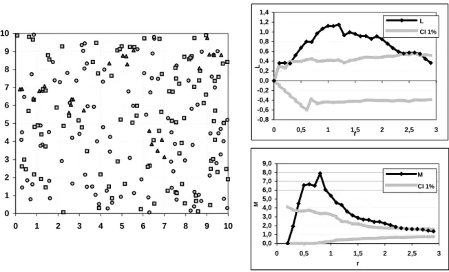
We consider a point set of three different kinds. The first two subsets (squares and circles) are made of 100 points completely randomly distributed. The last (triangles) is generated by a Neyman-Scott process: 5 aggregates (radius 0.5) of 5 points. Every point weight equals 1. The map is in Figure 1, the curves are in Figure 2.

0 1 2 3 4 5 6 7 8 9 10 0 1 2 3 4 5 6 7 8 9 10 -0,8 -0,6 -0,4 -0,2 0,0 0,2 0,4 0,6 0,8 1,0 1,2 1,4 0 0,5 1 1,5 2 2,5 3 r L L CI 1% 0,0 1,0 2,0 3,0 4,0 5,0 6,0 7,0 8,0 9,0 0 0,5 1 1,5 2 2,5 3 r M M CI 1%

Figure 1: Aggregates, Point map Figure 2: Aggregates, L and M functions for

the aggregated point set

The M curve shape is similar to L’s: positive peaks denote concentration. Nevertheless, while

L peaks approximately correspond to the aggregates’ diameter (Goreaud (2000)), M peaks

occur at distances at which the local density is the greatest, that is approximately the distance between points in the aggregates.

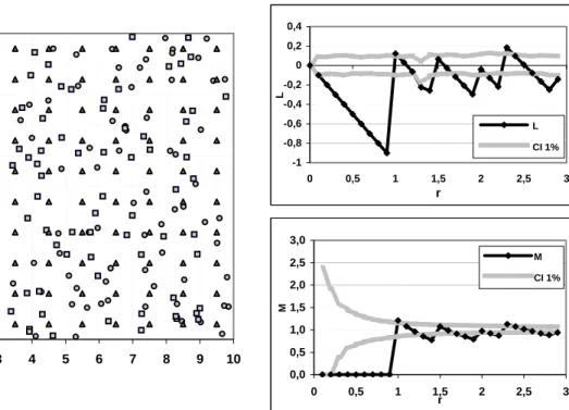
We consider a point set made of three different point types. The first two of them (squares and circles) are constituted of 100 completely randomly distributed points. The last one (triangles) is a perfectly even distribution of 100 points located on a square, 1 by 1 grid. All points’ weights equal 1.

The first part of the M curve is made of 0 values, showing the absence of neighbours at any distance smaller than the grid size. Note that the L curve shape is different since its original value is 0 and its minimum slope is -1 by construction.

At the grid size, M value suddenly increases (the curve continuity is actually an artefact due to interpolation between points). It decreases again between each point-to-point distance ( 2 ≈1,44 is the diagonal length, then 2, 5 ≈2,24 and so on).

Regularity 0 1 2 3 4 5 6 7 8 9 10 0 1 2 3 4 5 6 7 8 9 10 -1 -0,8 -0,6 -0,4 -0,2 0 0,2 0,4 0 0,5 1 1,5 2 2,5 3 r L L CI 1% 0,0 0,5 1,0 1,5 2,0 2,5 3,0 0 0,5 1 1,5 2 2,5 3 r M M CI 1%

Figure 3: Regular point set, Map point Figure 4: Regular point set, L and M functions for the regular point set

Inhomogeneous point set

We generated two completely random point sets (squares and circles) in a 10-by-10 domain.

0 10 20 30 40 50 60 70 0 10 20 30 40 50 60 70 -1,0 -0,5 0,0 0,5 1,0 1,5 2,0 2,5 3,0 0 0,5 1 1,5 2 2,5 3 r L L CI 1% 0,0 0,5 1,0 1,5 2,0 2,5 0 0,5 1 1,5 2 2,5 3 r M M CI 1%

Figure 5: Inhomogeneous point set, Point map Figure 6: Inhomogeneous point set, L and M functions

Then, we transformed the points’ coordinates: after having calculated the polar coordinates (r,θ) of each point from the centre of the point set, we squared the distance to get (r²,θ). The result is a non-homogeneous Poisson pattern, in Figure 5. Both point types have the same random distribution, but the centre of the map shows a greater density, this pattern can be compared with a plants distribution around an industrial centre.

The L function is not applicable: assuming homogeneity, it will interpret the point distribution

as a single big aggregate.

The M function is able to control for density variations. Figure 6 shows the M values for the

first point kind: since its pattern does not differ from the other, its value is around 1.

6.2 Empirical examples

We retained two concrete examples of applications of the M function computed from real data

in two different fields: spatial economics and geographical epidemiology. Hereinafter, weighted points are considered.

Evaluating the geographic concentration of industries

The first example is taken from Marcon and Puech (2003b)7. In this article, the location pattern of French manufacturing firms located in the whole metropolitan France in 1996 is

studied. The sample is composed of more than 36,000 firms in fourteen sectors of activity. Every firm is weighted by its number of employees. In this case, the M function allows

measuring the industrial concentration in France for a specific sector (intra-industry concentration).

In every manufacturing sector, significant concentration is detected. However, three main conclusions can be drawn. Firstly, the degree of industrial concentration measured by the M

function noticeably differs from an industry to another. Secondly, the maximum concentration (significant concentration peak) does not appear at the same distance for each industry (the maximum concentration occurs at small distances, i.e., in a radius of a few kilometres). And

finally, the range of distances, on which an over-representation of the sector of activity compared to the whole area is significant, clearly varies across industries.

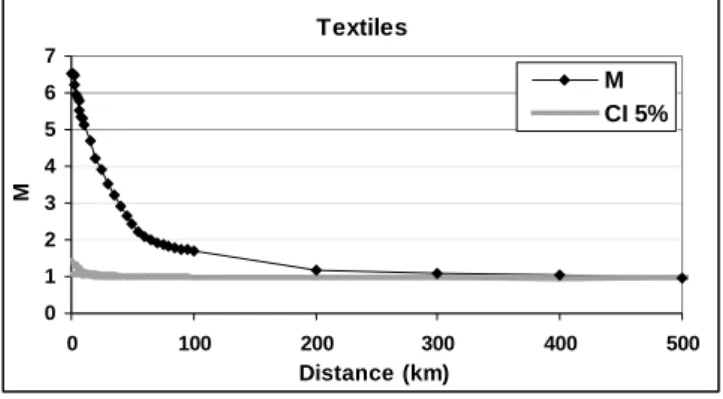
As an example, Figure 7 illustrates M function results for textiles (sector for which the highest

peak is detected). The confidence interval is computed at a 5% confidence level from 20 simulations only, due to computing time and considering the clearness of the departure from the null hypothesis. Significant concentration is observed up to 200 kilometres. The peak reaches around 6.5 at a radius less than 1 kilometre.

Textiles 0 1 2 3 4 5 6 7 0 100 200 300 400 500 Distance (km) M M CI 5%

Figure 7: M function for textiles in France

7

This indicates that at this radius, the relative density of employees in textiles is more than six times greater around textiles firms than in the whole area. It is worth noting that, in spatial economics, using distance-based methods like Ripley’s K is quite new and cluster-based

methods are more widely employed to evaluate the spatial agglomeration of the economic activity.

Cuzick and Edwards (1990) data set

Cuzick and Edwards (1990) introduced the first formal way to deal with non-homogeneous point processes. They used a data set (published with the paper) concerning the location of 62 cases of childhood leukaemia between 1974 and 1986 in the North Humberside area, England. A control set of 141 children representing the whole concerned population was chosen from the birth register. They could conclude that the cases were significantly clumped. We use this data set to go further. We are now able to corroborate their conclusion and also to precise the size of the aggregates.

420 430 440 450 460 470 480 470 480 490 500 510 520 530 540 -150 -100 -50 0 50 100 150 0 0,5 1 1,5 2 Distance (Km ) D D CI 10% 0 0,5 1 1,5 2 0 0,5 1 1,5 2 Distance (Km ) M M CI 10%

Figure 8: Childhood Leukemia map Figure 9: Cuzick and Edwards (1990) point set,

D and M functions

The map is in Figure 8, cases are represented by circles and controls by crosses. Figure 9 shows M values for the cases. Note that it was computed according to the case-control design,

equation (26). We can confirm clumping and precise it: in a 0.7 km radius around a case, the average case density is about 70% higher than it would be if the cases followed the control pattern (at this distance, the peak of the M function reaches 1.7).

In the discussion of Cuzick and Edwards (1990), Diggle (p.101) suggested that the D

function, equal to Kcases-Kcontrols, would lead better results. The next year Diggle and

Chetwynd (1991) published the mathematical framework of the D function and computed

their new function on the same dataset. In figure 9, we recomputed D (considering the

Cases

Case

rectangle domain shown in Figure 88) and estimated the M function. It can be seen that the M

and D functions give the same results if points are not weighted. Nevertheless, D values can

not be interpreted easily and not compared across distances.

Both methods suffer here from a severe lack of power due to the very little number of controls. The confidence intervals are computed at 5% and 10% levels (from 1000 simulations). Increasing the number of controls would not have been a real problem if the experimental design had included a distance-based point pattern analyse.

7 Conclusion

The M function is defined as a generalization of Ripley’s K function to allow its application to

inhomogeneous point processes and to take into account point weights.

We had to reformulate the K function to understand it as a probability ratio, and by the way

correct a bias remained in its definition despite occasional attempts to eliminate it. We also had to choose a definitive edge-effect correction method to make the whole theory consistent. The probabilistic approach allows considering spatial heterogeneity. When using the K

function, we know, or at least we hope, that the point process is stationary, i.e. the probability

to find a neighbour scales with the area. However, using the M function, we suppose that the

probability to find a neighbour of the good kind is given by the average proportion of good-kind neighbours combined with the local density of points. This assumption is very general and holds in most cases. Yet, this is an assumption and must be clearly kept in mind.

We think this is a significant improvement for spatial structure analysis:

• First of all because the number of situations in which the spatial structure can be analysed will dramatically increase (unfortunately, inhomogeneous point processes are not uncommon) if we compare it to the possible applications of K.

• M is more powerful than D because it does not ignore a part of the data.

• M is more convenient to use than K because no edge-effect correction is required. More than this, the domain limits do not have to be known, the point locations are enough. Therefore, complete geographical data sets can be treated without simplifying the domain shape and eliminating many border points.

• M does not require a good knowledge of the underlying point process and a pre-computation of local densities like Kinhom does.

• Neither K nor D nor Kinhom take into account the points’ weight.

To allow effective use of the M function, we developed the necessary software, available on

the authors’ web site9.

8

Note that this data set was widely used and gave slightly different results according to the domain definition in Diggle and Chetwynd (1991), p. 1160, or Rowlingson and Diggle (1993), p. 634

9

References

Baddeley, A. J., Møller, J. and Waagepetersen, R. (2000). "Non- and semi-parametric

estimation of interaction in inhomogeneous point patterns." Statistica Neerlandica

54(3): 329-350.

Besag, J. E. (1977). "Comments on Ripley's paper." Journal of the Royal Statistical Society B

39(2): 193-195.

Clark, P. J. and Evans, F. C. (1954). "Distance to nearest neighbor as a measure of spatial

relationships in populations." Ecology 35(4): 445-453.

Cressie, N. A. (1993). Statistics for spatial data. John Wiley & Sons, New York. 900 p.

Cuzick, J. and Edwards, R. (1990). "Spatial Clustering for Inhomogeneous Populations."

Journal of the Royal Statistical Society B 52(1): 73-104.

Diggle, P. J. (1983). Statistical analysis of spatial point patterns. Academic Press, London.

148 p.

Diggle, P. J. (1985). "A Kernel Method for Smoothing Point Process Data." Applied Statistics

34(2): 138-147.

Diggle, P. J. and Chetwynd, A. G. (1991). "Second-Order Analysis of Spatial Clustering for

Inhomogeneous Populations." Biometrics 47: 1155-1163.

Feser, E. J. and Sweeney, S. H. (2000). "A test for the coincident economic and spatial

clustering of business enterprises." Journal of Geographical Systems 2(4): 349-373.

Gatrell, A. C. and Bailey, T. C. (1996). "Interactive Spatial Data Analysis in Medical

Geography." Social Science & Medicine 42(6): 843-855.

Gatrell, A. C., Bailey, T. C., Diggle, P. J. and Rowlingson, B. S. (1996). "Spatial point

pattern analysis and its application in geographical epidemiology." Transactions of the Institute of British Geographers 21: 256-274.

Getis, A. (1984). "Interaction modeling using second-order analysis." Environment and

Planning A. 16: 173-183.

Getis, A. and Franklin, J. (1987). "Second-order neighborhood analysis of mapped point

patterns." Ecology 68: 473-477.

Goreaud, F. (2000). Apports de l'analyse de la structure spatiale en forêt tempérée à l'étude

de la modélisation des peuplements complexes. Thèse de doctorat, ENGREF. Nancy.

Goreaud, F. and Pélissier, R. (1999). "On explicit formulas of edge-effect correction for

Ripley’s K-function." Journal of Vegetation Science 10(3): 433-438.

Haase, P. (1995). "Spatial pattern analysis in ecology based on Ripley's K function:

Introduction and methods of edge correction." Journal of Vegetation Science 6(4):

575-582.

Jones, A. P., Langford, I. H. and Bentham, G. (1996). "The Application of K-Function

Analysis to the Geographical Distribution of Road Traffic Accident Outcomes in Norfolk, England." Social Science & Medicine 42(6): 879-885.

Kingham, S. P., Gatrell, A. C. and Rowlingson, B. S. (1995). "Testing for Clustering of Health Events within a Geographical Information System Framework." Environment and Planning A. 27(5): 809-821.

Kuuluvainen, T. and Rouvinen, S. (2000). "Post-fire understorey regeneration in boreal

Pinus sylvestris forest sites with different fire histories." Journal of Vegetation Science

11(6): 801-812.

Marcon, E. and Puech, F. (2003a). "Evaluating the Geographic Concentration of Industries

Using Distance-Based Methods." Journal of Economic Geography 3(4): 409-428.

Marcon, E. and Puech, F. (2003b). Measures of the Geographic Concentration of

Industries: Improving Distance-Based Methods. Cahiers de la MSE, 2003.18: 22 p.

Moeur, M. (1993). "Characterizing spatial patterns of trees using stem-mapped data." Forest Science 39(4): 756-775.

Pancer-Koteja, E., Szwagrzyk, J. and Bodziarczyk, J. (1998). "Small-scale spatial pattern

and size structure of Rubus hirtus in a canopy gap." Journal of Vegetation Science

9(6): 755-762.

Peterson, C. J. and Squiers, E. R. (1995). "An Unexpected Change in Spatial Pattern Across

10 Years in an Aspen-White Pine Forest." Journal of Ecology 83(5): 847-855.

Ripley, B. D. (1976). "The Second-Order Analysis of Stationary Point Processes." Journal of Applied Probability 13: 255-266.

Ripley, B. D. (1977). "Modelling Spatial Patterns." Journal of the Royal Statistical Society B

39(2): 172-212.

Ripley, B. D. (1979). "Tests of 'randomness' for spatial point patterns." Journal of the Royal Statistical Society B 41(3): 368-374.

Ripley, B. D. (1981). Spatial statistics. John Wiley & Sons, New York. 255 p.

Rowlingson, B. S. and Diggle, P. J. (1993). "SPLANCS: Spatial Point Pattern Analysis Code

in S-Plus." Computers & Geosciences 19(5): 627-655.

Silverman, B. W. (1986). Density estimation for statistics and data analysis. Chapman and

Hall. 175 p.

Stoyan, D., Kendal, W. S. and Mecke, J. (1987). Stochastic Geometry and its Applications.

John Wiley & Sons, New York. 345 p.

Sweeney, S. H. and Feser, E. J. (1998). "Plant Size and Clustering of Manufacturing

Activity." Geographical Analysis 30(1): 45-64.

Szwagrzyk, J. and Czerwczak, M. (1993). "Spatial patterns of trees in natural forests of

East-Central Europe." Journal of Vegetation Science 4(4): 469-476.

Thioulouse, J., Chessel, D., Dolédec, S. and Olivier, J.-M. (1997). "ADE-4: a multivariate

analysis and graphical display software." Statistics and Computing 7(1): 75-83.

Upton, G. J. G. and Fingleton, B. (1985). Spatial Data Analysis by Example, volume 1:

Point Pattern and Quantitative Data. John Wiley & Sons, New York. 410 p.

Ward, J. S. and Ferrandino, F. J. (1999). "New derivation reduces bias and increases power