Benchmark characterization for reusable launch vehicle onboard trajectory generation using a Legendre psuedospectral [sic] optimization method

Benchmark Characterization for Reusable Launch Vehicle Onboard

Trajectory Generation using a Legendre Pseudospectral Optimization

Method

Theodore R. Dyckman B.S. Aerospace Engineering United States Naval Academy, 2000

SUBMITTED TO THE DEPARTMENT OF AERONAUTICS AND ASTRONAUTICS IN PARTIAL FULFILLMENT OF THE REQUIREMENTS FOR THE DEGREE OF

MASTER OF SCIENCE IN AERONAUTICS AND ASTRONAUTICS AT THE

MASSACHUSETTS INSTITUTE OF TECHNOLOGY JUNE 2002

0 2002 Theodore R. Dyckman. All Rights Reserved.

The author hereby grants to MIT permission to reproduce and to distribute publicly paper and electronic copies of this thesis document in whole or in part.

Signature of Author

i-"Department of Aeronautics and Astronautics May 24, 2002 Certified by

Gregg H. Barton Next Generation Guidance & Control Principle Investigator The Charles Stark Draper Laboratory, Inc.

SrTechnical Supervisor

Certified by

John J. Deyst Professor of Aeronautics and Astronautics Thesis Advisor

/i /I A

Accepted by

Wallace E. Vander Velde Professor of Aeronautics and Astronautics

MASSACHUSETTS ISTITUTE Chair, Committee on Graduate Students OF TECHNOLOGY

-4

Benchmark Characterization for Reusable Launch Vehicle Onboard Trajectory Generation using a Legendre Pseudospectral Optimization Method

by

Theodore R. Dyckman

Submitted to the Department of Aeronautics and Astronautics on May 24, 2002, in partial fulfillment of the requirements for the

Degree of Master of Science in Aeronautics and Astronautics

Abstract

Draper Laboratory has developed a core technology that provides the foundation for onboard trajectory generators. The main goal is for these generators to create robust trajectories for the Terminal Area Energy Management phase of flight. The current onboard generator is the first working prototype that utilizes this core technology and has demonstrated the design of multiple trajectories for varying conditions. However, the optimality or robustness of these trajectories is not known. Therefore, in order to further progress the work done in real-time trajectory generation, it is necessary to establish the metrics for determining the robustness of a trajectory. This will also help in the creation of a suitable benchmark for which to judge and formulate future trajectory generators. This thesis determines benchmark robust trajectories for the current onboard trajectory generator. This is accomplished by utilizing an optimization routine to generate a wide variety of trajectories around different cost functions. A physical measure and definition of robustness was then determined through a thorough analysis of all the parameters of the optimized trajectories. This led to the selection of a benchmark cost function that portrays the definitive characteristics of robust trajectories. In addition, the grading system used in the determination of the benchmark can be used to calculate a quantitative value of robustness for existing trajectories.

The robustness grading system, along with analysis of different trajectories, led to the characterization of the trajectories created from the current onboard generator. While these trajectories were determined to be solutions to tightly constrained problems, they also proved to be sub-optimal representations of the trajectory benchmark. In addition, they are shown to be fairly robust as well. Information and insight gained in the thesis is used to present recommendations for ways to continue the development and testing of new technology for onboard trajectory generation.

Technical Supervisor: Gregg H. Barton

Title: Principle Member of the Technical Staff, C.S. Draper Laboratory, Inc. Thesis Advisor: John J. Deyst

ACKNOWLEDGMENT May 24, 2002

Foremost, I would like to thank the Charles Stark Draper Laboratory for providing the opportunity, funding, and support necessary to pursue my graduate education at MIT. I am extremely grateful for all the help and guidance that was given to me by members of the staff, including Anil Rao, Ron Proulx, and Chris D'Souza for helping with optimization and any DIDO questions. Particular thanks goes especially to my technical advisor, Gregg Barton, for guiding, teaching, and helping me through this entire process. It is hard to believe this thesis has come so far, especially since we were both very nervous at how it was going to go, not to mention how we were going to tackle the problem we did. I can't say I truly enjoyed laying plot upon plot on your desk, but it was fun at times. Luckily all the chips fell in to place, and not a moment too soon, or too late for that matter. Thanks again.

Second, I would like to express my appreciation to the staff and professors in the MIT Aeronautics and Astronautics Department. Particular thanks go to my thesis advisor, Professor John Deyst, for his time, effort and support. I also enjoyed your Real-Time systems class. It was tough, but I learned a lot. Thanks.

Next, I thank my friends and fellow Draper fellows who have kept me both distracted and focused during these past two years. To the first group of fellows, Steve, Rich, and Raja, for letting me join you for lunch everyday. Raja, thanks for introducing me to the MIT and Draper ways, in addition to the heads up about Vance AFB. I sure you would like to know that the plant is doing well. To Andrew, the only other Navy guy at the time, thanks for your help on how to write the thesis, not to mention the actual template to follow. Also, thanks to Paul for help with MATLAB basics. To the second group of fellows, Geoff, Kim, Christine, Dave, and Jen, its been interesting. It was such a change to have so many new students, and to have to take up a few tables for lunch. To Stuart, for helping with the repotting of the plant, and for being my office mate until you were booted, although you still came in and chatted all the time. Thanks for reminding me to start writing, and see... .I did finish it. To Steve, man those workouts are a pain in the butt. Thanks for helping me give a strong showing for the Navy, and for all the good times. Sorry about introducing you to the drive you have to make next year, although Marblehead is awesome. Thanks to Rob and Andy; you got to love those bi-weekly presentations.

Finally, I want to thank my family for their love, support, encouragement and guidance. I am sure you got sick of all my phone calls and complaints, but don't worry, I am sure you will hear it from flight school. I would not be where I am right now if it wasn't for all of you. Thank you so much.

This thesis was prepared at The Charles Stark Draper Laboratory, Inc., under Next Generation Guidance and Control, Internal Research and Development project #18544. Publication of this thesis does not constitute approval by Draper or the sponsoring agency of the findings or conclusions contained herein. It is published for the exchange and stimulation of ideas.

Table of Contents

3.2 Reference Coordinate Fram es ... 31

3.3 Transform ation of Coordinate Fram es ... 32

3.4 N onlinear Equations of M otion... 35

4 G uidance and Control... 43

4.1 O verview ... 43

4.2 Traditional Shuttle Guidance and Control ... 43

4.2.1 Guidance and Control Concept ... 43

4.2.2 Terminal Area Energy Management and Approach and Landing Phases... 45

4.2.3 Lim itations... 49

4.3 N ext Generation Guidance and Control (N GG C)... 51

4.3.1 Guidance and Control Concept ... 51

4.3.2 Com ponents... 51

5 Onboard Trajectory Generation ... 55

5.1 Overview ... 55

5.2 K ernel Extraction Protocol (KEP)... 55

5.2.1 K ernel Equations of M otion... 55

5.3 Geom etrically Constrained M ethods... 62

5.3.1 Definition... 62

5.3.2 Auto-Landing I-load Program (ALIP) ... 63

5.3.3 ALIP3D ... 65

5.3.4 Lim itations... 68

5.4 Sub-optimal Nodal Application of the Kernel Extraction (SNAKE) Method ... 70

5.4.1 Overview ... 70

5.4.2 Dynam ic Pressure Schedule... 71

5.4.3 Ground Track Formulation ... 75

5.4.4 Rapid Trajectory Propagation ... 79

5.5 Proto-Snake ... 81

5.5.1 M ethodology ... 81

5.5.2 Lim itations... 84

5.6 Sum m ary ... 85

6 Optim ization Tools... 87

6.1 Overview ... 87

6.2 Optim ization Problem ... 87

6.3 Optim ization M ethods... 89

6.3.1 Pseudospectral M ethods ... 89

6.3.1.1 Finite Difference M atrix... 89

6.3.1.2 Pseudospectral Differentiation M atrix ... 91

6.3.2 Legendre Pseudospectral Optim ization M ethod ... 93

6.4 Direct Indirect Dynam ic Optim ization (DIDO) ... 94

6.5 Software and Hardware Specifications ... 95

6.5.1 Software... 95

6.5.2 Hardw are ... 96

7 Benchm ark Determ ination ... 97

7.1 Overview ... 97

7.2 Problem Setup ... 97

7.2.1 M athem atical Form ulation ... 97

7.2.1.2 Dynam ic Constraints ... 98

7.2.1.3 Event Constraints ... 99

7.2.1.4 Path Constraints... 100

7.2.2 N on-Dim ensionalization ... 101

7.2.3 Tables ... 103

7.2.4 Nodal Determ ination ... 104

7.2.5 Soft Knot ... 104

7.3 Cost Function Form ulation... 105

7.3.1 Proto-Snake Characterization and Verification... 105

7.3.2 Robust Trajectories... 108

7.3.2.1 Goals... 108

7.3.2.2 Cost Layout ... 109

7.4 Trajectory Selection / Benchm ark Selection... 111

7.4.1 Desirability Criterion... 111 7.4.2 Test Layout... 112 7.4.3 Scoring / Grading ... 120 8 Results ... 129 8.1 Overview ... 129 8.2 Proto-Snake Characterization... 129

8.3 Benchm ark Trajectory / Cost Function ... 133

8.4 Sum m ary ... 140

9 Conclusions ... 143

9.1 Sum m ary and Conclusions... 143

9.2 Recom m endations for Future W ork... 145

Appendix A DIDO Problem Setup... 151

A.1 User Interface Code... 151

Appendix B DIDO Results... 157

B.1 Graphical Presentation of DIDO Results... 157

Appendix C Scoring Results ... 187

C.1 Tables of Param eter Scores ... 187

List of Figures

Figure 2.1: Trimmed Lift and Drag Coefficient (X-34)... 26

Figure 2.2: Trimmed L/D versus Angle of Attack (X-34)... 27

Figure 2.3: Schematic of Orbital Sciences' X-34 [1]... 29

Figure 3.1: Inertial, Local Horizontal and Body Reference Frames ... 32

Figure 3.2: Heading Angle / Flight Path Angle Rotation... 33

Figure 3.3: Bank A ngle Rotation: ... 34

Figure 3.4: Stability and Body Reference Frames ... 35

Figure 3.5: Forces Projected onto the Vertical Plane of the Velocity Reference Frame ... 38

Figure 3.6: Forces Projected onto the Horizontal Plane of the Velocity Reference Frame. 39 Figure 4.1: Traditional Space Shuttle G&C Layout... 44

Figure 4.2: Traditional Approach to Trajectory Generation [7]... 44

Figure 4.3: TA EM Subphases [9] ... 46

Figure 4.4: Acquisition Subphase Segments... 47

Figure 4.5: Flight Path along the HAC [9]... 48

Figure 4.6: Approach and Landing Subphases [9]... 49

Figure 4.7: Next Generation Guidance and Control System Concept ... 51

Figure 4.8: NGGC Approach to Onboard Trajectory Generation [7]... 52

Figure 5.1: "Balancing the Dynamics" through Dynamic Pressure... 61

Figure 5.2: Auto-Landing Subphases and Geometry [11] ... 63

Figure 5.3: Effect of Adjusting XZERO [11] ---... 65

Figure 5.4: Elements of Lateral Geometry [13]... 66

Figure 5.5: Elements of Longitudinal Geometry [13]... 67

Figure 5.6: Possible High Mach Number Acquisition Turn [1]... 69

Figure 5.7: ALI-relative Coordinate System [1]... 70

Figure 5.8: Dynamic Pressure Schedules... 72

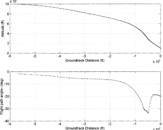
Figure 5.9: Flight Path for Max Dive Trajectory ... 73

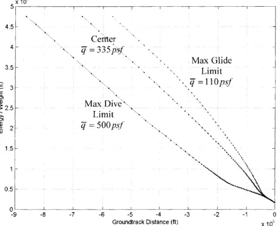
Figure 5.10: Typical Energy Corridor... 74

Figure 5.12: Ground Track Segment Orientation [1]... 76

Figure 5.13: Family of Constant Nz Turns [1]... 77

Figure 5.14: Analogy of Toy Snake to Ground Track [1]... 78

Figure 5.15: Manipulation of Projected Ground Track to the ALI [1] ... 79

Figure 5.16: General Propagation Algorithm [I]... 80

Figure 5.17: y versus %, Table for Segment Length Prediction [1]... 82

Figure 5.18: Phase One of the Ground Track Solver [1] ... 83

Figure 5.19: Phase Two of the Ground Track Solver [I]... 83

Figure 6.1: Position Data Taken at LGL Time Points [16]... 93

Figure 7.1: Comparison of DIDO Verification Trajectory to a Proto-snake Trajectory... 107

Figure 7.2: Proto-snake Reference Trajectories... 114

Figure 7.3: Effect of

a

A

Figure 7.4: Effect of

a

Figure 7.5: Comparison of Different Dynamic Pressure Profiles ... 119

Figure 7.6: Dynamic Pressure Scoring Scheme ... 122

Figure 7.7: Nzb Scoring Scheme... 123

Figure 7.8: Heading Angle Scoring Scheme... 124

Figure 7.9: Crossrange Parameter Scoring Area... 125

Figure 7.10: Crossrange Parameter Scoring Scheme ... 126

Figure 7.11:

a

A

Figure 8.1: Effect of y Parameter in Cost Function... 130

Figure 8.2: Nzb Parameter Matching Issue ... 131

Figure 8.3: Comparison of (qam) Trajectories with Proto-snake... 132

Figure 8.4: Most Robust Trajectory of Point 1 ... 134

Figure 8.5: Most Robust Trajectory of Point 2 ... 136

Figure 8.6: Most Robust Trajectory of Point 3 ... 137

Figure 8.7: Most Robust Trajectory of Point 4 ... 139

Figure 9.1: Dynamic Pressure Schedule Plateaus ... 146

Figure 9.2: "Steer-to-Zero" Logic ... 148

Figure 9.3: "Steer-to-Transition" Logic ... 149

DIDO DIDO DIDO DIDO DIDO DIDO DIDO DIDO

Run (qamyl) versus Point 1 Reference ... Run (qamc l) versus Point 1 Reference... Run (minEamnzl) versus Point 1 Reference ... Run (minEamyl) versus Point 1 Reference... Run (maxEamc 1) versus Point 1 Reference ... Run (maxEamyl) versus Point 1 Reference ... Run (qam2) versus Point 2 Reference ... Run (qamy2) versus Point 2 Reference ...

Figure B.10: DIDO Run (qamc2) versus Point 21 Reference... 167 Figure B.11: Figure B.12: Figure B.13: Figure B.14: Figure B.15: Figure B.16: Figure B.17: Figure B.18: Figure B.19: Figure B.20: Figure B.21: Figure B.22: Figure B.23: Figure B.24: Figure B.25: Figure B.26: Figure B.27: Figure B.28:

DIDO Run (minEamnz2) versus Point 2 Reference ... DIDO Run (minEamy2) versus Point 2 Reference ... DIDO Run (maxEamc2) versus Point 2 Reference ... DIDO Run (maxEamy2) versus Point 2 Reference ... DIDO Run (qam3) versus Point 3 Reference... DIDO Run (qamy3) versus Point 3 Reference... DIDO Run (qamc3) versus Point 3 Reference... DIDO Run (minEamnz3) versus Point 3 Reference ... DIDO Run (minEamy3) versus Point 3 Reference ... DIDO Run (maxEamc3) versus Point 3 Reference ... DIDO Run (maxEamy3) versus Point 3 Reference ... DIDO Run (qam4) versus Point 4 Reference... DIDO Run (qamy4) versus Point 4 Reference... DIDO Run (qamc4) versus Point 4 Reference... DIDO Run (minEamnz4) versus Point 4 Reference ... DIDO Run (minEamy4) versus Point 4 Reference ... DIDO Run (maxEamc4) versus Point 4 Reference ... DIDO Run (maxEamy4) versus Point 4 Reference ... Figure Figure Figure Figure Figure Figure Figure Figure B.2: B.3: B.4: B.5: B.6: B.7: B.8: B.9: 159 160 161 162 163 164 165 166 168 169 170 171 172 173 174 175 176 177 178 179 180 181 182 183 184 185

List of Tables

Table 2.1: X -34 Physical Characteristics [3, 4] ... 29

Table 6.1: Com puter Hardware Specifications ... 96

Table 7.1: Description of State Variables ... 98

Table 7.2: Path Constraint Bounds... 101

Table 7.3: Longitudinal Param eters ... 110

Table 7.4: Lateral Param eters... 110

Table 7.5: Desirability Criterion ... 111

Table 7.6: Center of Corridor Cost Functions... 113

Table 7.7: M ax Glide Cost Functions ... 113

Table 7.8: M ax Dive Cost Functions ... 113

Table 7.9: Initial Conditions of Proto-snake Reference Trajectories... 115

Table 7.10: Cost Functions Remaining After Second Down-Selection... 118

Table 7.11: Cost Functions Remaining After Third Down-Selection... 120

Table 7.12: Benchm ark Selection / Robustness Param eters ... 121

Table 7.13: Scoring Param eter W eightings... 127

Table 8.1: Point 1 Grading Results ... 134

Table 8.2: Point 2 Grading Results ... 136

Table 8.3: Point 3 Grading Results ... 137

Table 8.4: Point 4 Grading Results ... 138

Table 8.5: Overall Grading Results... 139

Table C. 1: Point 1 Trajectory Results ... 187

Table C.2: Point 2 Trajectory Results ... 187

Table C.3: Point 3 Trajectory Results ... 188

List of Symbols

a ... A cceleration

a ... A cceleration vector b ... W ing span

C ... Mean aerodynamic chord

CD ---...-- - - - . Aerodynamic drag coefficient

CG ... Center of gravity

CL---...--- Aerodynamic lift coefficient

D... Aerodynamic drag force

D ... Differentiation matrix e ... Event constraint function

E W... Energy-over-weight ... Total force vector

ro...Aerodynamic force vector

gravit...Gravity force vector

g ... G ravity force

h ... A ltitude

hnorn ... Normalizing altitude value

h* ... N orm alized altitude

Ah ... Small altitude increment (step) kAa ...Adaptive gain for small change in a

L... Aerodynamic lift force

L ... Integrand or Lagrange cost function

L/D ... Lift-over-drag

m ... M ass

M ... M ach num ber

maxEamc ... Cost function maximizing E W and minimizing d,tA, and X

maxEamy ... Cost function maximizing E/W and minimizing

d, A, and y

minEamnz... Cost function minimizing E W, &,Ai, and Nzh

minEamy... Cost function minimizing E W, &, L& and y

Nxb ... Body frame x-acceleration

Nyb ... Body frame y-acceleration

Nx ... Velocity fram e x-acceleration Nyv ... Velocity fram e y-acceleration

Nzv ... Velocity fram e z-accleration p ... Path constraint function

q ... Dynam ic pressure

qam ... Cost function m inim izing (i - 335), a, ,u

qamc ... Cost function m inim izing (q - 335), d, ft, and y qamy ... Cost function m inim izing (i7 - 335), d,

ft,

r ... Position vector S... Planform area

t... Tim e

Ta2b ... Transform ation m atrix from a to b

u...Vector of control variables V ... Inertial (ground-relative) velocity Vnortn...N orm alizing velocity value

V* ... N ormalized velocity

F ... Velocity vector

W ... W eight

x ... Downrange distance (position com ponent)

Xnorn, ... N orm alizing downrange value

x* ... N orm alized downrange distance

x...Vector of state variables

y ... Crossrange distance (position com ponent)

Ynorn ... N orm alizing crossrange value

y* ... N orm alized crossrange distance Y... Side force

z ... Vertical position com ponent

a ... Angle of attack l ... Sideslip angle

s ... Speedbrake position

X ... Runway-relative heading angle $... End point or M ayer cost function

... Roll angle y... Flight path angle p ... Bank angle p ... Density

r ... C lock tim e

S... Initial clock time

T ... Final clock time

List of Acronyms

DIDO... Direct Indirect Dynamic Optimization G&C ... Guidance and Control

GTS ... Ground Track Solver HAC ... Heading Alignment Cone

IG&C... Integrated Guidance and Control KEP ... Kernel Extraction Protocol M D ... M ax D ive

M G ... M ax G lide

NGGC...Next Generation Guidance and Control RLV... Reusable Launch Vehicle

SNAKE... Sub-optimal Nodal Application of Kernel Extraction TAEM... Terminal Area Energy Management

Chapter 1

Introduction

1.1 Background

The flight success of the Space Shuttle is based in part on its re-entry guidance and control algorithms. So much so, that even after 25 years little has been done to improve upon the baseline shuttle Guidance and Control (G&C) framework. Even vehicles being designed today, like the X-34, X-37 and X-40, utilize G&C techniques designed to operate on circa 1970s flight computers. These algorithms were originally restricted by the limited memory and raw computing power available at the time. They rely on loaded trajectories defined well before launch, which involves labor-intensive pre-flight design, restricts the vehicle to tight, nominal flight corridors and reduces the vehicle's robustness to changing flight conditions. Any abort contingencies must also be defined, and pre-loaded, which effectively prevents the full exploitation of a vehicle's recovery capacity. In addition, any flight condition encountered by the vehicle for which no pre-planned trajectory has been defined may result in the catastrophic loss of the vehicle.

The Charles Stark Draper Laboratory (Draper) has begun an initiative to develop the technologies necessary for the formulation of a next generation guidance and control framework for Reusable Launch Vehicles (RLV). This framework seeks to address and improve upon the limitations of the shuttle era G&C systems. The plan calls for three key components: an autonomous abort planner, an onboard trajectory generator and an Integrated G&C (IG&C) framework. Understanding the relationship between these components provides a clearer context for each individual technology.

Current shuttle G&C techniques rely on mission planners designing trajectories for every abort scenario they can envision and loading these "canned" responses into the vehicle's flight computer. While this may prove effective for a small range of conditions, the current system is not capable of robust abort, or the ability to direct the vehicle to a safe landing for a wide range of off-nominal failure conditions. In contrast, an autonomous abort planner would instantaneously assess the vehicle's current states and scrutinize the available "energy versus downrange" for a variety of landing options. It would select the

best runway within the vehicle's capability, but must rely on the guidance system to generate the necessary reference trajectory.

The onboard trajectory generator would autonomously create the reference trajectories from the vehicle's current position to the desired terminal conditions in real time. This could greatly enhance the G&C's capacity to handle off-nominal, anomalous conditions while taking advantage of the vehicle's full flight capability. While its use in this capacity may provide the greatest enhancement for next generation systems, it should also function equally well under nominal flight conditions. The use of an onboard generator will eliminate the need for mission-specific, pre-defined trajectories and can lead to greater robustness, improved overall performance and lower operational costs. In order to fully capture the improvements offered by an onboard trajectory generator, it is necessary to couple it with an IG&C framework. This would enable the control system to utilize the new guidance inputs and recalculate the necessary control gains so that the vehicle accurately follows the reference trajectory. The current shuttle-based techniques separate the G&C functions, which has the undesired result that the guidance and control systems sometimes react to each other instead of cooperating to achieve the desired trajectory. An IG&C framework has the potential to overcome these difficulties by integrating and coupling the guidance and control systems, allowing real-time implementation of onboard generated trajectories and improved performance.

1.2 Problem Definition

Draper's work in pursuit of the onboard trajectory generation component has resulted in the creation of three different programs, all utilizing the X-34 as a representative RLV model. The Auto-Landing I-Load Program (ALIP) was developed by G. H. Barton as a rapid, pre-mission design tool for the generation of autolanding trajectories. This program laid the foundation for rapid, real-time trajectory propagation and served as starting point for further research conducted by A. R. Girerd. In his 2001 MIT Master's thesis, Girerd presented methodologies for onboard generation of trajectories throughout the subsonic portion of the Terminal Area Energy Management (TAEM) flight regime, consisting of altitudes less than 40,000 feet. His results provided the insight for the necessity of a more general design approach, which encompasses the full range of TAEM, including supersonic and high altitude flight. This led to the development of Proto-snake, by A. C. Grubler, which demonstrates a unique trajectory generation

methodology that uses dynamic pressure schedules and a real-time ground track solver. The methodology consists of predicting a straight-line ground track shape, derived from the full capabilities of the vehicle, and then "snaking" around the ground track to satisfy the given design constraints. This solution method enables the program to design trajectories throughout the TAEM regime and for a variety of different vehicle conditions.

Proto-snake does have its limitations however. Currently the ground track solver employed by Proto-snake provides an ad hoc solution for limiting cases, through the use of "brute force" techniques. While this does provide solutions for varying conditions, it does not create optimal trajectories or guarantee robustness*. In addition, the dynamic pressure schedules used in the formulation of the trajectories are user specified. This means that Proto-snake does not choose the best schedule for the given design conditions or present situation.

These limitations are due in part to the lack of a suitable benchmark that represents the defining characteristics of a robust trajectory. These characteristics include the actual lateral ground track shape, in addition to the dynamic pressure schedules flown by the vehicle, which define the longitudinal flight profile of the trajectory. It is hoped that a suitable benchmark will provide characteristics that can be mimicked by a real-time ground track solver to produce sub-optimal robust trajectories for a wide-variety of conditions.

Generating a robust trajectory through offline methods is difficult in itself. While methodologies exist for the propagation of optimal or feasible trajectories, no such program currently generates "robust" trajectories. Optimization routines can be used in the creation of trajectories, however they rely on the formulation of a cost functions that utilize vehicle states and controls. The robustness of a vehicle is not a vehicle state or even a well-defined vehicle parameter. This limits the ability to create benchmark robust trajectories, while at the same time provides freedom for a designer to establish his or her own set of characteristics for defining robust trajectories.

A robust trajectory is defined as a trajectory that can handle future dispersions while still providing the means for the vehicle to attain the final end condition.

1.3 Thesis Objective

This thesis seeks to determine benchmark robust trajectories for the current onboard trajectory generators. This is done by utilizing a Legendre Pseudospectral Optimization method to generate a wide variety of trajectories around different cost functions. An analysis of the resulting trajectories, in addition to the use of desirability criterion, will lead to the determination of the characteristics of robust trajectories. This research also intends to characterize the optimality and robustness of the current trajectories created by A. Grubler's Proto-snake trajectory generator. Furthermore, the resulting trajectories are intended to provide a starting point for the formulation of future ground track solvers. 1.4 Thesis Overview

The present chapter provides an overall view of the main subject of research for this thesis. Subsequent chapters are narrower in their focus as they describe in detail the necessary background as well as procedures for the attainment of the thesis objective. Chapter 2 gives an overview of RLV type vehicles, including the X-34, which was the demonstration vehicle of choice for this research, as well as for previous onboard trajectory generators, while Chapter 3 presents the derivations of the equations of motion, which govern the vehicle in flight. Chapter 4 describes the shuttle-era G&C framework as well as Draper's vision for the Next Generation Guidance and Control (NGGC). The main technological component of Draper's NGGC, onboard trajectory generation, is covered in Chapter 5, including a more thorough description of the three developmental programs and their methodologies. Chapter 6 provides an overview of the Legendre Pseudospectral Method and it use while Chapter 7 describes the actual problem setup used for the determination of a trajectory benchmark. Chapter 8 describes the results of the research program and Chapter 9 concludes the thesis with an overall summation of the results and recommendations for future research.

Chapter 2

Vehicle Description

2.1 Overview

Draper Laboratory has been in pursuit of technologies that are necessary for the formulation of a Next Generation Guidance and Control (NGGC) system for Reusable Launch Vehicles (RLV). In order to understand the development of these technologies, particularly the onboard trajectory generation component, it is necessary to understand the vehicle for which they are designed to guide through the atmosphere. This chapter intends to provide an overview of RLVs in general, including their basic mission design and aerodynamic properties. The last section describes the X-34, which was chosen as the representative RLV model on which the trajectory generation technology was applied during previous research. This thesis continues to use this vehicle for convenience and continuity sake.

2.2 Mission Design

Reusable Launch Vehicles are spacecraft designed to perform specified missions, multiple times. The missions may include ferrying humans and supplies to orbit, launching satellites, or even performing experiments during flight. They were originally developed to dramatically reduce the cost of access to low Earth orbit, strictly due to their reusability. For instance, the Saturn V rocket was expended while sending humans to the Moon. In order to perform another Moon flight, it was necessary to construct another rocket. On the other hand, the Space Shuttle, the first reusable launch vehicle or first generation RLV, has performed over one hundred missions between four flight vehicles.

Draper Laboratory's NGGC concept is primarily focused on guiding shuttle-like RLVs. This includes vehicles designed with the same general characteristics of the Space Shuttle, in addition to the same relative flight dynamics. The shuttle is designed to make unpowered gliding approaches to horizontal landings on a conventional runway. Its general characteristics include low aspect ratio wings, a lifting body shape, and four primary flight control surfaces. The shuttle is also a low Lift-over-Drag (L/D) flight vehicle, and its corresponding trajectories are significantly different from gliding aircraft

or sailplanes. The X-33, X-34, X-37, and X-40 all fall into the category of "shuttle-like" and the NGGC system being developed can easily be applied to any of these vehicles.

2.3 Aerodynamic Properties

Shuttle-class gliding reentry vehicles fly differently from conventional aircraft. With no available thrust to provide a net positive energy source, low L/D vehicles must budget their total energy throughout their entire descent to ensure they will reach the target runway at the specified dynamic constraints. The low L/D characteristics impede efficient gliding performance and generally result in trajectories with steep equilibrium glide slopes and relatively high velocities. Therefore, shuttle-like RLVs usually have a more limited landing footprint and a smaller margin for trajectory errors than higher L/D vehicles. This fact helps to justify the need to design robust trajectories in order to guarantee vehicle safety and recoverability.

-0.5 Maclg 0.7 Attack-(deg) 0 !5 0 -0.4 -0.5 -0 2 4 6 8 10 12 14 16 18 20

Angle of Attack (deg)

0.5u 2 i i a D i (-4

0.4-0 0.3 -

--0

0 2 4 6 8 10 12 14 16 18 20

Angle of Attack (deg)

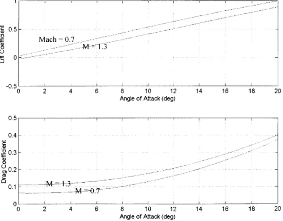
A RLV can control its L/D ratio to some extent by varying its angle of attack, a. This is due to a's effect on the lift and drag coefficients of the vehicle, as shown in Figure 2.1.

The aerodynamic data presented is for the X-34 with a speedbrake setting of 550, but is

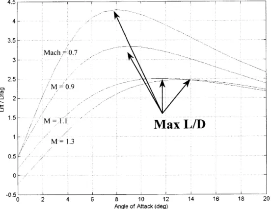
indicative of RLVs in general. For values of a less than five degrees, the lift coefficient varies almost linearly with angle of attack, while the drag coefficient remains relatively flat. Beyond five degrees however, the drag grows exponentially, while the lift retains the linear trend. The resulting L/D curve, shown in Figure 2.2 for various Mach numbers, soon peaks and then starts decreasing. This causes the contour to be divided into afront side and back side. The maximum L/D of the vehicle occurs at the peak in the contour for the given angle of attack. The front side of the curve is usually quite short for low lift-to-drag vehicles such as the shuttle.

4.5 4 3.5 3 2.5 2 1.5 1 0.5 0 0 2 4 6 8 10 12

Angle of Attack (deg)

14 16 18 20

Figure 2.2: Trimmed L/D versus Angle of Attack (X-34)

It is important to keep the L/D curve in mind when designing trajectories. Controllability issues usually mandate keeping the RLV on the front side of the curve, where significant

U Mach 0.7 .ac ... M 0.9 -M-1.1MaxLD M - 13 .......... -- .

changes in lift are accompanied by only modest changes in drag. These characteristics are required to sustain flight at a given flight path angle. If the vehicle flies on the back side of the curve, small changes in lift will result in large drag penalties. As speed is reduced due to the increased drag, the vehicle will try to pitch upward to increase the lift lost by the decrease in speed. This cascades into a non-returnable energy decay wherein a specific trajectory cannot be sustained and may lead to the loss of the vehicle [1].

2.4 Physical Description

The X-34 technology demonstrator, designed by Orbital Sciences, was chosen as the technical model for RLVs in this research. This vehicle was chosen in order to maintain continuity with previous research efforts, which also used the X-34, as well as to take advantage of the large amount of technical information and experience available for the vehicle at Draper Laboratory. Under contract with Orbital, Draper developed the entry and autolanding guidance, as well as the flight software, in support of previously planned flight tests. Also, Draper was awarded a Future-X flight demonstration of autonomous Robust Abort Technologies on the X-34 (RADX34) [2]. However, NASA cancelled the flight tests of the X-34 in April 2001, and the two vehicle specimens are currently in flyable storage. A schematic of the X-34 is presented in Figure 2.3.

The X-34 was developed as a single stage RLV, capable of flights up to 250,000 feet and speeds in excess of Mach 8, after being air-launched from the belly of an L- 1011 carrier aircraft. It was designed to behave similarly to the shuttle in order to minimize risk, cost, and time of development, and even utilizes the same basic flight controls. These include a rudder, speedbrake, body flap and elevons. The body flap is used exclusively as a trim device for successive stages of entry and is not actively employed by the flight control system. All the pertinent physical characteristics of the vehicle are summarized in Table 2.1.

The X-34 is primarily a bank-to-turn vehicle. In its design, the rudder lacks the ability to cause large changes in the vehicle's heading angle and is only used to keep the vehicle in coordinated flight. The vehicle must bank to achieve any desired yaw rate, which results in a slow yaw response due to the need to roll before a change in heading can occur.

The X-34 is also powered by the reusable Fastrac engine, which runs off a mixture of liquid oxygen and kerosene. This was designed and developed by NASA's Marshall Space Flight Center, and can yield approximately 60,000 pounds of thrust. Even though the X-34 is powered, this research is only focused on the unpowered, gliding flight portion of the vehicle's flight envelope.

.UpWsun

-Braking Parachute

Figure 2.3: Schematic of Orbital Sciences' X-34 [1]

Table 2.1: X-34 Physical Characteristics [3, 4]

Length 58.3 feet

Wing Span, b 27.67 feet

Mean Aerodynamic Chord, E 14.54 feet

Planform Area, S 357.5 feet2

Gross Launch Weight 46,500 lbf

Dry Weight 19,000 lbf

Elevon Deflection Range -34.2' to +15.8' Speedbrake Deflection Range 00 to 1030

Chapter 3

Equations of Motion

3.1 Overview

The equations of motion for an atmospheric vehicle are vital to the formulation and the understanding of the developments in this thesis. They are presented in this chapter, along with their derivations and the appropriate assumptions. The first two sections of this chapter describe the necessary coordinate reference frames and the transformation matrices between the frames. The third section covers the derivations of the equations. For more detailed derivations, see References 5 and 6.

3.2 Reference Coordinate Frames

It is necessary to determine a set of coordinate reference frames when formulating the equations of motion for a vehicle. The following five reference coordinate frames are relevant to the movement of a vehicle in atmospheric flight. They all employ right-handed rectangular Cartesian axes.

Inertial Reference Frame (il, , ki): an Earth-fixed coordinate system, with its origin at

the runway threshold as depicted in Figure 3.1. The Earth is assumed to be flat and stationary in inertial space, therefore the Earth is an inertial system, one in which Newton's laws are valid. Additionally, gravity is assumed uniform and constant, and hence the aircraft's center of mass and center of gravity (CG) are the same point.

Local Horizontal Reference Frame (l,, J k,): a coordinate system with the origin at the

vehicle CG, with axes parallel to the inertial reference frame, as shown in Figure 3.1. The rotation matrix between the inertial and local horizontal reference frames is the identity matrix and is time-invariant.

Velocity Reference Frame (l1, J ,,): a coordinate system with the origin at the vehicle

CG and the 1, axis pointing along the velocity vector. The j,, axis remains in the local horizontal i, -

]',

lb >_ l h --Runway b kh kb

---j(Y)

ki

(Z)

Figure 3.1: Inertial, Local Horizontal and Body Reference Frames

Body Reference Frame (i 1,, k,): a coordinate system in which the origin lies at the

vehicle center of gravity. The

l'

Stability Reference Frame (Is, ,J ): a coordinate system with the origin at the vehicle

CG. The i, axis lies along the projection of the velocity vector (V) onto the body

lh

plane. With the assumption of zero sideslip, the velocity vector lies along the is axis. The

f

perpendicular and parallel, respectively, to V and are aligned with the - is and -k, axes

of this frame, as shown in Figure 3.4.

3.3 Transformation of Coordinate Frames

For this thesis, it is assumed that the aircraft always flies coordinated turns. This means that the sideslip angle (p8) is always assumed to be zero. The following transformations take this into account.

Transformations between coordinate frames involve Euler angle rotations about the k, J, and i axes, in order. A transformation matrix (denoted as Ta2b) is a square array containing the Euler rotations between the vector components of the individual coordinate systems. The rotations are represented as sines and cosines of the separation angles between the frames. A vector is rotated from one reference frame into another reference frame by a multiplication of the transformation matrix. Rotating in the opposite direction simply involves multiplying by the transpose of the transformation matrix. Equation 3.1 demonstrates this principle.

y = T,2b Y,

z

h

x

x

L

j

b

z

]

Heading / Flight Path Rotations: The orientation of the velocity reference frame with respect to the inertial and local horizontal reference frames is given by an Euler rotation sequence about the k, and Jh axes as shown in Figure 3.2. In the inertial reference frame, the angles

X

cosysin% cos X sinysing - siny] 0 cosy (3.2) A

Jh

kh

Figure 3.2: Heading Angle / Flight Path Angle Rotation

Bank Angle Rotation: The stability reference frame differs from the velocity reference frame by a bank angle p rotation about their

i

> lIV

- _p

-is ,~b

ks

ki

Figure 3.3: Bank Angle Rotation

1 0 0

Tc = 0 Cos p sin p (3.3)

L0

Angle of Attack Rotation: The transformation from the stability reference frame to the body reference frame is given by a rotation of the angle of attack, a. The angle a is

shown in Figure 3.4 and the transformation matrix is

cosa 0 -sina

TS2b 0 1 0 (3.4)

L

D

ks

Figure 3.4: Stability and Body Reference Frames

Any other required transformation matrices can be expressed as products of those presented above. For example, the transformation matrix from the velocity reference frame to the body reference frame is given by

T 2h =T Ts2T,, (3. 5) simplifying yields sina sin p cos p -cosasin p -sinacosp~ sin p cosacosp_

3.4 Nonlinear Equations of Motion

The full nonlinear equations of motion for an atmospheric vehicle are derived using Newton's Laws. The derivations are subject to assumptions chosen to reduce the complexity of the formulation. These assumptions are listed below.

. the vehicle has a plane of symmetry . the vehicle mass properties are constant

cosa

sina

. the vehicle produces no thrust

. there are no aerodynamic moments (the vehicle is always in a state of static trim) . there are no side forces (Y) present (no sideslip)

. the vehicle is a rigid airframe (no bending) . the wind velocity is always zero

Refer to Reference 1 for derivations that include the complete set of nonlinear wind equations.

The derivation begins by expressing the position vector of the vehicle center of mass with respect to the inertial reference frame, as shown in Eq 3.7. In this frame (as well as the local horizontal reference frame), the positive k,,, axis direction is down. However, this direction refers to the height of the vehicle above ground, and the convention is for a positive increase with vertical distance from the ground. Therefore, the k1, position

component will be expressed as z = -h (where h represents altitude), shown below,

r = xi, + y, + zk, = xl + yjh -hkl, (3.7)

The velocity vector

P

- d

V -- xi11 + jh -hk, _(3.8)

dt

To track the flight path relative to the local horizontal reference frame, it is necessary to transform the velocity vector with respect to the velocity reference frame to the local horizontal reference frame. This is accomplished by using the inverse of the T,2,, matrix.

V

T/=

T,, 0 =VCO Coycos X

i,

The differential equations for the coordinates of the flight path are then

i= VcosycosX

= VcosysinX (3.10)

h= - =V siny

The remaining equations are simply statements of Newton's second law of motion, namely

SF=

The forces affecting the vehicle consist of aerodynamic forces and gravity. The aerodynamic forces are lift (L) and drag (D). The lift and drag vectors represented in these equations are for the complete aircraft, including the wing, tail, fuselage, etc., and act in relation to the stability reference frame of the aircraft. The gravity force, materialized in the weight (W) vector, always acts downward, towards the Earth along the ki,, axis.

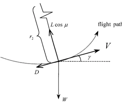
Consider an aircraft CG to be the intersection of the axes of Figure 3.5. The figure is drawn so that the plane of the page is coincident with the i,, -k,, axes of the velocity reference frame. The curvilinear motion of the aircraft along a curved flight path can be expressed by first taking a summation of the forces parallel to the flight path, and then taking a summation of the forces perpendicular to the flight path.

The sum of the forces parallel to the flight path is

S=-D

The acceleration parallel to the flight path is

d

a, =-V=V (3. 13)

L cos p flight path

r2

V

D

SW

Figure 3.5: Forces Projected onto the Vertical Plane of the Velocity Reference Frame

Applying Newton's Law yields

. -D

V= -g siny

m (3. 14)

The components of the forces perpendicular to the flight path are

I F, = W cosy - L cosu (3.15)

The radial acceleration, perpendicular to the flight path, is written in Eq 3.16. It follows the convention of the velocity reference frame, where k, is positive down.

V2

a, = -- - -Vf

where

f

Applying Newton's Law and solving for

f

1

=-

[L

p

mV (3.17)

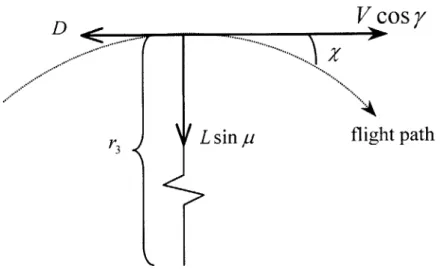
Consider now an aircraft CG to be the intersection of the axes of Figure 3.6. The figure is drawn so that the plane of the page is coincident with the i, - j, axes of the velocity reference frame (top-down view).

D

V cosy

flight path

Lsinp

Figure 3.6: Forces Projected onto the Horizontal Plane of the Velocity Reference Frame

The sum of the forces perpendicular to the flight path is

(3. 18)

Z

The instantaneous radial acceleration along the flight path is

(V cos y)2 _

where -j is the angular velocity equal to the rate of change of the runway-relative heading angle.

Applying Newton's Law and solving for >' yields

L sin p

mrc=sy(3. 20)

m V cos y

The total acceleration vector of the vehicle in the velocity reference frame can be written as a summation of Eqs 3.13, 3.16 and 3.19, as shown below

5a=Vi, + (Vcosy)'j1 -Vfk, (3.21)

The acceleration loading on the vehicle expressed in the body frame is very important. It is a design parameter in certain instances and can be considered a measure of human 'ride-ability' for the vehicle. Specifically, the quantity of interest is the body Nz acceleration. It is defined as the sensed normal specific force or maneuver acceleration of the vehicle along the k, _{axis. To determine the acceleration loading on the vehicle,}

each of the acceleration components are first normalized to gravity.

Nx, = - (3. 22)

g

Ny, = (V cos y) (3.23)

g

NzV = - (3. 24)

Then, the accelerations are rotated from the velocity reference frame into the body reference frame using the transformation matrix in Eq 3.6 to give

Nxh = Nx,cosa + Ny, sin asinp - Nzsina cos p (3. 25)

Nzh = -Nx, sin a+ Ny, cos a sin p - Nz, cos a cos (2

Nzh undergoes a sign change in order to follow the convention whereby positive Nz, is up.

The drag and lift forces contained in the equations can be expressed as functions of the dynamic pressure q7, the vehicle planform area S, and the dimensionless coefficients of lift CL and dragC

L = qSCL

D = qSC)

(3. 28)

(3. 29)

Dynamic pressure can also be written as a function of atmospheric density (which is a function the altitude of the vehicle), and the velocity of the vehicle.

q = pV 2 _{(3. 30)}

Chapter 4

Guidance and Control

4.1 Overview

The purpose of an RLV's Guidance and Control (G&C) system is to guide the vehicle to a safe runway landing without violating certain constraints. These constraints may consist of thermal, dynamic pressure or acceleration loading limits imposed on each trajectory. In the classical arrangement, the guidance system regulates the vehicle's

trajectory and energy, while the flight control system determines the actuator control deflections, based on steering commands from the guidance system. In the case of manned vehicles, including the shuttle, a human pilot typically acts as an intermediary between the guidance and control systems, and interprets cues provided by guidance into commands that are sent to the flight control system. However, future RLV's may be unmanned and will have no pilot available to make up for the limitations in the traditional G&C system layout. These limitations, described in the next section of this chapter, preclude autonomous systems from taking advantage of the full capabilities of the vehicle. Draper Laboratory feels that these limitations can be reduced by the introduction of a new G&C system layout. In order to explain the layout, this chapter first describes the "traditional" shuttle G&C concept and its limitations, and then presents Draper's Next Generation Guidance and Control (NGGC) system.

4.2 Traditional Shuttle Guidance and Control

4.2.1 Guidance and Control Concept

The traditional G&C system concept, including the relationships between various components, is illustrated in Figure 4.1. This concept was originally devised for the Space Shuttle, and due to its proven success, has become the standard for RLVs. Flight planning begins on the ground, by mission planners, who design a series of "reference profiles". These profiles are a set of vehicle states or control histories arranged with respect to some monotonically changing variable, such as time, downrange distance or velocity. The reference profiles are the result of the efforts of engineers to discover, through iterative design and optimization techniques, the nominal and abort trajectories

for a given vehicle mission. A typical profile (or trajectory) design approach used by the engineers is shown in Figure 4.2. Due to any revisions made to a vehicle's aerodynamic characteristics or configuration, and any alterations in expected initial flight conditions, both a nominal trajectory and a series of contingency abort trajectories must be redesigned, and then translated into reference profiles, for each and every flight made by a vehicle. Once the profiles are completed, they are uploaded onto the onboard guidance computers through a large sequence of I-loads, sometimes numbering in the thousands.

On-board

Guidance

---

T-

---

-Fiur 4.1 Trdtoa pc ISuteG Lyu

Figure 4.2: Traditional Approach to Trajectory Generation [7]

Offline

Mission

Design

During a typical flight, the onboard guidance system generates commands that attempt to match the actual vehicle states with the preloaded reference states. These guidance commands are usually for the speedbrake position (8

,h), roll (<), and acceleration along

the vehicle's negative body kb axis (Nz). Once generated, the commands are fed to an

onboard control system that produces a set of deflection commands for the control surface actuators, in the case of an autonomous unmanned vehicle, or a set of pilot cues, in the case of a manned vehicle. It should be noted that in the shuttle-class G&C system, shown in Figure 4.1, the guidance and control systems are artificially partitioned into separate efforts, even though it is a coupled task. Additionally, separate guidance software is required for the nominal flight plan and each abort contingency.

4.2.2 Terminal Area Energy Management and Approach and Landing Phases

Due to the wide variations in conditions that the shuttle, or an RLV, may experience during a typical flight, its entry descent is divided into three sequential phases. This allows the guidance scheme to be broken up into three phases as well, making it more robust than a single scheme developed to handle the entire flight. The three phases are the Entry Phase, the Terminal Area Energy Management (TAEM) Phase, and the Approach and Landing (A/L) Phase. This thesis is only concerned with the flight of RLVs through the TAEM and A/L phases, so only these two areas will be discussed in this sub-section.

The TAEM phase is characterized by glider-type flight dynamics, and is initiated at a specified Mach number and/or altitude where the vehicle attains full control through the use of aerosurfaces only. The purpose of this phase is to control the energy state of the vehicle and direct it towards the landing site. This is accomplished conceptually by flying a predetermined Energy over Weight (E/W) profile as a function of range to the runway, or range-to-go. The E/W term, which captures both the potential and kinetic energies of the vehicle, and thus the total energy, is expressed as:

E =h+ i- (4.1)

During the development of the TAEM phase, engineers decided to split the longitudinal and lateral channels, considering a full integration too complex [8]. Thus, the vehicle's angle of attack controls the longitudinal channel, while the bank angle controls the lateral channel.

The independent variable used during TAEM is range-to-go, and consists of two components: downrange distance and crossrange distance. This variable, more properly defined as the distance left along a predicted ground track, is easily calculated using well-defined geometric segments [9]. For this reason, TAEM is further divided into four distinct subphases, shown in Figure 4.3. These subphases, in order of occurrence, are S-turn, Acquisition, Heading Alignment, and Prefinal Approach. The TAEM phase terminates at a point known as the Auto-Landing Interface (ALI), where the A/L phase begins. 3 Prefinal approchapi subpase Runway

X-G

alignment approach plane

subphaseY

G

Figure 4.3: TAEM Subphases [9]

The S-turn subphase is used to provide large adjustments to the energy state of the vehicle. This subphase is only executed when the vehicle's energy state is too high to reach the ALI at the specified constraints. In other words, the predicted ground track length is not long enough to allow the excess energy to dissipate before reaching the ALI. In such cases, the guidance system commands the vehicle to turn at a maximum rate