Audio denoising using wavelet filter banks aimed at real-time application

(1)

Audio Denoising Using Wavelet

Filter Banks Aimed at Real-Time Application

by

Peter W. Kassakian

B.S., Massachusetts Institute of Technology (1995)

Submitted to the Department of Mechanical Engineering

ENG

in partial fulfillment of the requirements for the degree of MASSACHUSE STITUTE

OFT Y

Master of Science

at the

MASSACHUSETTS INSTITUTE OF TECHNOLOGY

RARIES

June 1999

The author hereby grants to MIT permission to reproduce and distribute publicly paper and electronic copies of this thesis document in whole or in part, and to grant others the right to do so.

Author

Department of Mechanical Engineering May 20, 1999

Certified by

Bernard C. Lesieutre Associate Professor of Electrical Engineering Thesis Supervisor

Certified

by--Derek Rowell Professor of Mechanical Engineering

Thesis Supervisor Accepted by

Ai A. Sonin

(2)

(3)

Audio Denoising Using Wavelet

Filter Banks Aimed at Real-Time Application

by

Peter W. Kassakian

Submitted to the Department of Mechanical Engineering *on May 20, 1999, in partial fulfillment of the

requirements for the degree of Master of Science

Abstract

In this thesis we implement an audio denoising system targeted at real-time application. We investigate the delays associated with wavelet filter bank systems and propose methods to overcome them. We consider computational delays as well as structural delays and deal with each separately. We find that good denoising performance is achieved when filters are chosen so as to transform the input into an appropriately scaled time-frequency domain. Multiplications required for four different implementations of the system are compared and we conclude that a scheme that performs multiplications as far downstream as possible proves to be the best of the four options. Finally we propose several topics for further research including investigations into the human auditory system as well as studies of creative filter bank topologies.

Thesis Supervisor: Bernard C. Lesieutre

Title: Associate Professor of Electrical Engineering

Thesis Supervisor: Derek Rowell

(4)

(5)

Dedication

to

my father

(6)

(7)

Acknow led gements

I would like to express my gratitude to Professor Lesieutre for advising my thesis and taking a

great interest in a topic that's at best tangential to his current research. He made it a pleasure to learn about a subject that is multifaceted and complicated.

Also I want to thank Professor Rowell for reading my thesis on behalf of the department. I'm pleased that he took such an interest in the subject and value his advice on many issues. He also gave me the gift of a very enjoyable TA experience.

I wish to thank Leslie Regan and Joan Kravit for making me feel welcome in their office.

Also thank you very very much, Vivian, Karin, and Sara.

I want to acknowledge Professor Pratt for allowing me to reconsider my involvement in

his project, and for being a kind and caring individual who I will always remember. Professor Verghese deserves special mention too, for his guiding words and insights into these strange filter bank systems.

Finally I want to thank Mom, Meg, Ann, Andrew, and Dennis for their support over the last few years.

(8)

(9)

. . . .

(11)

Contents

A .7 M akefile . . . . 77

B Paraunitary and Unimodular Filters 79

B.1 Paraunitary Filters ... ... 79

(12)

(13)

List of Figures

2.1 A Transform . . . . .. 19

2.2 Signal {1 1} A deterministic signal of length 2 represented as a point on a plane . 21

2.3 Transformed Signal

{v2

0} An orthonormal transformation corresponds to a

rotation of axes. In the above case, the axes are rotated so as to align with the signal point. . . . . 22

2.4 Stochastic Signal of Length 2 A signal specified only by a mean and an

autocor-relation matrix. The ellipses are lines of constant probability. . . . . 23

2.5 Noise Corrupted Musical Signal Represented in Time Domain . . . . 25

2.6 Noise Corrupted Musical Signal Represented in Transform Domain . . . . 26 2.7 Denoised Musical Signal Represented in Transform Domain (Small

Co-efficients Discarded) Here we set a threshold value and remove the smallest coefficients thereby gaining a higher SNR . . . . 26

2.8 Denoised Musical Signal Represented in Time Domain The signal is recon-structed from the thresholded coefficients of Figure 2.7. . . . . 27

3.1 Wavelet Transform Coefficients Plotted Against Time and Frequency Each coefficient can be localized in time and frequency simultaneously. The noise is spread out evenly, and much of it can be removed by setting all the light coefficients to zero. 31

3.2 Time Waveform and Fourier Transform of the Same Signal of Figure 3.1 Although the Fourier transform does give information about the signal of interest (that it has a lot of low-frequency energy), it doesn't show the structure seen in F igure 3.1. . . . . 32

3.3 General Filter Bank A signal of length N can be filtered into M frequency bands, resulting in approximately M x N output samples . . . . 33

3.4 Two Channel Filter Bank with Downsampling The downsampling operator makes it possible to maintain the same number of samples in the transform domain as the time domain. No information is lost if the filters are chosen judiciously. . . . . 34

3.5 Four Channel Filter Bank Tree structures such as these prove to be computa-tionally efficient due to the recursive nature of the tree. . . . . 34

(14)

4.1 Filter Bank Complete with Reconstruction This is a two-channel filter bank. If

no processing is performed, the filters Ho (z), H1 (z), F0 (z), and F1 (z) can be chosen

to perfectly reconstruct x[n], i.e.,

s[n]

= x[n -

1],

where I is the delay in samples.

Larger tree structures can be built from this basic system. . . . 35

4.2 _{Equivalent Polyphase Form of System in Figure 4.1 The polyphase form is} easier to analyze and also faster to implement since the downsampling occurs before the filtering. . . . 36

4.3 Polyphase Analysis Bank . . . 37

4.4 _{Polyphase Analysis Bank (Expanded) . . . 38}

4.5 First Noble Identity in Block Diagram Form . . . 38

4.6 Analysis Bank (Intermediary Form) . . . 38

4.7 _{Analysis Bank (Standard Form) . . . 39}

4.8 _{Construction of a Single Basis Function Here we construct a basis function} by passing one impulse through a reconstruction bank. Four different shapes will be produced, along with their respective shifted versions as seen in Figure 4.9 . . . 40

4.9 Basis Functions of System in Figure 4.8 Notice that there are only four distinct basis function shapes. The total number of basis functions will be equal to the length of the decomposed signal. . . . 41

7.1 Output Sequences for Paraunitary and Unimodular Systems We see that the unimodular system has the striking advantage of possessing very little shift delay. The challenge, however, is to design the filters to be useful . . . 55

(15)

List of Tables

6.1 Multiplications for the Analysis Tree This filter bank has filters of length 30. Note that at each stage, there are more channels, but the signal lengths become shorter, resulting in an almost linear relationship between number of stages and number of multiplies. . . . .. 49

6.2 Multiplications for the Synthesis Tree Notice that there are slightly more multiplies associated with reconstructing the signal than with analyzing it. Also notice that the output signal has been elongated by the approximate length of the basis functions (- 7332). To conserve perfectly the length of the signal throughout

the transform, a circular transform should be taken. . . . . 49

6.3 Multiplications for the Naive Block Causal Analysis Tree Implementation The number of multiplies associated with this transform is extremely high because nothing is precalculated, and multiplications occur as far upstream as possible. . . . 52

(16)

(17)

Chapter 1 Introduction

In this thesis we look at a certain class of systems: wavelet filter bank systems. We are interested in using them in real-time to denoise audio.

The motivation for this work is derived from the desire to use these relatively efficient systems to operate in a setting different from internet related application, where wavelets have gained much attention. Internet compression applications are similar to our denoising system, but do not require a strictly causal system. Our system is geared towards the goal of denoising a piece of audio on the fly, so it could be used quickly in recording situations, or for live performance. This idea sets up an interesting challenge and creates a new angle for viewing these fascinating wavelet systems.

1.1 Organization of Thesis

The thesis is naturally broken into eight chapters, including this one. Chapters 2, 3, and 4 present background material necessary for the understanding of the more subtle discoveries explained in the later chapters. Wavelet systems are different from linear time-invariant systems because they involve a non-time-invariant operator, the downsampler. It's for this reason that these background chapters are included. The three chapters provide a self-contained foundation of material that can easily be referred to while reading the remainder of the thesis.

Chapter 2 describes the theoretical basis for the denoising algorithm as seen in from the point of view of stochastic theory. Several terms are defined which will be used frequently throughout the thesis. Also included in Chapter 2 are several interesting and key plots that were created using our system. They have been chosen to make certain theoretical points, however they also represent a graphical product of our work.

Chapter 3 approaches the system from a different angle; that of the joint time-frequency plane. We show that this is an intuitively satisfying way to view the process. Showing that filter banks can naturally arise out of the assumptions of this chapter, we set the stage for the following chapter which describes discrete wavelets, and wavelet transforms in general. In Chapter 3 we

(18)

also discuss the very important concept that a good denoising system must take into account the natural time-frequency characteristics of the human ear, as well as the mathematical structure of the input signal.

Discrete-time wavelets are introduced in Chapter 4. We derive the conditions for "perfect reconstruction", and introduce the "polyphase matrix". Also discussed are the delays associated with orthogonal transforms. This chapter concludes the necessary background for the rest of the thesis.

Chapter 5 is concerned with the measures of performance for our systems, and presents results about the time/frequency resolution associated with our system. The chapter introduces in more detail than previous chapters the problems faced in our actual implementation.

Chapter 6 contains the primary results of our research. We discuss four different methods of implementing a wavelet filter bank system, and compare the number of multiplies that are required for computation. The concern in this chapter is that of the computational delay associated with these types of transforms. Also discussed are general conclusions applicable to other problems in signal processing.

Chapter 7 presents our findings with respect to overcoming delays not associated with com-putation, but with the inherent structure of the system. We show that there exists a certain class of matrices called unimodular, that help to greatly reduce the unavoidable delay suffered by the heavily studied paraunitary matrices. We see that it is difficult to design such matrices to meet all of our constraints, and view this topic as an opportunity for future research.

Finally, in the Conclusion, we recount our findings and suggest possible other research areas that appear fruitful. The Appendix holds the C code used to perform our transformations. The code takes as arguments an input signal, output data file, threshold for coefficient squelching, number of frequency bands desired, and four filters for analysis/synthesis.

(19)

Chapter 2 Transformations and Basis Functions

2.1 Transformations

In order to discuss different classes of transforms, it's necessary to make clear the definition of a transform. This thesis uses the term transform liberally. When a sequence of numbers is altered in any way, it has been transformed. For example, passing a signal through a low-pass filter is a type of transform; the "convolution" transform. This concept of generalized transforms proves to be a valuable way of thinking about signal processing in general.

x[n] No TRANSFORM X[k]

Figure 2.1: A Transform

2.1.1 Basis Functions

Another valuable conceptual tool is the idea of basis functions. A signal of length 5 has 5 values that indicate the weighting of 5 individual basis functions. In the time domain, the basis functions are {0 0 0 0 1}, {0 0 0 1 0}, {0 0 1 0 O}, etc. Each one of the time basis functions represents a point in time. Likewise, the discrete Fourier basis functions are the complex exponentials !ej(2,/ 5)0n,

Iej(27r/5)ln _{I '5}1eJ(2r/5)2n _'51ej(27/5)3n _{_I} _'5iej(2x/5)4n. These functions are naturally derived from the

definition of the DFT shown below [13]. All basis functions are referenced to the time (n) domain.

N-1

x[n|=] X[k]e2/N)kn(2.1

(20)

2.1.2 Orthogonality of Basis Functions

Two basis functions are considered orthogonal if they have zero correlation with one another. In precise terms, if fj[n] and fk[n] are two orthogonal basis functions, they must satisfy

00

(2.2)

E

fj [n]fk[n] =

, j3

k.

n=-oo

A basis is an orthogonal basis if all the basis functions are each orthogonal with one

another. The basis is orthonormal if the correlation of each of the basis functions with itself is 1:

00

fk[n]fk[n] = 1 for all k.

n=-oo

(2.3)

Note that (2.3) is actually a measure of energy since it is a sum of squares. An orthonormal

transform is a transformation that can be written in the form (2.4). This merely states that the

time series x[n] can be written as a weighted sum of mutually orthonormal basis functions:

N-1

x[n] = E X[k]fk[n], fo, fi, ... , fN-1 orthonormal.

k=O

(2.4)

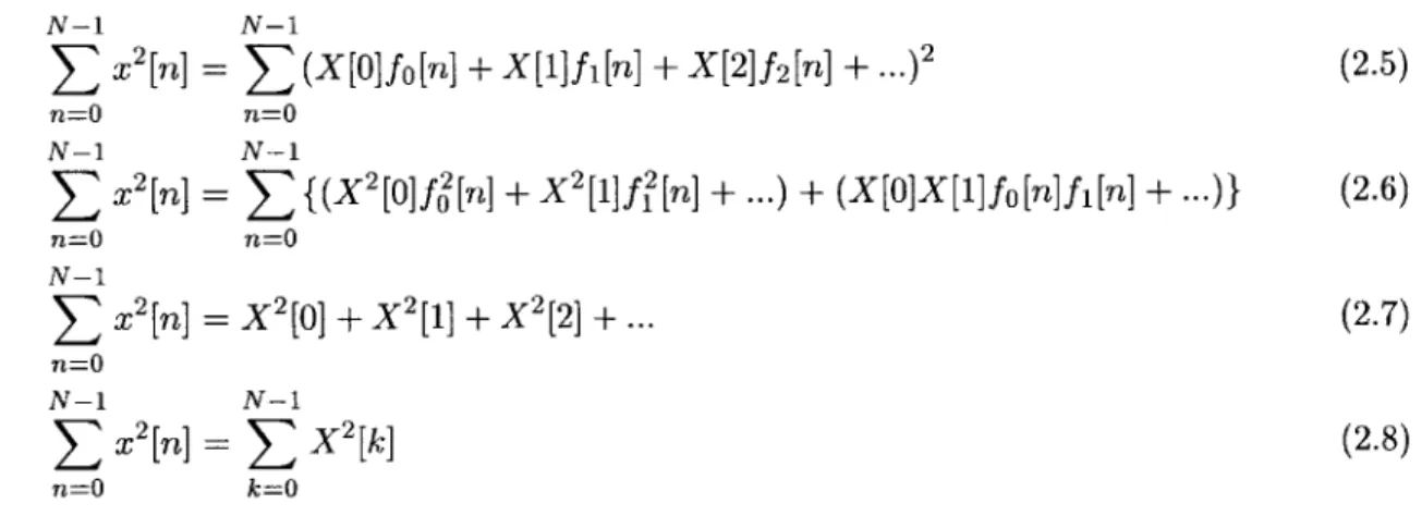
It's worth pointing out a few important properties of orthonormal transforms. The first is that the transforms are energy preserving. This is seen neatly in the following small proof.

(21)

2.1 Transformations N-I N-I

S

x2[n]

=

(X[]fo[n] + X[1]fi[n] + X[2]f

2

[n]

+n...)2

n=0 n=0 N-1 N-1

5

2[n]

=

{(X2[0]f02[n] + X

2

[1If

2[n]+ ...)

+ (X[O]X[1]fo[n]fi[n] +

...)} n=O n=O N-1 X2[n] = X2[0] + X2[1] + X2

[2]

+ n=0 N-1 N-1 X2[n]

=

X2[k] n=O k=O (2.5) (2.6) (2.7) (2.8)

A second property of orthonormal transforms follows from the above proof. The components

in the transform domain are energetically decoupled. So setting a transform coefficient X[ko] to zero removes exactly X 2 [ko] of "energy" from the signal in both the time and transform domains.

2.1.3 Vector Spaces

Exploring further the concept of orthonormal transformations, we see that these operations can be thought of as coordinate system rotations. Take for example a deterministic signal that can be represented by two points in time, say {1 1}. This signal point can be plotted on the orthonormal "time" coordinate system shown in Figure 2.2 where the x-axis and y-axis represent the trivial basis functions {1 0} and {O 1} respectively. Transforming this signal to a different orthonormal basis corresponds to rotating the axes of the "time" coordinate system. This is proven simply because of the fact that an orthonormal transform must preserve the energy of the signal. The "energy" of the signal is calculated by squaring the signal's distance from the origin, in this case 12 + 12 = 2.

1--1

-1-- S

1

Figure 2.2: Signal {1 1} A deterministic signal of length 2 represented as a point on a plane The coefficients of the transformed signal are constrained by this energy preserving property.

(22)

Thus the transform coefficients co, ci must be related by c2 + c2 = 2 This is the equation of a circle about the origin, so in this two dimensional example all that's needed to specify the orthonormal transform is a rotation angle.

Note that angle of rotation can be chosen such that all the energy is contained in one transform coefficient. Choosing the transform in this way implies that one of the basis functions is pointed exactly in the same direction as the signal of interest. In other words it is a scaled version of the signal of interest (in this case 1{1 1}). The other basis function[s] would naturally be orthogonal to the signal, (in this case {1 - 1}). Figure 2.3 shows the geometry of this example.

Figure 2.3: Transformed Signal

{V2

0} An orthonormal transformation corresponds to a

rotation of axes. In the above case, the axes are rotated so as to align with the signal point. As implied above, these concepts hold in many dimensions as well as just two. Of course it is difficult to visualize a signal of length 5 as being a point in a 5 dimensional space, save visualizing an infinite dimensional space as would be required in general for a continuous-time signal. The problem of aligning the axis in the same direction as the signal of interest can be thought of as an eigenvalue/vector problem.

2.2 Estimation of a Stochastic Signal

2.2.1 Karhunen-Loeve Transform

The example in Section 2.1 showed how a deterministic signal can be represented in two different orthonormal bases. In this thesis we are concerned with musical signals which are random in some senses and organized in others. The relation between randomness and organization can be quantified approximately by the autocorrelation function

#$2[m],

which explains how strongly correlated different sample points are with one another. Equation (2.9) defines the autocorrelation function where E{x} is the expectation of the random variable x. Note that it makes the assumption that this function is the same for all n, which is reasonable in most cases.

(23)

2.2 Estimation of a Stochastic Signal

#xx[m] = E{x[n]x[n + m]} (2.9)

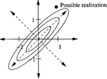
The autocorrelation function allows us to speak in probabilistic terms about random se-quences. Since we don't know a priori the energy distribution among the samples of a random process, we settle for what we do know which is the expected energy distribution among the sam-ples. We will see later that an interesting transformation is one that squeezes the most expected energy into the least number of transform coefficients. Figures 2.2 and 2.3 show this type of trans-formation where the signal is not stochastic. The same example is depicted in Figure 2.4, where the signal is stochastic and can be described by the autocorrelation matrix,

E{x[0]x[0]}

{x[0]x[1]}

]

[

#2[0]

#Xz[1

i

-

.

(2.10)

£{x[1]x[0]} E{x[1]x[1]} #'2X[-1] #5[0] . 1

Notice that the autocorrelation matrix is related only to the second-order statistics of the random process. The complete probability density functions for each random variable in the random sequence are not known. For most circumstances, this is all right, and the autocorrelation matrix proves useful. Figure 2.4 assumes that the probability density functions of each of the two samples are both Gaussian with zero mean.

Possible realization

Figure 2.4: Stochastic Signal of Length 2 A signal specified only by a mean and an autocorre-lation matrix. The ellipses are lines of constant probability.

The same transform used to rotate the coordinate system in Figure 2.3 could be used in this stochastic example to maximize the expected energy difference between x[0] and x[l]. This linear orthonormal transformation is called the Karhunen-Loeve transform and is optimal in the sense that it diagonalizes the autocorrelation matrix, and consequently places the expected energies of the transform coefficients at their maxima and minima (the eigenvalues of the autocorrelation matrix).

(24)

The basis functions are the eigenvectors of the autocorrelation matrix. So in the above example, we see that the basis functions of the KLT (Karhunen-Loeve Transform) are

{

1 -

},

and

{-2

- 9}.

More importantly the expected energies of the transform coefficients (the eigenvalues) are 1.9 and

.1. One is big and one is small.

The KLT transforms a stochastic signal into a signal with very large and very small coef-ficients. If it were necessary to approximate the signal with only a few coefficients, this property would be ideal; we needn't keep the tiny coefficients - only the big ones. We might be able to store

99% of the signal's energy in half the number of coefficients. This forms the foundation of most

compression schemes.

2.2.2 Stochastic Signal with White Noise

Consider a stochastic signal comprised of nothing but white noise. Process v[n] is white if there is no correlation between any two sample points, i.e., the autocorrelation function is given by Equation 2.11.

#,,[m] = avo6[n]

(2.11)

This corresponds to an autocorrelation matrix that is given by Equation 2.12.

&{V[0]v[0]} E{v[0]v[1]} EFfv[1]v[0]} 6fv[1]v[1]}

q$VV[0]

#vv [1]

$vv[-1] pVV[0]

The autocorrelation matrix as shown in Equation 2.12 is a multiple of the identity matrix, and therefore has eigenvalues that are always av regardless of the orthonormal transform. Geomet-rically, lines of equal probability form circles - not ellipses, so every orthonormal transform is the KLT for white noise [14].

aov 0 0 a1V

(25)

2.2 Estimation of a Stochastic Signal

2.2.3 Denoising A Stochastic Signal

This leads to the main method of denoising used in this thesis. Given a stochastic signal (music) corrupted with white noise, we seek a method of extracting the signal from the noise. The method used is similar to that used in compression. An orthonormal basis is found (preferably related to, the KL basis), and the signal is transformed to that vector space. Small coefficients are discarded, and the signal is transformed back to the time domain.

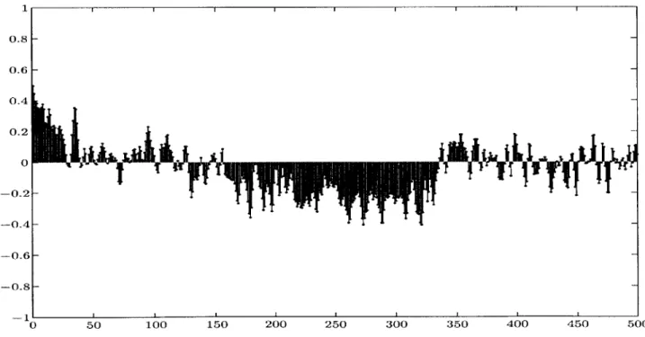
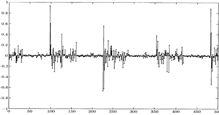
Because the transform is presumed linear, and the signal of interest is a linear sum of music x[n] and noise v[n], we expect the energy of the musical part to aggregate itself in a few coefficients (as promised by the KLT) and the distribution of energy of the noise to be unaffected by the transformation. Therefore removing small coefficients removes more noise than music (especially if the noise was small to begin with). For example if the musical part of a signal of length 1000 happened to aggregate almost all of its energy into 50 coefficients, removing the other (small) coefficients would result in removing 95% of the noise (along with a small amount of signal). The Figures below make this point graphically.

0 50 100 150 200 250 300 350 400 450

Figure 2.5: Noise Corrupted Musical Signal Represented in Time Domain

(26)

1

Figure 2.6: Noise Corrupted Musical Signal Represented in Transform Domain

l '

I I I I I I I III I

0 50 100 150 200 250 300 350 400 450

Figure 2.7: Denoised Musical Signal Represented in Transform Domain (Small cients Discarded) Here we set a threshold value and remove the smallest coefficients gaining a higher SNR

500

(27)

0 50 100 150 200 250 300 350 400 450 500

Figure 2.8: Denoised Musical Signal Represented in Time Domain The signal is recon-structed from the thresholded coefficients of Figure 2.7.

(28)

(29)

Chapter 3 Joint Time-Frequency Analysis

There are multiple ways of understanding the denoising scheme of Chapter 2. Karhunen-Loeve methods treat a musical signal like an arbitrary stochastic signal. The KL methods make the assumption that nothing except the autocorrelation matrix and the mean are known about the signal. Because of this, the KLT bears a high computational cost both in calculating the basis functions, and in actually transforming the signal [7]. Other methods are better for real-time processing.

3.1 Smooth Signals and the Time-Frequency Plane

The signals we are interested in denoising in this thesis are smooth, meaning that they are comprised of bursts of sine waves. That is the nature of music and many other natural processes. Music is made up of sequences of notes, each with harmonic content and each lasting for finite durations. Because of this information we can readily establish a basis that approximates the KL basis without enduring an undue amount of computation. The approximations are more intuitive and can prove to be more appropriate also.

The goal of the KL basis is to lump large numbers of highly correlated samples into only a few transform coefficients. Because the signals of interest are made up of small bursts of harmonically related sine waves, a good basis would be one in which one transform coefficient represented one sine wave burst.

Good bases like these are important for just the reasons outlined above. One such basis is the Short-Time Fourier Transform (STFT) [13], defined in Equation 3.1.

L-1

X[n, k] =

E x[n

+ m]w[m]ej(2

x/N)km (3.1)

(30)

The STFT is not orthonormal in general, but possesses the desirable property that the basis functions are time limited sine waves (similar to musical notes). Applying the STFT is identical to taking a spectrogram of the signal. It shows how the frequency content of the signal changes through time. The signal is transformed from the time domain to the time-frequency domain.

The time-frequency domain is a good place to operate from when denoising an audio signal. Unlike the pure frequency (Fourier) domain, there are many different transforms that could be classified as time-frequency transforms. This thesis explores the implementation of wavelet transforms, which are designed to efficiently transform from the time domain to the time-frequency domain. The wavelet transform's basis functions are little waves of finite duration, hence the name

"wavelet".

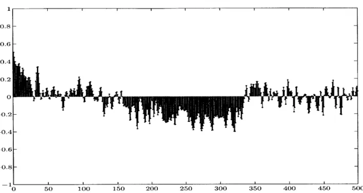
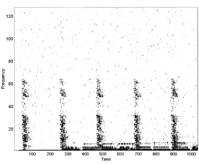
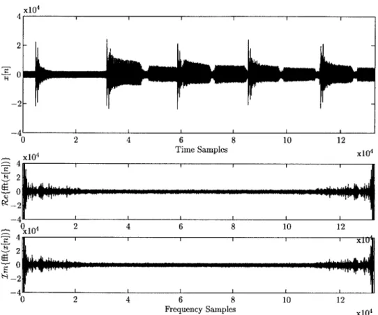
Figure 3.1 is a plot of the transform coefficients of a wavelet expansion of a piece of music corrupted by noise. The music consists of a metronome clicking each beat and a guitar playing an ascending scale. Each dot represents one transform coefficient. Because the basis functions are localized in both time and frequency, each transform coefficient occupies a region in the time-frequency plane. In the plot, we can see information about the signal that we couldn't see in either the pure time or pure frequency domains (Figure 3.2). There are many beautiful elements of wavelet transforms, and one is that orthogonality is possible. The transform used to create Figure 3.1 is orthogonal.

Notice that if we just used a low-pass filter to attempt to remove the small coefficients from the Fourier domain, we run the risk of losing the sharpness (high frequency content) of the metronome clicks. The joint time-frequency domain allows for removing selective coefficicients without disturbing the natural time-frequency structure of the music. Most of the music's energy is in the low frequency bands, but the attack of the metronome clicks are important too. Human ears hear music in both time and frequency. So the basis functions we choose should reflect a balance between what's important to the ear, and what's implementable [9]. The Karhunen-Loeve transform represents an optimal compression algorithm because it creates the best approximation of the signal with the fewest coefficients, but it might not be what the ear is looking for. This is why (although related to the KLT sometimes), working in the joint time-frequency plane is better.

3.2 Time-Frequency Transforms by Filter Banks

A way to transform a signal from the time domain to the time-frequency domain is through the use

of filter banks. The signal is put through parallel filters each of which corresponds to a different frequency band. The outputs of this type of system (shown in Figure 3.3) are multiple streams of

(31)

3.2 Time-Frequency Transforms by Filter Banks C it II 0 0 41, fi 400 500 Time 600 700 800 900 1000

Figure 3.1: Wavelet Transform Coefficients Plotted Against Time and Frequency Each coefficient can be localized in time and frequency simultaneously. The noise is spread out evenly, and much of it can be removed by setting all the light coefficients to zero.

120 100 80 >1 Ur 4) LL 60 iI i t 40 20 , I

I

quoJ

~

100 200 300

(32)

x104 4 2-0 -2--.-41 0 2 4 6 8 10 12 X104 Time Samples x10 4 4 x14 24 6 8 10 12 2 0 -2 -4 0 2 4 6 8 10 12 Frequency Samples x104

Figure 3.2: Time Waveform and Fourier Transform of the Same Signal of Figure 3.1 Although the Fourier transform does give information about the signal of interest (that it has a lot of low-frequency energy), it doesn't show the structure seen in Figure 3.1.

(33)

3.2 Time-Frequency Transforms by Filter Banks

coefficients. The STFT can be organized this way. Because the signal has been smeared through filters, each transform coefficient no longer corresponds exactly to a point in time. The coefficients correspond to regions of time, the size of which is dictated by the length of the filters in the bank.

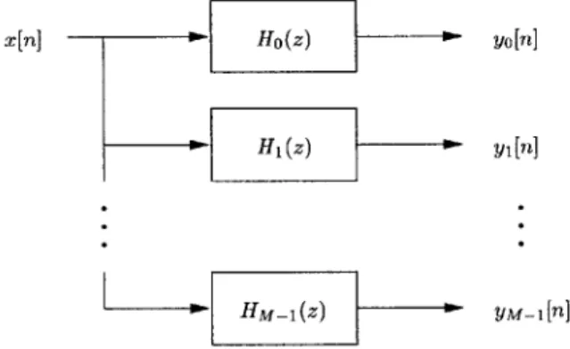
A filter bank as shown in Figure 3.3 produces M times as much data as is contained by the

signal. Most useful transforms maintain the same number of coefficients across domains, and this is guaranteed to be the case for orthogonal transforms. This is the motivation behind downsampling. In essence, the downsampling operator discards every other sample of a signal, and squeezes the remaining sample points into a sequence half its original length. Equation (3.2) defines this operator precisely.

x[n] Ho(z) yo[n]

H1(z) y1[n]

HM_1(z) yM-1[n]

Figure 3.3: General Filter Bank A signal of length N can be filtered into M frequency bands, resulting in approximately M x N output samples

y[n] = (4 2)x[n] = x[2n] (3.2)

A two-channel wavelet filter bank is shown in Figure 3.4. It is fine to discard half of the

output samples, because the filters can be designed such that any information lost in one channel is kept in the other. So if Ho(z) is low-pass, we might wish H1(z) to be high-pass. In this way each of the two transform samples occupies a different region in frequency. A transform like this cuts the time-frequency plane into 2 frequency parts, and N/2 time parts, where N is the length of the time signal.

It's extremely advantageous to maintain the same number of coefficients across the trans-form. This is because the real challenge of denoising (and taking transforms in general) lies not necessarily in the theory, but in the computation time. Faster is better. Unless needed for subtle reasons, redundant data should be discarded.

(34)

Ho2z) yo[n] x[n]

-H1(z) 2 y1[n]

Figure 3.4: Two Channel Filter Bank with Downsampling The downsampling operator

makes it possible to maintain the same number of samples in the transform domain as the time domain. No information is lost if the filters are chosen judiciously.

Using filter banks and downsampling, one can create systems of arbitrary complexity. For example, a bank like the one in Figure 3.3 can be designed with the addition of

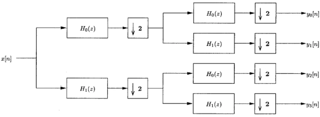
4

M operators

to eliminate hidden redundancy. Alternatively, two more two-channel banks could be put after the two outputs yo and y1 of Figure 3.4, resulting in a four-channel system. Carried further, this branching of banks results in large tree structures that turn out to have very nice computational properties. Figure 3.5 shows such a structure. Note that a structure like this also is guaranteed to be orthogonal if the intermediary two-channel banks were orthogonal.

Ho(z) 2 yo[n] Ho(z) 2 H₁(z) 2 y1[n] x[n] Ho(z) 2 y₂[n] H(z) 2 HI(z) 2 Y 3[n]

Figure 3.5: Four Channel Filter Bank Tree structures such as these prove to be computationally efficient due to the recursive nature of the tree.

The next chapter will look closely at filter banks such as the ones illustrated above. In particular we will find that systems like these can be designed to perfectly reconstruct the input given the transform. So investigating the inverses of these banks is the primary topic of Chapter 4. We will calculate the conditions for perfect reconstruction, and also see that we can create many different filter bank systems that are orthogonal or have other properties if needed.

(35)

Chapter ,

Discrete- Time Wavelets and Perfect

Reconstruction

The topic of wavelets is multifaceted. Mathematicians have their reasons for investigating them, as do engineers. This thesis is concerned with the possibility of using wavelet transforms (transforms composed of filter banks as depicted in Figure 3.4) to remove noise from a signal in real-time.

The motivation stems from the fact that the transforms are fast (comparable to the FFT) [19], and they convert from the time domain to the joint time-frequency domain which is ideal for denois-ing music and most other natural processes. The process is non-linear since it involves squelchdenois-ing coefficients to zero, not simply filtering them. The transform is non time-invariant since it involves downsampling. It might be possible to achieve close to real-time denoising in new and improved ways with wavelets.

4.1 Conditions for Perfect Reconstruction

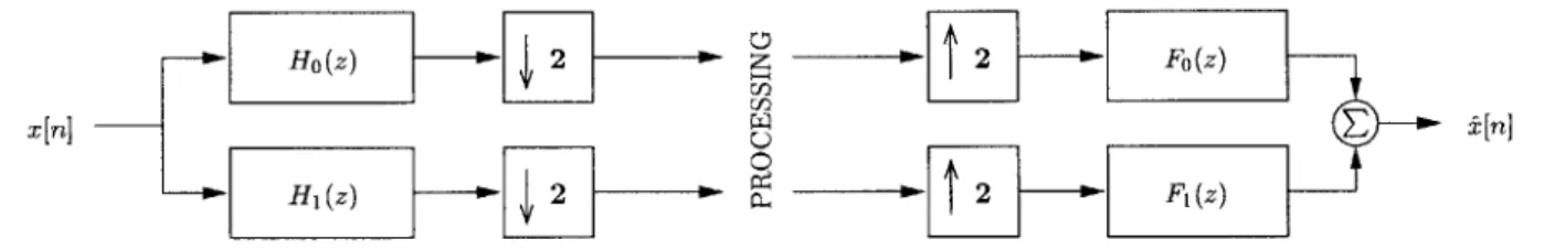
One of the advantages of working with wavelet transforms is that the analysis transform can be viewed as a filter bank. Similarly, the synthesis transform (inverse of the analysis transform) can also be represented as a filter bank. We will look first, though, at the system shown in Figure 4.1.

Ho(z)

ej2

N2 F(z)

H1(z) 2 2 F1(z)

Figure 4.1: Filter Bank Complete with Reconstruction This is a two-channel filter bank. If no processing is performed, the filters Ho(z), H1(z), Fo(z), and F1(z) can be chosen to perfectly reconstruct x[n], i.e., [n] = x[n - 1], where 1 is the delay in samples. Larger tree structures can be

built from this basic system.

(36)

z[n] = x[n - 1], where I is an overall delay. Further, it's desirable to work with causal FIR filters.

Since this thesis is concerned with near real-time processing, I should be made as small as possible. Depending on what properties of the transform are desired, a small I may or may not be possible. The system is rewritten in what's known as the polyphase form shown in Figure 4.2. Even-indexed samples are put through the first channel, and odd-Even-indexed samples through the second. Then they meet the analysis polyphase matrix, H, (z), which filters the samples appropriately.

Likewise on the synthesis side, the samples are put through the corresponding synthesis polyphase matrix, G, (z), upsampled (zeros inserted between the samples), and multiplexed. This is a useful form to work with because the conditions for perfect reconstruction (when no processing occurs) are reduced to the constraint that the product of the two polyphase matrices equal the identity. Also the polyphase form is more efficient from a computational point of view, since the downsampling is done before the filtering, saving computation.

-1 01

12

Figure 4.2: Equivalent Polyphase Form of System in Figure 4.1 The polyphase form is easier to analyze and also faster to implement since the downsampling occurs before the filtering.

Equation (4.1) shows the requirement for perfect reconstruction in terms of the polyphase matrices. It's important to recognize that an identity matrix scaled by delay z-1 _{in between}

the downsampling and upsampling will result in perfect reconstruction. If the polyphase matrices themselves were identities, the system reduces to a demultiplexer/multiplexer. It is more interesting when the two polyphase matrices are meaningful with respect to the time-frequency plane, i.e., they perform frequency filtering functions.

G,(z)H, (z) = z-'I (4.1)

Equation 4.1 can be written in expanded form,

Goo(z) _{Goi(z)] Ho(z) HOi(z)j =z-1 0,(.)}

Gio(z) Gii(z) Hio(z) HuI(z) 0 z

(37)

4.1 Conditions for Perfect Reconstruction

be impossible to achieve perfect reconstruction unless one of the two filters were IIR. This is not the case with the two channels, and it is another reason a system like this is special. Many sets of filters satisfy the perfect reconstruction constraint. It is not the goal of this thesis to analyze the pros and cons of each set. It serves as good background to mention a few things about a couple of them, however.

4.1.1 Haar and Conversion from Polyphase Form

Perhaps the simplest set of filters that satisfies PR (perfect reconstruction) is the Haar filter set. The filters in the Haar Polyphase matrix are scalars - they are zero for all n -$ 0 (4.3). They also create an orthogonal transform. All orthogonal transforms have the property that the inverse of the synthesis matrix is the conjugate transpose of the analysis matrix (G, (z) = H*T (z)). This is trivial for the Haar example.

010 (4.3)

i iJi 1 0 1

G, (z) Hp (z)

It is useful to convert the polyphase form into the more standard filter bank form shown in Figure 4.1 because it lends insight into which frequency bands the transform coefficients represent. Figure 4.3 shows the analysis filter in polyphase form. This notation is equivalent to the diagram in Figure 4.4. To understand the step from Figure 4.4 to Figure 4.6, one must use the "First Noble Identity" depicted in Figure 4.5 [19]. So Figure 4.7 finally shows the analysis bank in standard form, in terms of the polyphase filters. This relation can be summarized in (4.4). Similarly, the relation for the synthesis bank can be written as in (4.5).

2 [Hoo(z) Hoi(z)1 C [n]

x[n]

I

1

I

2 [Hio(z) Hu(z)J ci[n]

(38)

Figure 4.4: Polyphase Analysis Bank (Expanded)

x[nj M G(z) y[n]

x[n] G(zM) M y[n]

Figure 4.5: First Noble Identity in Block Diagram Form

Figure 4.6: Analysis Bank (Intermediary Form)

x[n] co[n] cl [n] x[n] co[n] c1[n]

(39)

4.1

Conditions for Perfect Reconstruction

so

Hoo (z 2) + z-'Hoi (Z2) 2 co[n]

x[n]

M- H1o(z2)+ z'HiI(z2) 2 ci[n]

Figure 4.7: Analysis Bank (Standard Form)

Ho(z) Hoo(z2) Hoi(z2)~

H1 (z) Hio(z2) H11(z2) z- 1

F0z 2 Hz)1 1

Fo(z)1 _{Foo(z2) F}₁₀_(z2)] _z-

(4.5)

F1(z) Foi(z2) Fu(z2) 1 1

With the above relations ((4.4) and (4.5)), we can create a standard filter bank given a transfer function (polyphase) matrix and its inverse. Only some analysis/inverse pairs are useful, however. The ones that are useful are usually those that produce low and high pass filters, since low and high pass filters can serve to transform into the joint time-frequency domain.

In the case of the Haar polyphase matrix, we can use relations (4.4) and (4.5) to find that the corresponding standard filters are Ho(z) = + z-1 and H1(z) = - z-1. So we see that the Haar bank does consist of a low and a high pass filter.

4.1.2 Determining Basis Functions

Just as it is meaningful to study the filters used to convert into the transform domain, it is important to know the functions that the transform coefficients represent, i.e., the basis functions. These can be calculated by eigen methods, or alternatively by simply taking impulse responses of the synthesis system. All the transforms that we have considered have been linear (perhaps not time-invariant), so the concept of linear basis functions applies.

In the case of the Haar bank in the above example, all that's needed to determine a basis function is to reconstruct a signal ,[n] from only one transform coefficient channel (co[n] = 6[n] for example). In the case of a two channel bank such as Haar, the two basis functions (one for each channel) are found by running o[n] through an upsampler and then through either Fo(z) or F1(z).

(40)

The remaining N - 2 basis functions are found similarly using 6[n - 1] in place of 6[n]. In a two

channel filter bank shown in Figure 4.1, a shift of 1 in the transform domain corresponds to a shift of 2 in the time domain. So the basis functions are composed of only two distinct shapes, repeated and shifted by two from one another.

This concept of synthesizing impulses to create basis functions proves valuable. The Haar basis function shapes are Vo(z) = + -- 1z-- and Vi(z) =- + z-1. Figure 4.8 shows the construction of basis functions by this method for a four channel system. It's interesting that every function can be represented as a sum of these four functions and their shifts by four. By this same construction the functions of Figure 4.9 are found. It is these basis functions that are referred to as the "wavelets". s s2 Fo(z) 2 -- +Fo (z) 688826---+ Fo(z) S2 - F1(z 666996-2 F- F(z)

Figure 4.8: Construction of a Single Basis Function Here we construct a basis function by passing one impulse through a reconstruction bank. Four different shapes will be produced, along with their respective shifted versions as seen in Figure 4.9

4.2 Conjugate Transpose

This section will examine the condition for orthonormality among the basis functions. Orthonor-mality imposes conditions on the polyphase matrix: it's inverse must be its conjugate transpose. Another way to arrive at the basis functions is by synthesizing impulse responses as above but in the polyphase form. This takes the form of a product of the polyphase matrix and a vector of the form {1 0 0 ...},

{0

1 0 ...}, etc. These multiplications have the effect of isolating columns of the polyphase matrix. The requirements for orthonormality, given in Chapter 2 are that the basis functions must have no correlation with one another, and they must have unity correlation with themselves.

It is just these requirements that are met by matrices that have their conjugate transpose as their inverse. This can be seen readily by multiplying such matrices by hand. Since they are

(41)

4.2 Conjugate Transpose

~~eeseese

ee 0 0eeeeeee--- e --- eee~ee --- p ~s~p p -- - - -- - - - -- - - -- - - -- --s~p - --- - - -- - -- - - - -- --- - - -- - - -- - - - -- -- ---- -- -- -- -- ---- -- ---- -- -- -- -- -- -- -- ---- -- -- -- -- -- -- -- ---- ----e e ------ - --- --------- - ---pp --p p p--

--Figure 4.9: Basis Functions of System in --Figure 4.8 Notice that there are only four distinct basis function shapes. The total number of basis functions will be equal to the length of the decomposed signal.

inverses of one another, their product is the identity,

Hoo(-z) Hio(-z) Hoo(z) Hoi(z)

1

0

Hoi(-z) Hii(-z) Hio(z) Hu1(z)J [.0 1

(4.6)

The off-diagonal zeros are formed by products like Hoo(-z)Hoi(z) + Hio(-z)H11(z) = 0.

Expanding this expression in the n domain reveals that it is the correlation function we need to to satisfy the orthogonal part of "orthonormal." The diagonal 1 terms are the normal part of

"orthonormal." This can easily be verified by hand calculation.

Orthogonality implies that inverse of the polyphase matrix must be the conjugate transpose. This means that if one matrix is causal, the other must necessarily be anti-causal. In order to circumvent this problem, we are forced to delay one of the matrices and suffer an overall delay in the system equal to 1, the length of the longest filter. This satisfies the definition of "perfect reconstruction" as stated in (4.1), but is not desirable. Later chapters will address possible solutions to this unfortunate reality, by employing non-orthogonal transforms.

(42)

(43)

Chapter 5 Near Real- Time Processing

This chapter along with the next chapters describe the original work done for this thesis. We place our attention on minimizing the delay associated with the types of transforms spoken of in earlier chapters. We seek to understand what methods of implementation will result in small delays, and what limitations different types of transforms possess.

5.1 Motivation for Real-Time

In the signal processing world, faster is always better. "Real-time" is a special case of faster because it implies that the process not only is computationally efficient, but results in an output signal that has minimal shift delay (preferably no shift delay whatsoever). This is quite an order for most systems, especially when a complex operation is desired such as denoising audio signals. In this thesis there is a tradeoff between system performance (perceived quality of processed audio) and delay.

In the audio world it is advantageous to have systems that are capable of processing in real-time. Recording engineers require the flexibility to listen to a recording with and without a given process on the fly. Moreover, an artist who wishes to perform live is only able to use equipment that can itself perform live in real-time. Noise is a central problem encountered in both recording and performing. Conventional yet sophisticated denoising apparatae that are widely used in live audio are really operating only from the time domain. They are comprised of a gate and a filter that are controlled (sometimes in clever ways) by the signal level. These systems are indeed effective, but we are interested in the possibility of increased effectiveness through transforming quickly to the time-frequency domain, and doing the gating there. Perfect reconstruction wavelet filter banks can be designed to be computationally efficient, and nearly causal which is ideal for this goal.

(44)

5.2 Measures of Performance

As to be consistent with the audio engineering literature, the primary performance measure of denoising must be perceptual [8]. Other more quantitative measures such as signal to noise ratio (SNR) are not fully representative of what sounds good to a human. When a recording has noise on it, the SNR can generally be increased by lowpass filtering the signal since most of the signal is in the lower part of the spectrum. But many have experienced the frustration of turning the treble down on a stereo system in an effort to make noisy music sound clearer. The ear is not fooled by such a trick. Certain high frequency attacks of notes (impulses) become smeared when lowpassed, and the ear realizes this and adjusts its perception. In the mind, there is still the same amount of noise present, even though the SNR has been increased.

This is the reason for transforming into the time-frequency domain. The impulses in the music can be preserved. Perhaps there is an optimal time-frequency domain with respect to which the ear perceieves the best [8]. In any case, the optimal domain to operate from should be called the "musical" domain. The musical signals themselves have been created by humans for humans. The domain that we work in should be a balance between what is found mathematically and what is known about humans and what they're expecting to hear in a clean piece of music.

Because we haven't spent a great deal of time invested in designing optimal filter banks with respect to perception (we've chosen to focus mainly on implementation issues common to all such filter bank systems), we certainly have not performed any A-B testing with human subjects. We have discovered that terrific performance is achieved when the basis functions have lengths on the order of 7000 samples in a 44.1 kHz sampled signal. This corresponds to about 0.16 seconds in time.

This figure represents a time/frequency balance where the minimal time resolution is 0.16 seconds and the maximal frequency resolution is about 70010 = 6.3 Hz. Basis functions of this length

can be achieved in two ways, assuming a system of the form shown in Figure 3.5. Long filters can be placed as Ho(z), H1(z), Fo(z), and F1(z), or more stages can be added to the tree. Both methods yield good results, although different basis functions are realized. The most important requirement for satisfactory denoising performance is that the basis functions occupy space in an appropriate time-frequency plane specified only by the length of the basis function. This length determines the approximate time/frequency balance which by far outweighs any other parameter (like basis function shape) in importance.

This is not to say that the basis function shapes are not at all important. It is implied if the basis functions have been created by a lowpass/highpass filter bank structure such as depicted

(45)

5.3 Computational Delays

in Figure 3.5 that the functions will be localized in both time and frequency. This means that the functions actually will represent a time-frequency domain. One could think of many functions that are localized in time but not in frequency such as a very high frequency oscillation added to a very slow one. A signal like this might not occupy a single localized region in frequency, but two split regions, one high and one low. So we are implicitly prioritizing that the shape of the basis functions be appropriate. This naturally happens in lowpass/highpass filter banks.

5.3 Computational Delays

As this thesis is targeted at real-time implementation, we are naturally concerned about compu-tational delays associated with the process. The group delay can be found theoretically. It is independent of system hardware, and is the delay that would occur if the hardware were infinitely fast. We have discovered that although there are limitations on this delay (particularly if we choose to work only with orthogonal filter banks), the computational delay proves to be an even harder challenge. The hardware we used progressed from a Matlab simulation to a Matlab/C hybrid language, to purely C compiled on a stand-alone Linux system.

Implementing in C is much faster than working in Matlab. But still it is not fast enough to keep up with the quickly sampled music. It is good in retrospect that this is the case, because it forced us to examine our computation methods very closely. Even though computers are becoming ever increasingly fast, the advances spur on more drive for even more sophisticated signal processing. It is naive to think that more computational power will solve signal processing problems.

Even the simplest of processes take on different forms when one tries to fully implement them. Take for instance convolution, which is represented by the * symbol. There are multitudes of methods of implementing this' [5], even though it is only a single concept in the abstract world of signals and systems. Each method has advantages and liabilities. Such is the case with our large tree structure. The next chapter, which is at the heart of the thesis, will explain our findings with respect to this implementation, and will generalize to a variety of other systems.

(46)

(47)

Chapter 6 Implementation of Wavelet Filter Bank Tree

This chapter examines the heart of the thesis: how best to implement wavelet filter bank systems with the intent of using them in near real-time. The goal of the thesis is to find a system that can be implementable in real-time, however this chapter deals primarily with finding the most efficient method of computation. This was found to be an equally, if not more important concern in the design of a system for operation in real-time.

Four different methods are considered and their associated computational costs are com-pared, using the required number of multiplies as a measure of computational efficiency. None of the methods implemented on our 200 MHz PC could keep up with the sampling rate of the music. It is natural to attempt to overcome this problem before diving heavily into designing a system with zero group delay, although the next chapter recounts our efforts to do just that in spite of significant computational delay.

The following are methods of implementing transforms like the one represented in Figure 3.5, and its associated synthesis transform.

6.1 Minimal Delay Expected

A system as in Figure 3.5 has with it a certain minimal number of time steps that are necessary

before one output sample is generated. This is what we will refer to as the minimal delay. Whereas the output of a linear filter depends on the current sample and previous samples, the transform coefficients in filter bank systems depend on the current block of M = (number of channels) samples, and past blocks. This is caused by the inclusion of the downsamplers. So for any given tree system, the minimal delay is equal to the number of channels. This delay is unavoidable, but small in comparison to other delays.

(48)

6.2 Non-Causal Approach

The most direct method is implemented by taking the whole signal and running it through each filter separately, downsampling, running the entire result through the next stage of filters, and so on. This is clearly not an option for us since it requires the entire signal in advance. It is non-causal, but might work theoretically for signals that are to be post-processed, such as previously recorded music. Even if we had access to the whole signal before processing, this idea has the same major pitfalls that convolving enormous signals has. Unless the signal of interest is short, it is unwieldy to work with in this way, due to memory constraints.

It is important to study the number of multiplications that are associated with this direct method, however, because it lends insight into the cost or benefit of computing the same result in another fashion. We did not actually implement this system for the reasons stated above (memory), but the number of multiplications can nevertheless be computed.

The specific transform that was studied in this thesis is a 128 channel filter tree with length

30 filters. Assuming an input signal of 10, 000 samples, we can calculate the number multiplications

this direct method would require.

A convolution operation between two signals, of lengths m and n, requires m x n

multipli-cations. Convolution followed by downsampling can be produced in " multiplications, since it is not necessary to calculate the samples that will be discarded. The length of a convolved signal becomes m + n - 1. A signal of length n becomes a signal of length ' or if odd n-1 after down-sampling. Also, upsampling a signal of length n results in a signal of length 2n - 1. Upsampling

followed by filtering requires )m "2 multiplications. From these facts, we can derive the number of multiplications required for all of our implementations.

The number of multiplications that the direct method requires can be found by constructing Table 6.1. Similarly, on the synthesis side, we can calculate the number of multiplies that would be required by constructing Table 6.2. The total number of multiplies associated with this process is the sum of the two totals: 421, 438, 980. As a rule of thumb, the number of multiplies for a system like this, assuming a long input signal relative to the length of the filters 1, and number of stages